Abstract

The efficient numerical solution of Non-LTE multilevel transfer problems requires the combination of highly convergent iterative schemes with fast and accurate formal solution methods of the radiative transfer (RT) equation. This contribution begins presenting a method for the formal solution of the RT equation in three-dimensional (3D) media with horizontal periodic boundary conditions. This formal solver is suitable for both, unpolarized and polarized 3D radiative transfer and it can be easily combined with the iterative schemes for solving non-LTE multilevel transfer problems that we have developed over the last few years. We demonstrate this by showing some schematic 3D multilevel calculations that illustrate the physical effects of horizontal radiative transfer. These Non-LTE calculations have been carried out with our code MUGA 3D, a 3D multilevel Non-LTE code based on the Gauss-Seidel iterative scheme that Trujillo Bueno and Fabiani Bendicho (1995) developed for RT applications.

1 Introduction

To what extent can we trust diagnostic results obtained with the assumption that the solar atmospheric plasma is composed of homogeneous plane-parallel layers or via approximations that neglect horizontal radiative transfer (RT) effects? How important are the errors in the magnetic fields, temperatures and velocities inferred by confronting spectro-polarimetric observations with Non-LTE 1D RT model calculations? Clearly, to provide proper answers to questions like these requires to develop first efficient 3D RT methods that allow Non-LTE effects in complex atomic models with many levels and transitions to be rigorously investigated.

There is a second reason which makes the development of fast iterative methods for 3D Non-LTE RT so relevant. This is because processes of energy exchange by radiation play an important role in the structure and dynamical behaviour of the stellar magnetized plasma. Thus, for instance, if one wishes to perform time-dependent radiation hydrodynamics simulations similar to those carried out by Carlsson and Stein (1997), but in 3D instead of 1D, it turns out to be imperative to have first access to numerical methods capable of accurately yielding the self-consistent atomic level populations at the cost of only very few formal solution times.

The efficient solution of multilevel transfer problems requires the combination of a highly convergent iterative scheme with a fast formal solver of the RT equation. In Section 2 we briefly comment on a hierarchy of iterative schemes that can be applied for solving multilevel Non-LTE problems with increasing improvements in the convergence rate and total computational work. The 3D multilevel transfer calculations that we present in this contribution have been obtained by combining a highly convergent iterative scheme based on Gauss-Seidel iteration (Trujillo Bueno and Fabiani Bendicho, 1995) with a fast 3D formal solver that has parabolic accuracy (see Section 3). As was the case with our 2D formal solver, our generalization to 3D is based on the “short-characteristics” method of Kunasz and Auer (1988). Our 3D multilevel code is called MUGA 3D (“Multi-level Gauss-Seidel Method”) and it is substantially faster than our code MALI 3D, which is based on Jacobi iteration (see Rybicki and Hummer, 1991; Auer, Fabiani Bendicho and Trujillo Bueno, 1994).

Section 3 briefly describes our 3D formal solver as applied to the scalar transfer equation for the specific intensity (I). In order to be able to consider 3D atmospheric models where solar plasma structures repeat themselves along the horizontal directions we choose horizontal periodic boundary conditions along the Cartesian coordinates X and Y. Although we do not give any details here, we have also generalized to 3D the Stokes-vector 1D formal solver method developed by Trujillo Bueno (1998), which is based on the matrix exponential approximation to the evolution operator.

In Section 4 we show some illustrative 3D multilevel transfer calculations for a 5-level Ca II model atom where the H, K and infrared triplet lines are treated simultaneously, taking fully into account the interlockings by which photons are converted back and forth between the different line transitions in the assumed 3D medium. Here we consider schematic 3D solar models characterized by horizontal sinusoidal temperature inhomogeneities. With the help of these 3D multilevel calculations we are able to illustrate some subtle effects of horizontal radiative transfer that are important for the correct interpretation of high spatial resolution observations. Finally, Section 5 gives our conclusions.

2 Iterative Methods for Multilevel Transfer

The simplest procedure one might think of to solve self-consistently the kinetic and RT equations is $\Lambda-$iteration: using the current estimate of the atomic level populations at each spatial grid-point (or, more in general, of the irreducible tensor components of the atomic density matrix; see Trujillo Bueno 1999) evaluate the absorption and emission coefficients. Next, solve the radiative transfer equation and compute the radiation field intensity in all transitions. Finally, with the radiative rates obtained, solve the kinetic equations at each spatial grid-point independently and obtain a new estimate of the atomic level populations. However, as is well known, under typical NLTE conditions in optically thick media this $\Lambda-$ iteration method converges extremely slowly. This is certainly regrettable because with this method there is no need of inverting large matrices and the computing time per iteration is minimal. In any case, as demonstrated by Trujillo Bueno and Manso Sainz (1999), in solar-like atmospheres the $\Lambda-$ iteration method can be used to find the self-consistent solution of Non-LTE polarization transfer problems if one initializes using the “exact” solution corresponding to the unpolarized transfer case.

The dream of numerical RT is to develop iterative methods where everything goes as simply as with the $\Lambda-$iteration scheme, but for which the convergence rate is extremely high. The iterative methods for RT applications based on Gauss-Seidel iteration that we have developed over the last few years have been worked out with this motivation in mind. Their convergence rate is extremely high, there is no need of constructing and inverting any large matrix, and the computing time per iteration is similar to that of the $\Lambda-$iteration method. A full account of these developments can be found in the following publications:

1) Auer, Fabiani Bendicho and Trujillo Bueno (1994) present the generalization of the Jacobi-based MALI method of Rybicki & Hummer (1991) to multilevel RT in 2D. They also developed a short-characteristics strategy to do the formal solution in 2D Cartesian coordinates with horizontal periodic boundary conditions. Of particular interest is a simple grid-doubling technique which both rapidly finds the converged solution in fine meshes and automatically estimates its corresponding true error. The total computational work scales as ${\rm NP}^{2}$, with NP the total number of spatial grid-points in a fixed computational domain.

2) Trujillo Bueno and Fabiani Bendicho (1995) developed a novel iterative scheme based on Gauss-Seidel (GS) iteration (MUGA). This is the paper on which our present work is based on. The total computational work scales as ${\rm NP}^{2}/4$ for the pure GS method (implemented as suggested in the conclusions of their paper), and as ${\rm NP}{\sqrt{\rm NP}}$ for the successive overrelaxation (SOR) method. This paper was fundamental for a successful development of our non-linear multigrid method for RT applications.

3) Fabiani Bendicho, Trujillo Bueno and Auer (1997) consider the application of the non-linear multigrid method (see Hackbush, 1985) to multilevel RT. Here the iterative scheme is composed of two parts: a smoothing one where a small number of MUGA iterations on the desired finest grid are used to get rid of the high-frequency spatial components of the error in the current estimate, and a correction obtained from the solution of an error equation in a coarser grid. With this method the total computational work scales simply as NP, although it must be said that the computing time per iteration is about 4 times larger than that required by the $\Lambda-$iteration method.

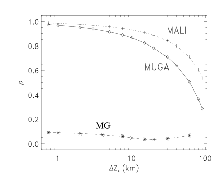
Figure 1.  : Variation with the grid-spacing $\Delta{z}$ of the maximum eigenvalue of the iteration operator corresponding to several multilevel iterative schemes. The MG symbol refers to our non-linear multigrid code.

In order to compare the convergence rates of these three iterative methods, we present in Fig. 1 an estimate of the maximum eigenvalues ($\rho$) of the corresponding iteration operator, which controls the convergence properties of such iterative schemes (see Trujillo Bueno and Fabiani Bendicho, 1995). The knowledge of this maximum eigenvalue ($\rho$) is useful because errors decrease as ${\rho}^{itr}$, where “$itr$” is the iterative step. We obtain this information from multilevel Ca II calculations in several 1D grids with decreasing grid-size ($\Delta{z}$) by calculating $R_{c}(itr+1)/R_{c}(itr)$ for $itr>>1$, where $R_{c}(itr)$ is the maximum relative change in the level populations. As it can be noted in Fig. 1 the convergence rate of both, the MALI and MUGA schemes decreases when the spatial resolution of the grid is improved, while the maximum eigenvalue of our non-linear multigrid method is always very small ($\rho\sim 0.1$) and insensitive to the grid-size. A maximum eigenvalue $\rho=0.1$ means that the error decreases by one order of magnitude each time we perform an iteration. This explains that, typically, two multigrid iterations are sufficient to reach the self-consistent solution for the atomic level populations.

The 3D multilevel calculations shown in this contribution were obtained with our code MUGA 3D, i.e. with a multilevel GS scheme based on the paper by Trujillo Bueno and Fabiani Bendicho (1995) combined with the following 3D formal solver. In practical applications we always use MUGA 3D with Ng (1974) acceleration.

3 The 3D formal solver.

The scalar RT equation for the specific intensity is

$${{{\rm d}{\rm I}_{\nu}}\over{{\rm d}{s}}}\,=\,{\chi_{\nu}}\,(\,{\rm S}_{\nu}\,-\,{\rm I}_{\nu}\,)\,,$$ (1)

where $s$ is the geometric distance along the ray propagating in a certain direction in a 3D medium, $\chi_{\nu}$ is the total opacity and ${\rm S}_{\nu}$ the source function.

Figure 2.  : 3D Cartesian spatial grid surrounding the grid-point of interest (O) where the specific intensity ${\rm I}_{\rm O}$ is to be calculated. This is done by solving analytically the integral of Eq. (2) along the short-characteristics MO corresponding to the ray of direction $\vec{\Omega}$.

We now consider a 3D Cartesian spatial grid (see Fig. 2). Point O is the grid-point of interest at which one wishes to calculate the specific intensity ${\rm I}_{\rm O}$, for a given frequency ($\nu$) and a direction (${\vec{\Omega}}$). Point M is the the intersection point with the grid-plane that one finds when moving along $-\vec{\Omega}$. At this upwind point we assume that the specific intensity ${\rm I}_{\rm M}$ for the same frequency and angle is known from previous steps. In a similar way, point P is the intersection point with the grid-plane that one encounters when moving along $\vec{\Omega}$. We also introduce the optical depths along the ray between points M and O ($\Delta{\tau}_{\rm M}$) and between points O and P ($\Delta{\tau}_{\rm P}$). From the formal solution of the previous transfer equation one finds that

$${\rm I}_{\rm O}={\rm I}_{\rm M}\,{\rm e}^{-\,\Delta{\tau}_{\rm M}}\,+\,\int_{0}^{\Delta{\tau}_{\rm M}}\,{\rm S}(t){\rm e}^{-({\Delta{\tau}_{\rm M}}\,-\,t)}\,dt,$$ (2)

where the optical depth variable $t$ is measured from M to O.

The integral of Eq. (2) can be solved analytically by integrating along the short-characteristics MO assuming some prescribed variations for the source function (e.g. linear variation along M and O, or parabolic along M,O and P, or cubic-centered around point O, etc.). Our 3D formal solution method assumes that the source function ${\rm S}(t)$ varies parabolically along M,O and P. The result reads:

$${\rm I}_{\rm O}={\rm I}_{\rm M}\,{\rm e}^{-\Delta{\tau}_{\rm M}}\,+\,{\Psi}_{\rm M}{\rm S}_{\rm M}\,+\,{\Psi}_{\rm O}{\rm S}_{\rm O}\,+\,{\Psi}_{\rm P}{\rm S}_{\rm P},$$ (3)

where $\Psi_{\rm X}$ (with X either M, O or P) are given in terms of the quantities $\Delta{\tau}_{\rm M}$ and $\Delta{\tau}_{\rm P}$ that we evaluate numerically by assuming that ${\rm ln}(\chi)$ varies linearly with the geometrical depth, $\chi$ being the opacity.

It is very important to point out that one should avoid the use of a formal solution method based on a linear interpolation formula, i.e. one should avoid assuming that, for each grid-point O of interest, the source function varies linearly along points M and O. Otherwise, the accuracy of the self-consistent solution will never be better than about 10$\%$, even by choosing a very large number of grid-points per opacity scale height (see Trujillo Bueno, 1998). The reason for this is that the use of linear interpolation for ${\rm S}(t)$ leads to formal solution methods that are unable to yield the correct asymptotic behaviour for the intensity when having nonlinear source functions in optically thick atmospheres. We emphasize that our 3D formal solution method is based on the above-mentioned parabolic approximation and it only uses the linear approximation formula for calculating the radiation field at the upper and lower boundaries for rays going out of such boundaries. However, as we illustrate below, the use of the parabolic approximation for investigating problems where we have sudden variations in the physical quantities requires to implement it using an improved version of the monotonic upwind interpolation technique applied by Auer and Paletou (1994).

The application of this formal solution method in 1D is straightforward. A detailed description of how to implement it in 2D slabs with prescribed irradiation on the lateral boundaries can be found in Kunasz and Auer (1988) and Auer and Paletou (1994). In 2D with horizontal periodic boundary conditions is slightly more complicated and a suitable strategy has been described by Auer, Fabiani Bendicho and Trujillo Bueno (1994).

The main changes when going to 3D imposing horizontal periodic boundary conditions lie in the interpolation. We have assumed that $\rm I_{M}$ is known (see Fig. 2) but, in most cases, the M-point (like the point P) will not be a grid-point of the chosen 3D spatial grid. The intensity at this M-point has to be calculated by interpolating from the available information at the nine surrounding grid-points, as we must also do for obtaining the opacities and source functions at M and P.

Parabolic interpolation can however generate spurious negative intensities if the spatial variation of the physical quantities is not well resolved by the spatial grid. This happens, for instance, if one tries to simulate the propagation of a beam in vacuum using a three dimensional grid. The analytical solution in this case is simply $\rm I_{O}=I_{M}$, and any numerical error is due to the effect of the conventional way of applying the parabolic interpolation. To avoid these problems we have improved the 1D monotonic interpolation strategy of Auer and Paletou (1994), and generalized it to the two-dimensional parabolic interpolation that is required for 3D RT calculations (Fabiani Bendicho and Trujillo Bueno, in preparation).

Figure 3.  : Ray propagating in vacuum. Emergent intensity with parabolic interpolation implemented without (a) and with (b) our improved version of the monotonic upwind interpolation strategy.

In Fig. 3 we show the intensity that emerges from a 3D computational box after having illuminated its lower boundary with a beam of given intensity. Here the aim is to simulate a beam propagating in vacuum. Using standard parabolic interpolation (Fig. 3a) leads to unphysical negative intensities. However, with our improved version of the upwind monotonic interpolation strategy we guarantee that the parabolic interpolation is not introducing spurious sources and sinks and its second order accuracy is maintained.

For solving Non-LTE radiative transfer problems as shown above the chosen formal solution method has to be implemented in a way such that it rapidly computes, at each spatial grid-point, the radiation field for each frequency and direction of the chosen numerical quadratures together with the diagonal element of the $\Lambda-$operator. To this end, one may also try with higher-order methods if desired. We have found that our parabolic formal solvers are fast and accurate enough, stable and easy to work with independently of the geometry and of the iterative method used.

4 Illustrative 3D multilevel results

Our aim here is to study a few illustrative results for Ca II in a schematic 3D atmospheric model characterized by the following temperature structure:

$$\rm T(X,Y,Z)\,=\,5000\,+\,500\,sin(a\,X)\,\,sin(b\,Y),$$ (4)

where $\rm a=2\pi/P_{x}$ and $\rm b=2\pi/P_{y}$, with ${\rm P}_{x}$ and $\rm P_{y}$ the horizontal periods along the X and Y Cartesian coordinates, respectively. For this example we choose $\rm P_{x}\,=\,P_{y}\,=1000$ km. We also assume that the total hydrogen number density is exponentially stratified along the vertical direction (Z) with a scale height $\cal H$=100 km. We adopt a standard 5-level Ca II atomic model and a constant electron density $n_{e}=10^{11}\,{\rm cm}^{-3}$. We compare our full 3D multilevel results with the corresponding 2D multilevel calculation and with results obtained using a well-known approximation that neglects the effect of horizontal RT on the level populations, i.e. with the so-called $1.5{\rm D}$ approximation (Mihalas, Auer and Mihalas, 1978; Solanki, Steiner and Uitenbroek, 1991).

We point out that our calculations do take into account the change in the line opacities caused by the assumed 500 K horizontal temperature inhomogeneities. Thus, the 3D multilevel transfer effects are the result of the combined action of the smoothing effect of the source-function fluctuations (Spiegel, 1957; Kneer and Trujillo Bueno, 1987) and the channelling effect due to the opacity fluctuations (Cannon, 1970; Trujillo Bueno and Kneer, 1990). Since we use a 5-level atomic model, we can examine the 3D effects for the H, K and the infrared triplet lines. Figures 4, 5 and 6 give the variation with X and Y of the vertically emergent intensity at the continuum frequency (upper part) and at the line core (lower part). We only show this for the H and 8662 ${\rm\AA}$ lines since for the K line and the other two infrared lines very similar results were found.

Figure 4.  : The vertically emergent intensity at the line core (lower surface plot) and at the continuum frequency (higher surface plot) corresponding to the $1.5{\rm D}$ approximation applied to a model atmosphere with ${\rm P_{x}=P_{y}}=1000$ km. These intensities are shown for the H and 8662 ${\rm\AA}$ Ca II lines in the left and right panels of the figure, respectively. Geometrical distances are measured in units of the opacity scale height $\cal H$.

Fig. 4 corresponds to calculations carried out with the $1.5{\rm D}$ approximation. As pointed out above this approximation completely neglects the effects of horizontal RT on the level populations. Consequently, the result is that, not only at the continuum frequency, but also at the line center the emergent intensity shows large horizontal fluctuations. The $1.5{\rm D}$ atomic level populations have large horizontal fluctuations at all atmospheric depths, simply because one is here neglecting the smoothing and channelling horizontal 3D RT effects when solving the kinetic and RT equations.

Figure 5.  : 2D vertically emergent intensities. For more information see Fig. 4.

Fig. 5 shows the 2D multilevel transfer results (see also Auer, Fabiani Bendicho and Trujillo Bueno, 1994). Here it was assumed that the model’s temperature was only fluctuating along the horizontal X-direction with $\rm P_{x}=1000$ km; i.e. horizontal transfer effects along the Y-direction are completely neglected. The explanation of the results is the following: above the height of thermalization, 2D horizontal transfer effects are efficiently damping the horizontal fluctuations of the populations of the two uppermost levels of the chosen 5-level Ca II model atom. This smoothing is translated to the line source functions, which are proportional to $n_{4}A_{4,1}$ for the H line and to $n_{4}A_{4,2}$ for the 8662 ${\rm\AA}$ line, with $A$ the Einstein coefficient for spontaneous emission. Thus, since the continuum photons come from the deepest layers, one sees strong horizontal intensity fluctuations at continuum frequencies, while at the line core one finds horizontal intensity fluctuations of very small amplitude because these photons come from the higher atmospheric layers. Note that, both for the H and the 8662 ${\rm\AA}$ infrared lines, the vertically emergent intensities are fluctuating in phase with the assumed thermal inhomogeneities.

Figure 6.  : 3D vertically emergent intensities. For more information see Fig. 4.

Fig. 6 depicts the results of our full 3D multilevel calculation with $\rm P_{x}\,=\,P_{y}=1000$ km. For the H line the result is qualitatively similar to the 2D results, although the amplitude of the horizontal intensity fluctuations at line-center is significantly smaller, as expected from the fact that in 3D the horizontal transfer effects are enhanced with respect to those found for the 2D case. However, for the 8662 ${\rm\AA}$ line we find a result that, at first sight, might appear surprising: at line center the resulting horizontal fluctuation of the vertically emergent intensities is anticorrelated with respect to the fluctuation of the assumed thermal inhomogeneities. In other words, at the line core of this infrared line, one gets more intensity from the coolest atmospheric points than from the hottest ones. The explanation is that the IR line source function shows a change, by $\pi$, in phase above the height ($h_{c}$) in the atmosphere where the amplitude of the horizontal fluctuation in $n_{4}$ is greatly diminished. And this change of phase is, in turn, due to the fact that the line source function is the result of dividing an almost non-fluctuating emissivity by a line opacity (essentially set by $n_{2}$) that fluctuates in phase with the assumed temperature inhomogeneities. This occurs both in 2D and in 3D, but with the difference that $h_{c}^{2D}\,>\,h_{c}^{3D}$ for given values of $\rm P_{x}$ and $\rm P_{y}$. In fact, one finds indeed a similar result in 2D, but for $\rm P_{x}$ values significantly smaller than 1000 km. Since the horizontal transfer effects are more important in 3D than in 2D, it turns out that such an effect already sets in at $\rm P_{x}=P_{y}=1000$ km.

We thus see that our 3D multilevel calculations demonstrate the efficiency of horizontal RT effects and confirm (see Kneer, 1981; Trujillo Bueno, 1990) that the interpretation of high-spatial resolution observations ignoring the existence of horizontal transfer effects (as is done when using the $1.5{\rm D}$ approximation) may substantially underestimate the actual inhomoheneities present in the solar atmospheric plasma.

5 Concluding Remarks

We have developed a 3D multilevel code (MUGA-3D) that combines the Gauss-Seidel iterative scheme of Trujillo Bueno and Fabiani Bendicho (1995) with a 3D formal solver that uses horizontal periodic boundary conditions. With this new code we have performed some 3D multilevel simulations that highlight the importance of carefully investigating the effects of horizontal radiative transfer using realistic atmospheric and atomic models.

We point out that our 3D formal solver can be used not only for solving “unpolarized” multilevel transfer problems, but also resonance line polarization and Hanle effect problems, like those considered in these Proceedings by Manso Sainz and Trujillo Bueno (1999), Paletou et. al. (1999) or Dittmann (1999). This is because, for these polarization transfer cases, the absorption matrix is diagonal. As a result, we have similar equations for the Stokes I, Q and U parameters.

However, for the solution of more general polarization transfer problems, like the Non-LTE Zeeman line transfer case considered by Trujillo Bueno and Landi Degl’Innocenti (1996), but in 3D instead of 1D, one needs a 3D formal solution method of the Stokes-vector transfer equation. This is because here the absorption matrix turns out to be a full $4\times 4$ matrix and all the Stokes parameters are coupled together. To this end we have generalized to 3D the Stokes-vector formal solver developed by Trujillo Bueno (1998), which can be considered as a generalization to polarization transfer of the short-characteristics method.

We would like to end this paper by saying that over the last 10 years we have witnessed impressive progress concerning the development of highly convergent iterative schemes and accurate formal solvers for RT applications. Now it is time to apply them with physical intuition in order to improve our knowledge of the Sun, its magnetic field and its polarized spectrum.