Exact analytical solution of the problem of current-carrying states of the Josephson junction in external magnetic fields

Abstract

The classical problem of the Josephson junction of arbitrary length $W$ in the presence of externally applied magnetic fields ($H$) and transport currents ($J$) is reconsidered from the point of view of stability theory. In particular, we derive the complete infinite set of exact analytical solutions for the phase difference that describe the current-carrying states of the junction with arbitrary $W$ and an arbitrary mode of the injection of $J$. These solutions are parameterized by two natural parameters: the constants of integration. The boundaries of their stability regions in the parametric plane are determined by a corresponding infinite set of exact functional equations. Being mapped to the physical plane $\left(H,J\right)$, these boundaries yield the dependence of the critical transport current $J_{c}$ on $H$. Contrary to a wide-spread belief, the exact analytical dependence $J_{c}=J_{c}\left(H\right)$ proves to be multivalued even for arbitrarily small $W$. What is more, the exact solution reveals the existence of unquantized Josephson vortices carrying fractional flux and located near one of the junction edges, provided that $J$ is sufficiently close to $J_{c}$ for certain finite values of $H$. This conclusion (as well as other exact analytical results) is illustrated by a graphical analysis of typical cases.

I Introduction

Based on mathematical methods of stability theory, we reconsider the classical physical problemS72 ; BP82 ; L86 of current-carrying states of the Josephson junction of arbitrary length $W$ in external magnetic fields. Although the problem was first posed over four decades agoJ65 ; ISS66 ; OS67 and ever since has found numerous practical applications,S72 ; BP82 ; L86 ; r1 its complete analytical solution has not been obtained in the previous literature. Here, we derive this solution and show that it leads to new and important physical conclusions: the multivaluedness of the exact analytical dependence of the critical transport current on the applied field for arbitrarily small $W$, and the existence of unquantized Josephson vortices carrying fractional flux. This paper can be considered as a logical continuation of the investigation initiated in our preceding publication,KG06 where we have derived the complete analytical solution for the Josephson junction in external magnetic fields in the absence of transport currents.

To remind the reader of the standard formulation of the problem, we consider the geometry presented in Fig. 1. Here, the $x$ axis is perpendicular to the insulating layer $I$ (the barrier) between two identical superconductors $S$; the $y$ axis is along the barrier whose length is $W=2L\in\left(0,\infty\right)$. A constant, homogeneous external magnetic field $\mathbf{H}$ is applied along the axis $z$: $\mathbf{H}=\left(0,0,H\geq 0\right)$. Full homogeneity along the $z$ axis is assumed. The transport current $\mathbf{J}$ is injected along the axis $x$: $\mathbf{J}=\left(J,0,0\right).$

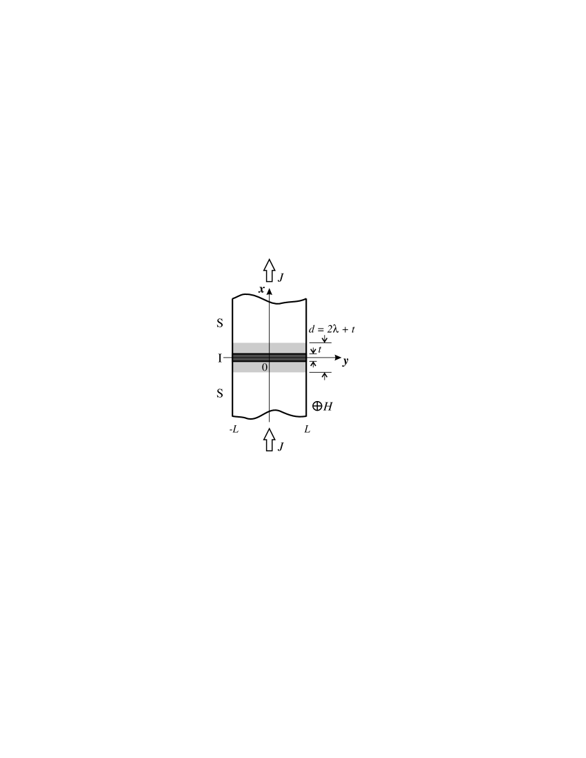
Figure 1: The geometry of the problem: $t$ is the thickness of the barrier; $W=2L$ is the length of the barrier; $\lambda$ is the London penetration depth; $d=2\lambda+t$ is the width of the field-penetration region (shaded). The external magnetic field $H$ is directed into the plane of the figure, and the transport current $J$ is along the axis $x$.

In the region of field penetration, the electrodynamics of the junction in equilibrium is fully described by a time-independent phase difference at the barrier, $\phi=\phi\left(y\right)$. Using the dimensionless units introduced in Ref. KG06 , we can write down the local magnetic field and the Josephson current density asJ65

$$h\left(y\right)=\frac{1}{2}\frac{d\phi}{dy}$$ (1)

and

$$j\left(y\right)=\frac{1}{2}\sin\phi\text{,}$$ (2)

respectively. Accordingly, the equation for the phase difference (the Maxwell equation) reads:

$$\frac{d^{2}\phi}{dy^{2}}=\sin\phi.$$ (3)

Boundary conditions to (3) depend on the mode of the injection of the transport current

$$J=\int_{-L}^{L}dyj\left(y\right).$$

If it is symmetric with respect to the plane $\left(y,z\right)$, we have:

$$\frac{d\phi}{dy}\left(\pm L\right)=2H\pm J,$$ (4)

or, equivalently,ISS66 ; OS67

$$H=\frac{1}{4}\left[\frac{d\phi}{dy}\left(+L\right)+\frac{d\phi}{dy}\left(-L\right)\right],$$ (5)

$$J=\frac{1}{2}\left[\frac{d\phi}{dy}\left(+L\right)-\frac{d\phi}{dy}\left(-L\right)\right].$$ (6)

Solutions to (3), (4) are supposed to satisfy an obvious physical requirement: they must be stable with respect to any infinitesimal perturbations. (Unstable solutions that do not meet this requirement are physically unobservable and should be rejected.)

Unfortunately, the standard boundary-value problem (3), (4) is mathematically ill-posed:CH (i) for $\left|J\right|$ larger than certain $J_{\max}=J_{\max}\left(H,L\right)$, it does not admit any solutions at all; (ii) aside from stable (physical) solutions, there may exist unstable (unphysical) solutions for the same $H$ and $J$; (iii) for the same $H$ and $J$, there may exist several different physical solutions. An immediate consequence of this ill-posedness is as follows: although the general solution to (3) is well-known,A70 the constants of integration specifying particular physical solutions cannot be determined directly from the boundary conditions (4).

In view of the above-mentioned mathematical difficulties, the previous analysis of the problem (3), (4) was concentrated mainly on finding the dependence $J_{\max}=J_{\max}\left(H\right)$ (for particular values of $L$) without trying to establish the exact analytical form of current-carrying solutions. (It should be noted that the quantity $J_{\max}$ itself was identified with the experimentally observable critical current $J_{c}$, i.e., the identity $J_{\max}\equiv J_{c}$ was assumed.)

For the case $L\ll 1$, there existedJ65 a simple analytical approximation for the dependence $J_{\max}=J_{\max}\left(H\right)$ (the so-calledS72 ; BP82 ; L86 ”Fraunhofer pattern”). As to the case $L\gtrsim 1$, only particular numerical results were obtained. Thus, Owen and ScalapinoOS67 established the dependence $J_{\max}=J_{\max}\left(H\right)$ only for $L=5$: it proved to be multivalued. The numerical method of Ref. OS67 was later employed to study the effect of asymmetric injection of the transport current.BB75 Unfortunately, all these numerical results could tell very little about general properties of the current-carrying states for arbitrary $L\in\left(0,\infty\right)$. Besides, no analytical expressions were derived that could serve for direct determination of $J_{\max}$.

On the other hand, attempts were madeZh78 ; ZhZ78 to simplify the computational procedureOS67 by transforming the boundary-value problem (3), (4) into an equivalent initial-value problem. Although these attempts did not produce exact analytical solutions, we note that Refs. Zh78 ; ZhZ78 introduced a new, more satisfactory mathematical definition of the observable critical current $J_{c}$: it was identified with the boundary of the stability regions of the current-carrying configurations. The same mathematical definition of $J_{c}$ was employed in Refs. Ga84 ; Se04 concerned with certain nontrivial generalizations of the boundary-value problem (3), (4). Unfortunately, exact analytical expressions for the physical solutions to (3), (4) were not found in Refs. Ga84 ; Se04 , either.

As already mentioned, in Ref. KG06 we have derived the complete infinite set of exact physical solutions to (3), (4) under the condition $J=0$. The approach of Ref. KG06 consists in a certain generalization of the boundary conditions and an application of methods of stability theory at an early stage of the consideration. The same approach is adopted in this paper for the general case $J\neq 0$. Thus, we derive a complete set of exact particular solutions to (3) that are stable under the condition that $\frac{d\phi}{dy}$ is fixed at the boundaries $y=\pm L$ [for arbitrary $L\in\left(0,\infty\right)$]. These solutions are parameterized by two natural parameters: the constants of integration of (3). The boundaries of their stability regions are determined by a corresponding infinite set of exact functional equations. The physical interpretation of the obtained solutions stems from the fact that the boundary conditions in the form (5), (6) (or their modification for the case of asymmetric injection of $J$) realize a mapping of the stability regions from the parametric plane to the physical plane $\left(H,J\right)$.

In Sec. II, we present a static method of the analysis of stability based on the minimization of the generating free-energy functional. A Sturm-Liouville eigenvalue problem that plays a key role in the analysis of stability is discussed. In Sec. III, we derive the complete set of exact stable analytical solutions to (3), (4) under the condition $H\geq 0$, $J\geq 0$. A numerical analysis of several typical cases is carried out. In Sec. IV, we elaborate on major physical implications of the exact analytical solutions. Graphic illustrations are presented. Generalizations to the case of arbitrary sign of $H$ and $J$, and to the case of asymmetric injection of $J$ are considered. Finally, in Sec. V, we summarize the obtained physical and mathematical results and make several concluding remarks.

In Appendix A, an alternative (dynamic) method of the analysis of stability is presented. In Appendix B, functional equations for the stability regions are derived. In Appendix C, a certain special solution of the Sturm-Liouville eigenvalue problem is considered.

II Analysis of stability

The stability of the solutions to (3)-(6) can be analyzed by means of two different methods: a staticKG06 one, and a dynamicJJ80 one. Although they are fully equivalent mathematically, the static method seems to be more natural physically: we therefore discuss it in this section. (For the sake of completeness, we outline the dynamic method in Appendix A.)

II.1 Minimization of the Gibbs free-energy functional

The static method is based on the minimization of the generating Gibbs free-energy functional. For the boundary-value problem (3), (4), the corresponding functional (in terms of the dimensionless units,KG06 and per unit length along the $z$ axis) has the following form:

$$\Omega_{G}\left[\phi,\frac{d\phi}{dy};H,J\right]=2H^{2}W+\int_{-L}^{L}dy\left[1-\cos\phi\left(y\right)+\frac{1}{2}\left[\frac{d\phi\left(y\right)}{dy}\right]^{2}\right]-\left(2H+J\right)\phi\left(L\right)+\left(2H-J\right)\phi\left(-L\right).$$ (7)

As can be easily seen, the stationarity condition of (7),

$$\delta\Omega_{G}\left[\phi,\frac{d\phi}{dy};H,J\right]=0,$$

yields the equation for the phase difference (3) and the boundary conditions (4).

Note that the functional (7) with $J=0$ is analyzed in Ref. KG06 . Basic properties of functionals of the type (7) are also discussed in Refs. K04 ; K05 : in particular, all the stationary points of (7) are either local minima or saddle points.r2

In full analogy with the case $J=0$,KG06 the type of a stationary point $\phi=\phi\left(y\right)$ obeying (3), (4) is determined by the sign of the lowest eigenvalue $\mu=\mu_{0}$ of the Sturm-Liouville problem

$$-\frac{d^{2}\psi}{dy^{2}}+\cos\phi\left(y\right)\psi=\mu\psi,\quad y\in\left(-L,L\right),$$ (8)

$$\frac{d\psi}{dy}\left(-L\right)=\frac{d\psi}{dy}\left(L\right)=0,$$ (9)

Namely, if $\mu_{0}<0$, the solution $\phi=\phi\left(y\right)$ corresponds to a saddle point of (7) ($\delta\Omega_{G}^{2}\gtrless 0$). Solutions of this type are absolutely unstable and hence unphysical.

On the contrary, the stable physical solutions $\phi=\phi\left(y\right)$ that minimize (7) are characterized by $\mu_{0}>0$ ($\delta\Omega_{G}^{2}>0$). The boundaries of the stability regions for these solutions ($\delta\Omega_{G}^{2}\geq 0$) are determined by the condition

$$\mu_{0}=0,$$

or, equivalently, by the solution $\bar{\psi}_{0}=\bar{\psi}_{0}\left(y\right)$ to the boundary-value problem

$$-\frac{d^{2}\bar{\psi}_{0}}{dy^{2}}+\cos\phi\left(y\right)\bar{\psi}_{0}=0,\quad y\in\left(-L,L\right),$$ (10)

$$\frac{d\bar{\psi}_{0}}{dy}\left(-L\right)=\frac{d\bar{\psi}_{0}}{dy}\left(L\right)=0,$$ (11)

$$\bar{\psi}_{0}\left(y\right)\neq 0,\quad y\in\left[-L,L\right].$$ (12)

Equation (8) can be transformed into Lamé’s equation.WW27 In certain limiting cases, the eigenvalue $\mu=\mu_{0}$ (and the corresponding eigenfunction $\psi=\psi_{0}$) of the problem (8), (9) can be found explicitly by perturbation methods: see Appendix C. However, since we will mostly need information about the boundaries of the stability regions, the consideration of the main part of this paper is based on the fact that the linear boundary-value problem (10)-(12) is exactly solvable. The relevant exact analytical solutions are derived in Appendix B.

III Current-carrying states

As is well-known,A70 the general solution to (3) can be easily obtained using the first integral,

$$\frac{1}{2}\left[\frac{d\phi}{dy}\right]^{2}+\cos\phi=C,\quad-1\leq C<\infty,$$ (13)

where $C\,$ is the constant of integration. In Ref. KG06 , we have written down the general solution to (3) in the form convenient for applications with the boundary conditions (4). In that paper, solutions parameterized by $C\in\left[-1,1\right)$ and $C\in\left(1,+\infty\right)$ have been termed solutions of type I and type II, respectively.

As we have shown for $H\neq 0$, $J=0$,KG06 all the solutions of type I are absolutely unstable. On the contrary, the solutions of type II contain, for $H\neq 0$, $J=0$, a subclass of stable solutions.

The case $H\neq 0$, $J\neq 0$ is quite different, because both the classes of solutions (of type I and type II) contain subclasses of stable current-carrying solutions. [For example, for $J=2H$, we have $C=\cos\phi\left(-L\right)<1$, since $\phi\left(-L\right)\neq 0\text{ mod }2\pi$.] In view of continuous dependence of the left-hand side of (13) on $C$, stable current-carrying solutions of type I in the limit $C\rightarrow 1-0$ should coincide with stable current-carrying solutions of type II obtained by the limiting procedure $C\rightarrow 1+0$.

Note that, in what follows, we will employ instead of $C$ a standard parametrization constant $k$.KG06 Namely,

$$k^{2}\equiv\frac{1+C}{2},\quad 0\leq k<1$$ (14)

for the solutions of type I, and

$$k^{2}\equiv\frac{2}{1+C},\quad 0<k<1$$ (15)

for the solutions of type II. Moreover, in this section, we restrict ourselves to symmetric injection of $J$ [conditions (4)], and to the case $H\geq 0$, $J\geq 0$. (These restrictions will be removed in Sec. IV.)

According to the scheme outlined in the Introduction, we start with finding all the solutions to (3) that are stable under the condition that $\frac{d\phi}{dy}$ is fixed at the boundaries $y=\pm L$. These solutions are parameterized by $k$ and the second (additive) constant of integration denoted as $\beta$ (for solution of type I) or $\alpha$ (for solutions of type II). The boundaries of the stability regions are determined from the solution to the linear boundary-value problem (10)-(12). Finally, relations (5), (6) are employed to map the stability regions from the parametric planes $\left(k,\beta\right)$ and $\left(k,\alpha\right)$ to the physical plane $\left(H,J\right)$.

III.1 Solutions of type I

The general form of the solutions of type I is given byKG06

$$\phi_{\pm}\left(y\right)=\pi\left(2n+1\right)\pm 2\arcsin\left[k\,\text{sn}\left(y-y_{0},k\right)\right],\quad n=0,\pm 1,\ldots,$$ (16)

where $\text{sn }u$ is the Jacobian elliptic sine.AS65 The constant of integration $y_{0}$ is subject to the restriction

$$-K\left(k\right)\leq y_{0}<K\left(k\right),$$ (17)

with $K\left(k\right)$ being the complete elliptic integral of the first kind,AS65 and the constant of integration $k$ is defined by (14). Taking into account that $k=0$ in (16) corresponds to absolutely unstable solutions with $H=J=0$,KG06 we impose the condition

$$0<k<1.$$ (18)

Mathematically, it is convenient to begin the consideration of the current-carrying solutions of type I with the case $H=0$, $J\geq 0$. The solutions for the case $H\geq 0$, $J\geq 0$ will be obtained from the solutions for $H=0$, $J\geq 0$ by the introduction of a new parameter.

III.1.1 The case $H=0$, $J\geq 0$

The generalized form of the boundary conditions (4) for $H=0$, $J>0$ is given by the relations

$$\frac{d\phi}{dy}\left(L\right)=-\frac{d\phi}{dy}\left(-L\right),$$ (19)

$$\frac{d\phi}{dy}\left(L\right)=\text{const}>0.$$ (20)

Using (19), we find that $y_{0}=-K\left(k\right)$ in (16), whereas (20) yields $\phi\equiv\phi_{-}$ [$L<2K\left(k\right)$]. Finally, setting $n=0$ in (16), we obtain

$$\phi_{s}\left(y\right)=2\arccos\left[k\,\frac{\text{cn}\left(y,k\right)}{\text{dn}\left(y,k\right)}\right],$$ (21)

where $\text{cn }u$ and $\text{dn }u$ are the Jacobian elliptic cosine and the delta amplitude, respectively.AS65

This solution is symmetric with respect to reflection:

$$\phi_{s}\left(-y\right)=\phi_{s}\left(y\right).$$ (22)

It is stable only for

$$k\in\left[k_{c},1\right],$$ (23)

where, according to the results of Appendix B, the boundary of the stability region $k_{c}=k_{c}\left(L\right)$ is implicitly determined by the functional equation

$$\text{cn}\left(L,k_{c}\right)\left[-E\left(L,k_{c}\right)+\left(1-k_{c}^{2}\right)L\right]+\left(1-k_{c}^{2}\right)\text{sn}\left(L,k_{c}\right)\text{dn}\left(L,k_{c}\right)=0,$$ (24)

with $E\left(u,k\right)$ being the incomplete elliptic integral of the first kind.AS65 [We include the point $k=1$ in the definition of the stability region (23), because lim${}_{k\rightarrow 1}\phi_{s}\equiv 0$, which is an absolutely stable solution for the case $H=J=0$.]

Equation (24) can be solved analytically in two limiting cases. In particular, for $L\ll 1$, the solution is

$$k_{c}\thickapprox\frac{1}{\sqrt{2}}.$$ (25)

For $L\gg 1$, equation (24) becomes

$$K\left(k_{c}\right)\thickapprox L,$$ (26)

and the solution is

$$k_{c}\thickapprox 1-8\exp\left(-2L\right).$$ (27)

For arbitrary $L\in\left(0,\infty\right)$, we present the numerical solution to (24) in Fig. 2.

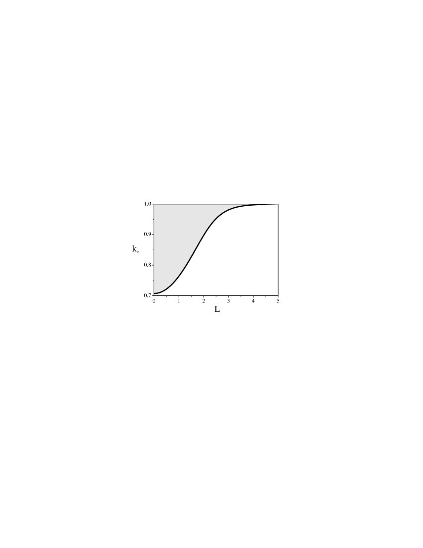
Figure 2: The dependence $k_{c}=k_{c}\left(L\right)$ (solid line). The stability region is shaded.

Substituting (21) into (6), we arrive at the expression for the current $J=J\left(L,k\right)$:

$$J=2k\sqrt{1-k^{2}}\frac{\text{sn}\left(L,k\right)}{\text{dn}\left(L,k\right)},\quad k\in\left[k_{c},1\right].$$ (28)

Note that for $L\equiv\frac{W}{2}\ll 1$ expression (28) reduces to the expected resultJ65 ; S72 ; BP82 ; L86

$$J\thickapprox\frac{W}{2}\sin\phi_{s}\left(0\right),$$ (29)

where, by (21) and (25),

$$\phi_{s}\left(0\right)=2\arccos k\in\left[0,\frac{\pi}{2}\right].$$

According to (28), the dependence $J_{c}=J_{c}\left(L\right)$ is given by

$$J_{c}=2k_{c}\sqrt{1-k_{c}^{2}}\frac{\text{sn}\left(L,k_{c}\right)}{\text{dn}\left(L,k_{c}\right)}.$$ (30)

Thus, for $L\equiv\frac{W}{2}\gg 1$, we get, using (26), (27),

$$J_{c}\thickapprox 2\left[1-8\exp\left(-W\right)\right].$$ (31)

For arbitrary $L\in\left(0,\infty\right)$, the dependence $J_{c}=J_{c}\left(L\right)$ is presented in Fig. 3. Although Fig. 3 reproduces the old resultsOS67 obtained by numerical maximization of $J$, we want to emphasize a substantial methodological difference: the curve $J_{c}=J_{c}\left(L\right)$ in Fig. 3 is nothing but a mapping by means of (30) of the boundary of the stability region $k_{c}=k_{c}\left(L\right)$ in Fig. 2.

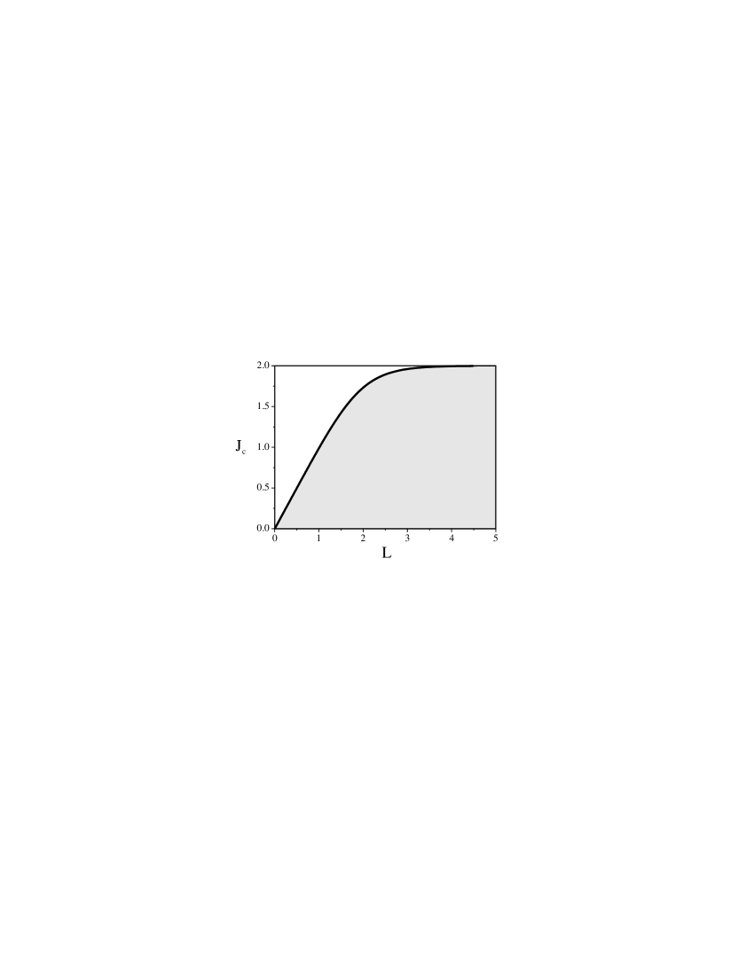
Figure 3: The dependence $J_{c}=J_{c}\left(L\right)$ for $H=0$ (solid line). The stability region is shaded.

III.1.2 The case $H\geq 0$, $J\geq 0$

For $H>0$, $J>0$, instead of (19), we have

$$\frac{d\phi}{dy}\left(-L\right)=\text{const},\quad\frac{d\phi}{dy}\left(-L\right)\neq\pm\frac{d\phi}{dy}\left(L\right).$$ (32)

Boundary conditions (32) break the symmetry (22). Taking into account that in the limit $H\rightarrow 0$ we must get (21), conditions (20) and (32) can be satisfied by

$$\phi_{s}\left(y\right)=2\arccos\left[k\,\frac{\text{cn}\left(y+\beta,k\right)}{\text{dn}\left(y+\beta,k\right)}\right],\quad k\in\left[k_{c},1\right),\quad\beta\in\left[0,\beta_{c}\right],$$ (33)

where $k_{c}$ is determined by (24), and $\beta_{c}\in\left[0,K\left(k\right)\right)$. The boundary of the stability region $\beta_{c}=\beta_{c}\left(k\right)$ is determined (see Appendix B) by the solution to the functional equation

$$\text{cn}\left(L+\beta_{c},k\right)\text{cn}\left(L-\beta_{c},k\right)\left[-E\left(L+\beta_{c},k\right)-E\left(L-\beta_{c},k\right)+\left(1-k^{2}\right)L\right]$$

$$+\left(1-k^{2}\right)\left[\text{sn}\left(L+\beta_{c},k\right)\text{cn}\left(L-\beta_{c},k\right)\text{dn}\left(L+\beta_{c},k\right)\right.$$

$$\left.+\text{sn}\left(L-\beta_{c},k\right)\text{cn}\left(L+\beta_{c},k\right)\text{dn}\left(L-\beta_{c},k\right)\right]=0,\quad k\in\left[k_{c},1\right),$$ (34)

under the condition $\beta_{c}\left(k_{c}\right)=0$.

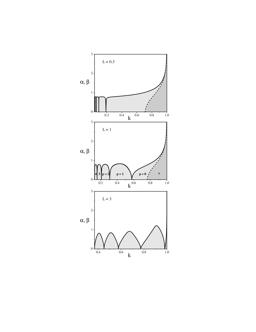
Figure 4: The stability regions of $\phi_{s}$ and $\phi_{p}$ ($p=0,1,2\ldots$) in the parametric plane (shaded) for $L=0.3,1,3$. The dependencies $\beta_{c}=\beta_{c}\left(k\right)$ and $\alpha_{c}=\alpha_{c}\left(k\right)$ are given by the dashed line and the solid lines, respectively.

In Fig. 4, we present the stability region of (33) obtained by numerical evaluation of Eq. (34) for several different values of $L$: $L=0.3$ (a ”small” junction), $L=1$ (a ”medium” junction), and $L=3$ (a ”large” junction). As we can see, $\lim_{k\rightarrow 1}\beta_{c}\left(k\right)\rightarrow\infty$. The asymptotics of $\beta_{c}\left(k\right)$ for $k\rightarrow 1$ can be established analytically.

Let us make the substitution

$$\beta_{c}=K\left(k\right)-\gamma_{c}$$ (35)

in Eq. (34). By proceeding to the limit $k=1$, we obtain a functional equation that determines the dependence $\gamma_{c}=\gamma_{c}\left(L\right)$ for $k=1$:

$$L\sinh\left(L-\gamma_{c}\right)\sinh\left(L+\gamma_{c}\right)-\frac{1}{2}\sinh^{2}\left(L-\gamma_{c}\right)\sinh\left(L+\gamma_{c}\right)\cosh\left(L-\gamma_{c}\right)$$

$$-\frac{1}{2}\sinh^{2}\left(L+\gamma_{c}\right)\sinh\left(L-\gamma_{c}\right)\cosh\left(L+\gamma_{c}\right)-\sinh\left(L+\gamma_{c}\right)\cosh\left(L-\gamma_{c}\right)-\sinh\left(L-\gamma_{c}\right)\cosh\left(L+\gamma_{c}\right)=0.$$ (36)

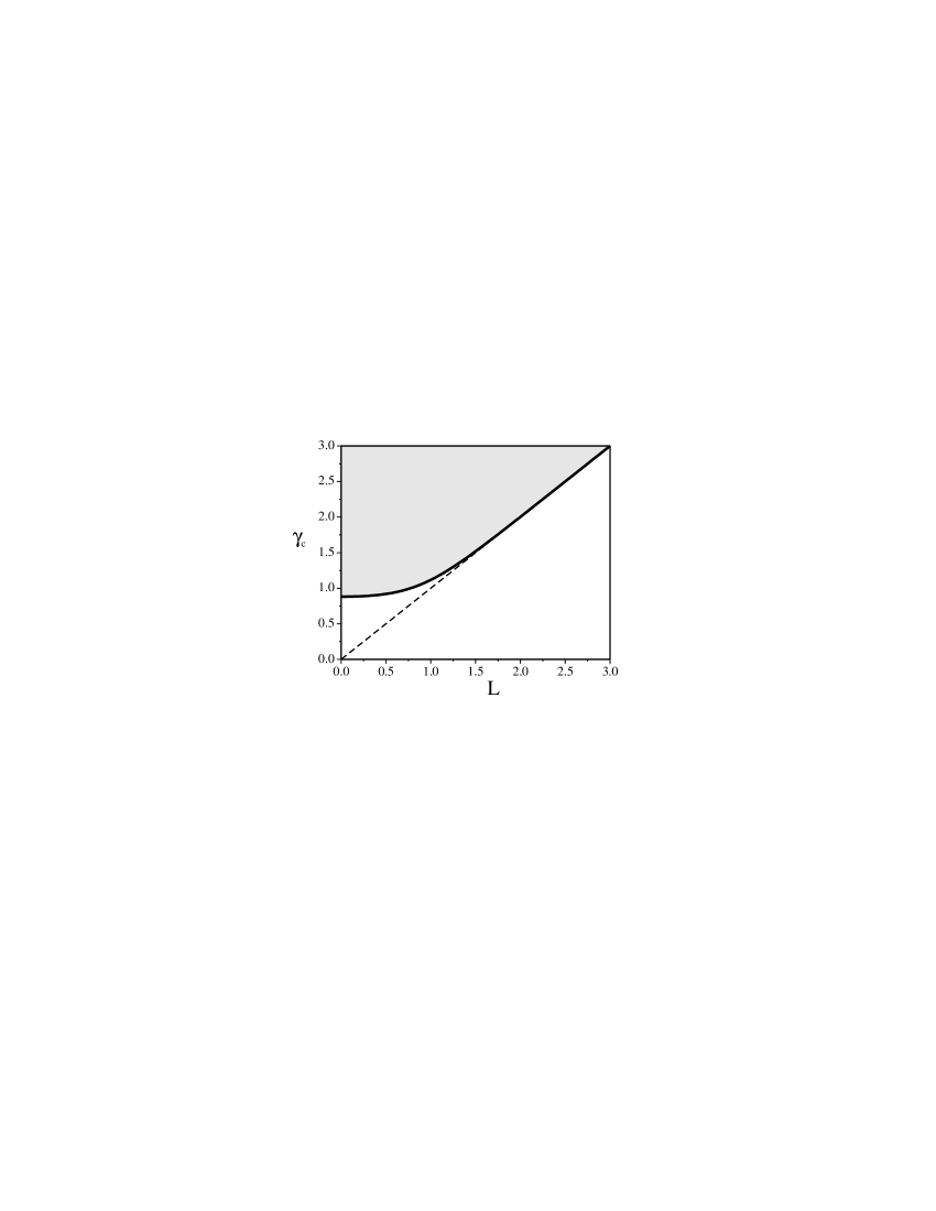
Figure 5: The dependence $\gamma_{c}=\gamma_{c}\left(L\right)$ (solid line). The stability region is shaded.

The numerical solution to this equation is given in Fig. 5. [Note that $\gamma_{c}\left(L\right)\thickapprox L$ for $L\gg 1$.] Taking into account relation (35), we arrive at the sought asymptotics of $\beta_{c}\left(k\right)$ for $k\rightarrow 1$:

$$\beta_{c}\left(k\right)\thickapprox\frac{1}{2}\ln\frac{16}{1-k^{2}}-\gamma_{c}\left(L\right).$$ (37)

Accordingly, the limiting form of the current-carrying solution (33) is

$$\lim_{k\rightarrow 1}\phi_{s}\left(y\right)\equiv\phi_{l}\left(y\right)=4\arctan\left[\exp\left(y-\gamma\right)\right],$$ (38)

where $\gamma\in\left[\gamma_{c},\infty\right)$ (see Fig. 5).

Equations (5) and (6), upon the substitution of (33), yield

$$H=\frac{k}{2}\sqrt{1-k^{2}}\left[\frac{\text{sn}\left(L+\beta,k\right)}{\text{dn}\left(L+\beta,k\right)}-\frac{\text{sn}\left(L-\beta,k\right)}{\text{dn}\left(L-\beta,k\right)}\right],$$ (39)

$$J=k\sqrt{1-k^{2}}\left[\frac{\text{sn}\left(L+\beta,k\right)}{\text{dn}\left(L+\beta,k\right)}+\frac{\text{sn}\left(L-\beta,k\right)}{\text{dn}\left(L-\beta,k\right)}\right],$$ (40)

$$k\in\left[k_{c},1\right),\quad\beta\in\left[0,\beta_{c}\right].$$

In the limit $k=1$, these relations take the form

$$H=\frac{\cosh L\cosh\gamma}{\cosh\left(\gamma-L\right)\cosh\gamma},$$ (41)

$$J=\frac{2\sinh L\sinh\gamma}{\cosh\left(\gamma-L\right)\cosh\gamma},\quad\gamma\in\left[\gamma_{c},\infty\right).$$ (42)

By setting $\beta=\beta_{c}$ in (39) and (40), we can obtain a relevant part of the dependence $J_{c}=J_{c}\left(H\right)$ for arbitrary $L\in\left(0,\infty\right)$: see Sec. IV.

We conclude the discussion of the solution $\phi_{s}$ by presenting an explicit analytical expression for the special case $J=2H$ that was the subject of numerical evaluation in Ref. ZhZ78 . From (39) and (40), we find: $\beta=L$. Substitution into (33) immediately yields

$$\left.\phi_{s}\left(y\right)\right|_{J=2H}=2\arccos\left[k\,\frac{\text{cn}\left(y+L,k\right)}{\text{dn}\left(y+L,k\right)}\right],\quad k\in\left[k_{m},1\right],$$ (43)

where $k_{m}$ is determined by the condition $\beta_{c}\left(k_{m}\right)=L$.

III.2 Solutions of type II

We start with the stable type-II solutions for the case $H\geq 0$, $J=0$:K04 ; K05 ; KG06

$$\phi_{p}(y)=\pi\left(p-1\right)+2\text{am}\left(\frac{y}{k}+K\left(k\right),k\right),\quad p=2m\quad\left(m=0,1,\ldots\right);$$ (44)

$$\phi_{p}(y)=\pi p+2\text{am}\left(\frac{y}{k},k\right),\quad p=2m+1\quad\left(m=0,1,\ldots\right),$$ (45)

where $\text{am }u$ is the Jacobian amplitude.AS65 The stability regions of (44), (45) are given by

$$p=0:k\in\left(k_{1},1\right);\quad p=1,2,\ldots:k\in\left(k_{p+1},k_{p}\right],$$ (46)

where the points $k=k_{p}$ ($p=1,2,\ldots$) are the roots of the equations

$$pk_{p}K\left(k_{p}\right)=L,\quad p=1,2,\ldots.$$ (47)

Solutions (44), (45) form an infinite set, and the union of their stability regions (46) (they interchange for even and odd $p$) is equal to the whole $k$-interval $\left(0,1\right)$. The meaning of the parameter $p=0,1,2,\ldots$ is revealed by the relation

$$p=\left\lfloor\frac{\phi_{p}\left(L\right)-\phi_{p}\left(-L\right)}{2\pi}\right\rfloor,$$ (48)

where $\left\lfloor\ldots\right\rfloor$ stands for the integer part of the argument.r3 Note also the symmetry property:

$$\phi_{p}\left(-y\right)=2\pi p-\phi_{p}\left(y\right).$$ (49)

For $H>0$, $J>0$, current-carrying type-II solutions obey the generalized boundary conditions (20), (32) that break the symmetry (49). These conditions can be satisfied if, in (44) and (45), we make a shift of the argument $y\rightarrow y+k\alpha$ (with $\alpha$ being a new parameter):

$$\phi_{p}(y)=\pi\left(p-1\right)+2\text{am}\left(\frac{y}{k}+K\left(k\right)+\alpha,k\right),\quad\alpha\in\left[0,\alpha_{c}\right],\quad p=2m\quad\left(m=0,1,\ldots\right);$$ (50)

$$\phi_{p}(y)=\pi p+2\text{am}\left(\frac{y}{k}+\alpha,k\right),\quad\alpha\in\left[0,\alpha_{c}\right],\quad p=2m+1\quad\left(m=0,1,\ldots\right).$$ (51)

The domains of the parameter $k$ in (50) and (51) are given by (46), (47), whereas $\alpha_{c}\in\left[0,K\left(k\right)\right)$. The boundaries of the stability regions $\alpha_{c}=\alpha_{c}\left(k\right)$ are determined (see Appendix B) by the solutions to the functional equation

$$k^{2}\text{sn}\left(\frac{L}{k}+\alpha_{c},k\right)\text{sn}\left(\frac{L}{k}-\alpha_{c},k\right)\text{cn}\left(\frac{L}{k}+\alpha_{c},k\right)\text{cn}\left(\frac{L}{k}-\alpha_{c},k\right)\left[E\left(\frac{L}{k}+\alpha_{c},k\right)+E\left(\frac{L}{k}-\alpha_{c},k\right)\right]$$

$$+\text{sn}\left(\frac{L}{k}-\alpha_{c},k\right)\text{cn}\left(\frac{L}{k}-\alpha_{c},k\right)\text{dn}^{3}\left(\frac{L}{k}+\alpha_{c},k\right)+\text{sn}\left(\frac{L}{k}+\alpha_{c},k\right)\text{cn}\left(\frac{L}{k}+\alpha_{c},k\right)\text{dn}^{3}\left(\frac{L}{k}-\alpha_{c},k\right)=0$$ (52)

in the case (50), and to the functional equation

$$\frac{k^{2}}{1-k^{2}}\text{sn}\left(\frac{L}{k}+\alpha_{c},k\right)\text{sn}\left(\frac{L}{k}-\alpha_{c},k\right)\text{cn}\left(\frac{L}{k}+\alpha_{c},k\right)\text{cn}\left(\frac{L}{k}-\alpha_{c},k\right)$$

$$\times\left\{E\left(\frac{L}{k}+\alpha_{c},k\right)+E\left(\frac{L}{k}-\alpha_{c},k\right)-k^{2}\left[\frac{\text{sn}\left(\frac{L}{k}+\alpha_{c},k\right)\text{cn}\left(\frac{L}{k}+\alpha_{c},k\right)}{\text{dn}\left(\frac{L}{k}+\alpha_{c},k\right)}+\frac{\text{sn}\left(\frac{L}{k}-\alpha_{c},k\right)\text{cn}\left(\frac{L}{k}-\alpha_{c},k\right)}{\text{dn}\left(\frac{L}{k}-\alpha_{c},k\right)}\right]\right\}$$

$$-\frac{\text{sn}\left(\frac{L}{k}-\alpha_{c},k\right)\text{cn}\left(\frac{L}{k}-\alpha_{c},k\right)}{\text{dn}\left(\frac{L}{k}+\alpha_{c},k\right)}-\frac{\text{sn}\left(\frac{L}{k}+\alpha_{c},k\right)\text{cn}\left(\frac{L}{k}+\alpha_{c},k\right)}{\text{dn}\left(\frac{L}{k}-\alpha_{c},k\right)}=0$$ (53)

in the case (51). The relevant solutions to (52) and (53) must satisfy the conditions $\alpha_{c}\left(k_{p}\right)=0$ ($p=1,2,\ldots$).

Making the substitution

$$\alpha_{c}=K\left(k\right)-\gamma_{c}$$ (54)

and proceeding to the limit $k=1$ in Eq. (52) with $p=0$, we arrive at Eq. (36). Accordingly, for $k\rightarrow 1$, the asymptotics of $\alpha_{c}\left(k\right)$ coincides with that of $\beta_{c}\left(k\right)$ [relation (37)]:

$$\alpha_{c}\left(k\right)\thickapprox\frac{1}{2}\ln\frac{16}{1-k^{2}}-\gamma_{c}\left(L\right),$$ (55)

where the dependence $\gamma_{c}=\gamma_{c}\left(L\right)$ is represented by the graph in Fig. 5. The feature (55) is clearly reproduced in Fig. 4, where we present the stability regions of (50) and (51) obtained by numerical evaluation of (52) and (53), respectively, for $L=0.3,1,3$. Moreover, as could by expected from the general arguments at the beginning of this section, the limiting form ($k=1$) of the current-carrying solution (50) for $p=0$ coincides with the limiting form ($k=1$) of the current-carrying solution (33), i.e.,

$$\lim_{k\rightarrow 1}\phi_{0}=\lim_{k\rightarrow 1}\phi_{s}=\phi_{l},$$

where $\phi_{l}=\phi_{l}\left(y\right)$ is given by (38).

It is interesting to note that equations (52) and (53) have exact analytical solutions at the points $k=k_{p}^{\ast}$ ($p=0,1,2,\ldots$), where $k_{p}^{\ast}$ are implicitly determined by the equations

$$\left(p+\frac{1}{2}\right)k_{p}^{\ast}K\left(k_{p}^{\ast}\right)=L,\quad p=0,1,2,\ldots.$$ (56)

Namely,

$$\alpha_{c}\left(k_{p}^{\ast}\right)=\frac{1}{2}K\left(k_{p}^{\ast}\right),\quad p=0,1,2,\ldots.$$ (57)

The role of these solutions is discussed in Sec. IV.

Upon the substitution of (50) and (51) into (5) and (6), we obtain, respectively,

$$H=\frac{\sqrt{1-k^{2}}}{2k}\left[\text{dn}^{-1}\left(\frac{L}{k}+\alpha,k\right)+\text{dn}^{-1}\left(\frac{L}{k}-\alpha,k\right)\right],$$ (58)

$$J=\frac{\sqrt{1-k^{2}}}{k}\left[\text{dn}^{-1}\left(\frac{L}{k}+\alpha,k\right)-\text{dn}^{-1}\left(\frac{L}{k}-\alpha,k\right)\right],$$ (59)

$$\alpha\in\left[0,\alpha_{c}\right],$$

for the case (50) ($p=2m$, $m=0,1,\ldots$), and

$$H=\frac{1}{2k}\left[\text{dn}\left(\frac{L}{k}+\alpha,k\right)+\text{dn}\left(\frac{L}{k}-\alpha,k\right)\right],$$ (60)

$$J=\frac{1}{k}\left[\text{dn}\left(\frac{L}{k}+\alpha,k\right)-\text{dn}\left(\frac{L}{k}-\alpha,k\right)\right],$$ (61)

$$\alpha\in\left[0,\alpha_{c}\right],$$

for the case (51) ($p=2m+1$, $m=0,1,\ldots$), with the domains of the parameter $k$ being determined by (46), (47). In the limit $k=1$, equations (58), (59) for $p=0$ take the form (41), (42), as they should.

By setting $\alpha=\alpha_{c}$ in (58)-(61), we can obtain relevant parts of the dependence $J_{c}=J_{c}\left(H\right)$ for arbitrary $L\in\left(0,\infty\right)$: this is the subject of the next section. However, we want to conclude this section by demonstrating how the above exact analytical results reproduce the well-knownJ65 ; S72 ; BP82 ; L86 ”Fraunhofer pattern” of $J_{c}=J_{c}\left(H\right)$ in the limiting case $L\equiv\frac{W}{2}\ll 1$.

In the case $L\ll 1$, the solutions to Eqs. (47) are

$$k_{p}\thickapprox\frac{2L}{p\pi}\ll 1,\quad p=1,2,\ldots$$ (62)

(see Fig. 4 for $L=0.3$). Accordingly, the domains of the parameter $k$ [relations (46)] become

$$p=0:k\in\left(\frac{2L}{\pi},1\right);\quad p=1,2,\ldots:k\in\left(\frac{2L}{\left(p+1\right)\pi},\frac{2L}{p\pi}\right].$$ (63)

Therefore, we focus our attention on the case $k\ll 1$. In this limit, for $k\neq k_{p}$ ($p=1,2,\ldots$), the solution to both Eq. (52) and  Eq. (53) is

$$\alpha_{c}\thickapprox\frac{\pi}{4}.$$ (64)

For $k\ll 1$, equations (58) and (60) yield

$$k\thickapprox H^{-1},$$ (65)

whereas Eqs. (59), (61) become

$$J\thickapprox\left(-1\right)^{p}\frac{k}{2}\sin\left(\frac{2L}{k}\right)\sin\left(2\alpha\right),\quad\alpha\in\left[0,\frac{\pi}{4}\right];\quad p=0,1,2,\ldots.$$ (66)

Combining relations (63)-(66), we arrive at an approximate dependence $J\thickapprox J\left(H,\alpha\right)$ for $L\equiv\frac{W}{2}\ll 1$:

$$J\thickapprox\frac{1}{2H}\left|\sin\left(HW\right)\right|\sin\left(2\alpha\right),\quad\alpha\in\left[0,\frac{\pi}{4}\right].$$ (67)

As a result,

$$J_{c}\left(H\right)\thickapprox\frac{1}{2H}\left|\sin\left(HW\right)\right|.$$ (68)

Our derivation clearly reveals limitations of the approximate relation (68) (the ”Fraunhofer pattern”): strictly speaking, in the field range $0<H\lesssim 1$ (i.e., when $k\rightarrow 1$), it can be regarded, at most, as a reasonable interpolation. Moreover, the approximation (68) breaks down near the boundaries of the stability regions $H\thickapprox\frac{p\pi}{W}$, $p=1,2,\ldots$, (i.e., when $k\thickapprox k_{p}$). Unfortunately, these limitations are not accounted for in elementary derivationsJ65 ; S72 ; BP82 ; L86 of (68).

Finally, we note that, as is clear from (65), the actual expansion parameter in relations (66)-(68) is $H^{-1}\ll 1$ rather than $L\ll 1$. Therefore, for $H\gg 1$, the approximation (68) is valid for arbitrary $W\in\left(0,\infty\right)$. (This fact was first pointed out in Ref. Zh78 .) For reference purposes, we present the corresponding ($H\gg 1$) asymptotics of the current-carrying solutions $\phi_{p}$:

$$\phi_{p}\left(y\right)\thickapprox p\pi+2Hy+2\alpha-\frac{\alpha}{2H^{2}}-\frac{\left(-1\right)^{p}}{4H^{2}}\left[\sin\left(2Hy+2\alpha\right)-2Hy\cos\left(HW\right)\cos\left(2\alpha\right)\right],$$ (69)

$$\alpha\in\left[0,\frac{\pi}{4}\right];\quad p=0:H\in\left(1,\frac{\pi}{W}\right);\quad p=1,2,\ldots:H\in\left(\frac{p\pi}{W},\frac{\left(p+1\right)\pi}{W}\right).$$

IV Major physical results

IV.1 Stability regions in the plane $\left(H,J\right)$ and the dependence $J_{c}=J_{c}\left(H\right)$

Relations (39), (40) and (58)-(61) map the stability regions of the current-carrying solutions (33) and (50), (51), respectively, from the parametric planes $\left(\beta,k\right)$, $\left(\alpha,k\right)$ to the physical plane $\left(H,J\right)$. In Fig. 6, we present the results of this mapping for the data of Fig. 4. As already noted (Sec. III), the boundaries of the stability regions represent the dependence $J_{c}=J_{c}\left(H\right)$ that consists of an infinite number of separate branches.

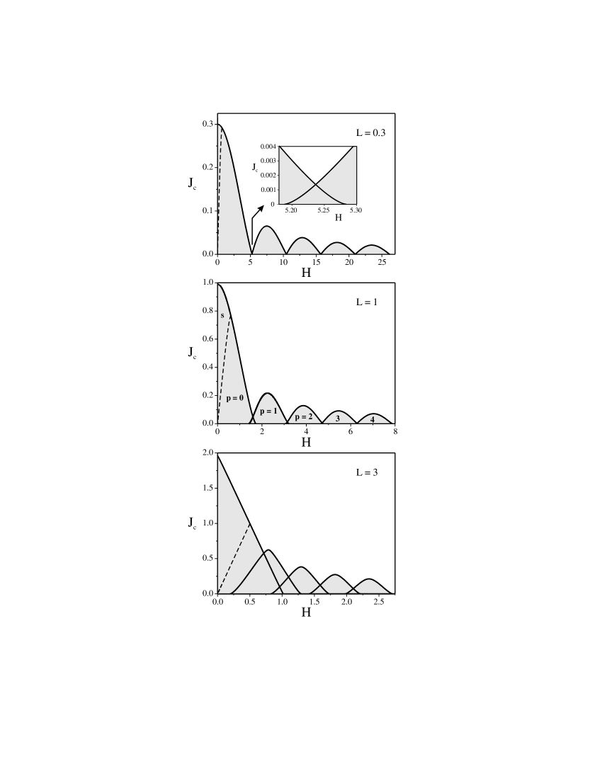
Figure 6: The stability regions of $\phi_{s}$ and $\phi_{p}$ ($p=0,1,2\ldots$) in the physical plane $\left(H,J\right)$ (shaded) for $L=0.3,1,3$. The dependence $J_{c}=J_{c}\left(H\right)$ is given by the solid lines. The dashed line represents the internal boundary where $\phi_{s}=\phi_{0}=\phi_{l\text{.}}$.

As can be easily seen, the structure of the stability regions [including the boundaries $J_{c}=J_{c}\left(H\right)$] is qualitatively the same for all the considered cases: $L=0.3$ (a ”small” junction), $L=1$ (a ”medium” junction), and $L=3$ (a ”large” junctions). Thus, as the solutions $\phi_{s}$ [Eq. (33)] and $\phi_{0}$ [Eq. (50)] constitute two different branches of the same current-carrying solution, their stability regions (labeled by the indices $s$ and $p=0$, respectively) merge to form a unified stability domain. The transformation $\phi_{s}\longleftrightarrow\phi_{0}$ occurs on the internal boundary (41), (42) (represented by the dashed line in Fig. 6), where these two solutions coincide with the elementary solution $\phi_{l}$ [Eq. (38)].

The stability regions corresponding to $\phi_{p=2m}$ and $\phi_{p=2m+1}$ interchange and form an infinite set. Significantly, for arbitrary $L\in\left(0,\infty\right)$, each two consecutive stability regions, labeled by $p$ and $p+1$, overlap in the field range

$$\sqrt{H_{p}^{2}-1}\leq H<H_{p},$$ (70)

where $H_{p}$ are the roots of

$$\left(p+1\right)K\left(\frac{1}{H_{p}}\right)=H_{p}L,\quad p=0,1,2,\ldots.$$ (71)

Indeed, for $J=0$, the stability regions of the solutions $\phi_{p}$ [Eqs. (44), (45)] are given by the field intervalsKG06

$$p=0:0\leq H<H_{0};$$ (72)

$$p=1,2,\ldots:\sqrt{H_{p-1}^{2}-1}\leq H<H_{p};$$ (73)

hence relation (70). Moreover, for sufficiently large $L$, the overlap may involve several consecutive stability regions: see Fig. 6 for $L=3$. In contrast, the overlap decreases with an increase in $p$ and a decrease in $L$: see the insert in Fig. 6 for $L=0.3$. The overlap of the stability regions results in multivaluedness of the dependence $J_{c}=J_{c}\left(H\right)$.

For $L\gtrsim 1$, the multivaluedness of $J_{c}=J_{c}\left(H\right)$ was found by numerical evaluation.OS67 However, the fact that this multivaluedness is an intrinsic feature of any Josephson junction (even with $L\ll 1$) was not noticed because of the absence of exact analytical solutions.

IV.2 Unquantized Josephson vortices

In contrast to the case $J=0$,r3 the discrete parameter $p$ of the exact solutions (50) and (51) for $J>0$ cannot be identified with the number of Josephson vortices, although relation (48) still holds. The reason is the occurrence (for certain values of $H$ and $J$) of unquantized vortices carrying fractional flux $\Phi\in\left(\frac{1}{2}\Phi_{0},\Phi_{0}\right)$, where $\Phi_{0}$ is the flux quantum. (In our dimensionless units, $\Phi_{0}=\pi$.) To clarify the situation, we should consider spatial distribution of the local magnetic field $h$ and of the Josephson current density $j$ for $J=J_{c}$.

As follows from (1) and (3), the local magnetic field $h$ obeys the linear homogeneous second-order differential equation

$$\frac{d^{2}h}{dy^{2}}=\cos\phi\left(y\right)h.$$ (74)

Combining Eq. (74) and Eqs. (10), (11) for the boundary of the stability region, we obtain

$$\bar{\psi}_{0}\left(L\right)\frac{dh}{dy}\left(L\right)=\bar{\psi}_{0}\left(-L\right)\frac{dh}{dy}\left(-L\right).$$ (75)

Taking into account (12), we find that either

$$\frac{dh}{dy}\left(L\right)=\frac{dh}{dy}\left(-L\right)=0,$$ (76)

or

$$\frac{dh}{dy}\left(L\right)\frac{dh}{dy}\left(-L\right)>0.$$ (77)

The solution $\phi_{s}$ [Eq. (33)] satisfies relation (77) everywhere on the critical curve $J_{c}=J_{c}\left(H\right)$. Moreover, for this solution, $\frac{dh}{dy}\left(y\right)>0$ for any $y\in\left[-L,L\right]$. [Accordingly, $j\left(y\right)>0$ for any $y\in\left[-L,L\right]$: see (2) and (3).]

The behavior of $\phi_{p}$ [Eqs. (50) and (51)] is more complicated. First, we note that $\phi_{p}$ satisfy (76) at those values of $H$ for which $J_{c}=0$. This occurs at $H=H_{0}$ (for $\phi_{0}$) and at $H=\sqrt{H_{p-1}^{2}-1},H_{p}$ (for $\phi_{p}$with $p=1,2,\ldots$), where $H_{p}$ are determined by (71): as a matter of fact, this case has been considered in detail in Ref. KG06 .

In addition, relation (76) is satisfied by $\phi_{p}$ at such fields $H=H_{p}^{\ast}$ ($p=0,1,2,\ldots$) that $J_{c}=\left(2H_{p}^{\ast}\right)^{-1}$. These fields are given by

$$H_{p}^{\ast}=\frac{1}{2k_{p}^{\ast}}\left[1+\sqrt{1-\left(k_{p}^{\ast}\right)^{2}}\right],\quad p=0,1,2,\ldots,$$

where $k_{p}^{\ast}$ are determined by (56). At $H=H_{p}^{\ast}$, we have: $\phi_{p}\left(-L\right)=0$, $\phi_{p}\left(L\right)=\pi\left(2p+1\right)$.

At the rest of the points on the critical curves $J_{c}=J_{c}\left(H\right)$, the solutions $\phi_{p}$ ($p=0,1,2,\ldots$) satisfy (77). In particular, we have: (a) $\frac{dh}{dy}\left(\pm L\right)>0$ for $H<H_{p}^{\ast}$ ($p=0,1,2,\ldots$), because $\phi_{p}\left(-L\right)\in\left(0,\frac{\pi}{2}\right)$ and $\phi_{p}\left(L\right)\in\left(2\pi p,2\pi\left(p+\frac{1}{2}\right)\right)$; (b) $\frac{dh}{dy}\left(\pm L\right)<0$ for $H>H_{p}^{\ast}$ ($p=0,1,2,\ldots$), because $\phi_{p}\left(-L\right)\in\left(-\pi,0\right)$ and $\phi_{p}\left(L\right)\in\left(2\pi\left(p+\frac{1}{2}\right),2\pi\left(p+1\right)\right)$.

To establish the types of Josephson-vortex structures that are represented by the solutions $\phi_{p}$ ($p=0,1,2,\ldots$) on the critical curve $J_{c}=J_{c}\left(H\right)>0$, we have to classify the points of local minima of $h$. Thus, for $H<H_{p}^{\ast}$ ($p=0,1,2,\ldots$), the first minimum is positioned at $y=-L$, where $\frac{dh}{dy}\left(-L\right)>0$. The rest of the minima (for $p>0$) are positioned at $y=y_{n}$ ($n=1,\ldots,p$), where $\phi_{p}\left(y_{n}\right)=2\pi n$ and $\frac{dh}{dy}\left(y_{n}\right)=0$.

For $H=H_{p}^{\ast}$ ($p=0,1,2,\ldots$), the first minimum is positioned at $y=-L$, where $\phi_{p}\left(-L\right)=0$ and $\frac{dh}{dy}\left(-L\right)=0$. The rest of the minima (For $p>0$) are positioned at $y=y_{n}$ ($n=1,\ldots,p$), where $\phi_{p}\left(y_{n}\right)=2\pi n$ and $\frac{dh}{dy}\left(y_{n}\right)=0$.

For $H>H_{p}^{\ast}$ ($p=0,1,2,\ldots$), we have a minimum at $y=L$, where $\frac{dh}{dy}\left(L\right)<0$. The rest of the minima are positioned at $y=y_{n}$ ($n=0,\ldots,p$), where $\phi_{p}\left(y_{n}\right)=2\pi n$ and $\frac{dh}{dy}\left(y_{n}\right)=0$.

Bearing in mind that a Josephson vortex is located between two consecutive local minima of $h$,KG06 we arrive at the following physical interpretation of $\phi_{p}$:

(i) $H<H_{p}^{\ast}$ ($p=0,1,2,\ldots$). The solution $\phi_{0}$ represents a vortex-free configuration. The solutions labeled by $p=1,2,\ldots$ represent configurations with $p-1$ quantized Josephson vortices located between the points $y_{n}$, $y_{n+1}$ ($n=1,\ldots,p-1$) and carrying flux $\Phi=\Phi_{0}$. In addition, these configurations contain a single unquantized vortex carrying flux $\Phi\in\left(\frac{1}{2}\Phi_{0},\Phi_{0}\right)$ and located between $y=-L$ and $y=y_{1}$;

(ii) $H=H_{p}^{\ast}$ ($p=0,1,2,\ldots$). The solution $\phi_{0}$ represents a vortex-free configuration. The solutions labeled by $p=1,2,\ldots$ represent configurations with $p$ quantized Josephson vortices located between the points $y=-L$, $y_{1}$, and $y_{n}$, $y_{n+1}$ ($n=1,\ldots,p-1$; $p>1$);

(iii) $H>H_{p}^{\ast}$ ($p=0,1,2,\ldots$). The solutions labeled by $p=1,2,\ldots$ represent configurations with $p$ quantized Josephson vortices located between the points $y_{n}$, $y_{n+1}$ ($n=0,\ldots,p-1$).  In addition, all these configurations ($p=0,1,2,\ldots$) contain a single unquantized vortex located between $y_{p}$ and $y=L$.

The above general analytical conclusions are illustrated in Figs. 7 and 8. For simplicity, in Fig. 7, we restrict ourselves to the first two critical curves $J_{c}=J_{c}\left(H\right)$ of the junction with $L=1$. Spatial distribution of $h$ and $j$ at typical points 0-7 on these curves is presented in Fig. 8, were we also mark the locations of both quantized and unquantized Josephson vortices.

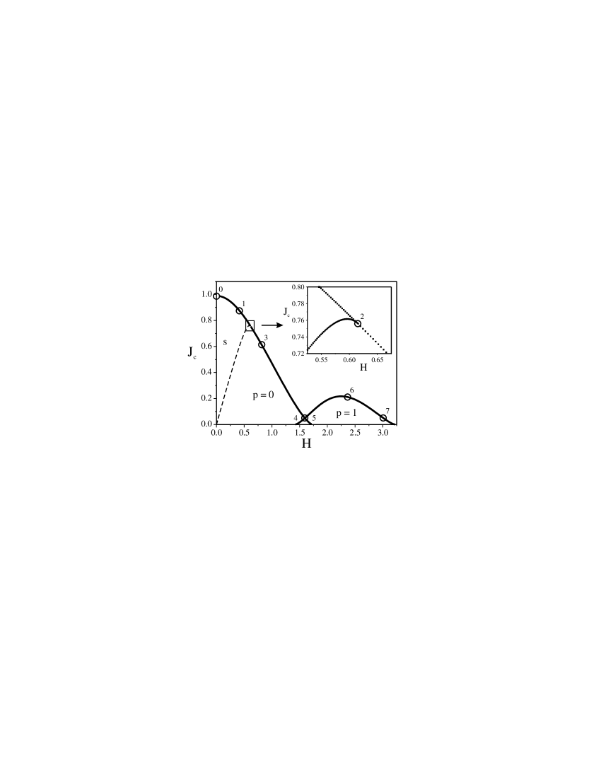
Figure 7: The first two critical curves $J_{c}=J_{c}\left(H\right)$ for $L=1$. Spatial distribution of $h$ and $j$ (Fig. 8) is evaluated at typical points 0-7: (0) $H=0.00$, $J_{c}=0.99$; (1) $H=0.43$, $J_{c}=0.87$; (2) $H=0.61$, $J_{c}=0.76$ ($\phi_{s}=\phi_{0}=\phi_{l\text{.}}$); (3) $H=H_{0}^{\ast}=0.81$, $J_{c}=\left(2H_{0}^{\ast}\right)^{-1}=0.61$; (4) $H=1.60$, $J_{c}=0.05$ (the first curve); (5) $H=1.60$, $J_{c}=0.05$ (the second curve); (6) $H=H_{1}^{\ast}=2.36$, $J_{c}=\left(2H_{1}^{\ast}\right)^{-1}=0.21$; (7) $H=3.01$, $J_{c}=0.05$.

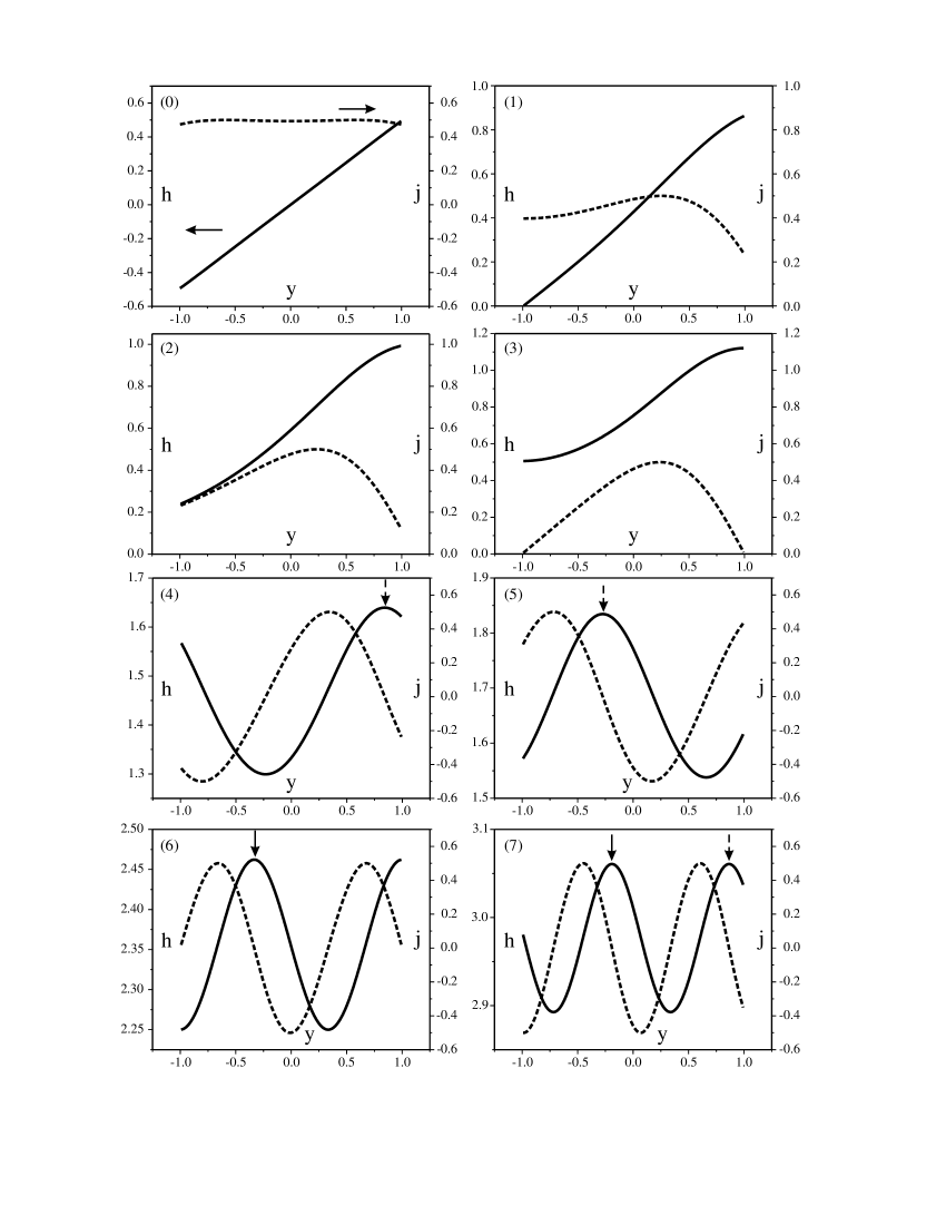
Figure 8: Spatial distribution of $h$ (solid line) and $j$ (dashed line) for points 0-7 in Fig. 7. The location of Josephson vortices is marked by vertical arrows: the dashed arrows correspond to unquantized vortices [figures (4), (5) and (7)]; the solid arrows correspond to quantized vortices [figures (6) and (7)].

In conclusion, we want to emphasize that, as follows from continuity arguments, unquantized Josephson vortices persist in certain two-dimensional domains on the plane $\left(H,J\right)$, where $J<J_{c}$. Therefore, the existence of such vortices is a typical feature of any Josephson junction in the presence of externally applied magnetic fields and transport currents.

IV.3 Generalizations

The restriction $H\geq 0$, $J\geq 0$ imposed at the beginning of Sec. III can be easily removed. Physical solutions that do not obey these restriction are expressed via the solutions $\phi_{s}$, $\phi_{p}$ and $\phi_{l}$ [Eqs. (33), (50), (51), and (38), respectively] by means of elementary symmetry relations.

1. The case $H\leq 0$, $J\geq 0$:

$$\phi_{s},\beta\rightarrow\phi_{s},-\beta;\qquad\phi_{p},\alpha\rightarrow-\phi_{p},-\alpha;\qquad\phi_{l},\gamma\rightarrow 2\pi-\phi_{l},-\gamma.$$ (78)

2. The case $H\geq 0$, $J\leq 0$:

$$\phi_{s},\beta\rightarrow-\phi_{s},-\beta;\qquad\phi_{p},\alpha\rightarrow\phi_{p},-\alpha;\qquad\phi_{l},\gamma\rightarrow\phi_{l}-2\pi,-\gamma.$$ (79)

3. The case $H\leq 0$, $J\leq 0$:

$$\phi_{s},\beta\rightarrow-\phi_{s},\beta;\qquad\phi_{p},\alpha\rightarrow-\phi_{p},\alpha;\qquad\phi_{l},\gamma\rightarrow-\phi_{l},\gamma.$$ (80)

Finally, we note that the consideration of this paper equally applies to a generalized form of the boundary conditions that takes into account possible asymmetry in the injection of the transport current, namely,BP82 ; L86

$$\frac{d\phi}{dy}\left(\pm L\right)=2\left(H\pm a_{\mp}J\right),$$ (81)

or, equivalently,

$$H=\frac{1}{2}\left[a_{+}\frac{d\phi}{dy}\left(+L\right)+a_{-}\frac{d\phi}{dy}\left(-L\right)\right],$$

$$J=\frac{1}{2}\left[\frac{d\phi}{dy}\left(+L\right)-\frac{d\phi}{dy}\left(-L\right)\right].$$

where

$$a_{\pm}\geq 0,\quad a_{-}+a_{+}=1.$$

The effect of the generalized boundary conditions (81) is illustrated in Fig. 9.

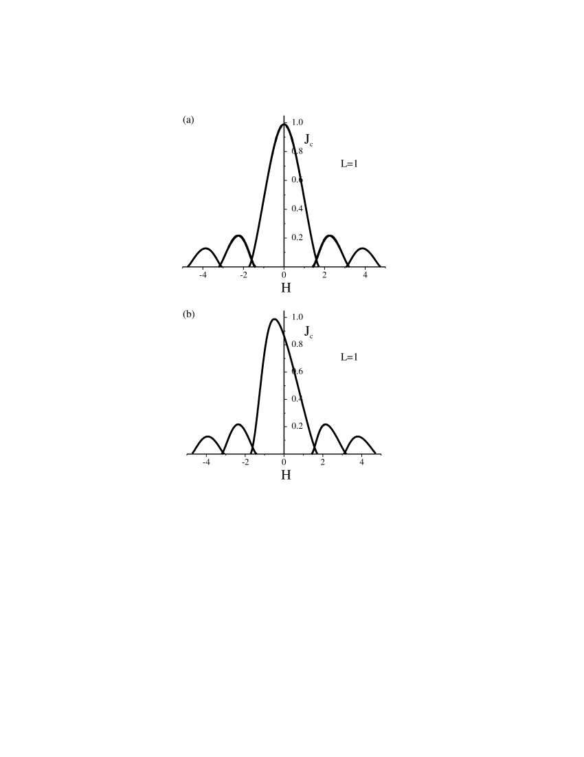
Figure 9: The effect of asymmetric injection of the transport current on the dependence $J_{c}=J_{c}\left(H\right)$ for $L=1$: (a) $a_{\pm}=\frac{1}{2}$; (b) $a_{+}=0$, $a_{-}=1$.

V Summary and conclusions

Summarizing, we have derived the complete set of exact physical solutions to the general boundary-value problem (3), (81): $\phi_{s}$ [Eq. (33)] and $\phi_{p}$ ($p=0,1,2,\ldots$) [Eqs. (50), (51)] complemented by the symmetry relations (78)-(80). The obtained solutions describe the current-carrying states of the Josephson junction of arbitrary length $W\equiv 2L\in\left(0,\infty\right)$ in the presence of an externally applied magnetic field $H\in\left(-H_{c},H_{c}\right)$, where $H_{c}$ is the thermodynamic critical field of the superconducting electrodes. The most direct application of these solutions is straightforward evaluation of the dependence $J_{c}=J_{c}\left(H\right)$ (for arbitrary $W$ and an arbitrary mode of the injection of $J$) by means of the algorithm of Secs. III and IV.

Mathematically, $\phi_{s}$ and $\phi_{p}$ ($p=0,1,2,\ldots$) represent the complete set of particular solutions to (3) that are stable under the condition that $\frac{d\phi}{dy}$ is fixed at the boundaries $y=\pm L$, and they possess a number of interesting properties. For example, the solutions $\phi_{s}$ and $\phi_{0}$ constitute two different branches of the same stable solution: for $k\rightarrow 1$, both of them turn into the elementary solution $\phi_{l}$ [Eq. (38)]. In physical literature,S72 ; BP82 ; L86 the elementary solution $\phi_{l}$ is usually identified with ”the Josephson vortex”. Indeed, if Eq. (3) were considered on the infinite interval $\left(-\infty,\infty\right)$, this solution would be nothing but the well-knownDEGM82 static soliton of the sine-Gordon equation, positioned at $y=\gamma$ and stable for arbitrary $\left|\gamma\right|<\infty$. However, on the physically realistic finite interval $\left[-L,L\right]$, the solution $\phi_{l}$ proves to be stable only for $\left|\gamma\right|\geq\gamma_{c}$, where $\gamma_{c}$ is determined by Eq. (36), and, as shown in Sec. IV, it has nothing to do with any vortex (or soliton) configurations.

As could be anticipated, the exact analytical solution of the problem that remained unresolved for over four decades has revealed some unexpected physical features. For example, contrary to a wide-spread belief,S72 ; BP82 ; L86 it clearly shows that there is no qualitative difference between Josephson junctions with $W\gg 1$ and those with $W\ll 1$. Thus, the exact analytical dependence $J_{c}=J_{c}\left(H\right)$ proves to be multivalued even for arbitrarily small $W$. Therefore, hysteresis is an intrinsic feature of any Josephson junction with $W\in\left(0,\infty\right)$.

However, we think that the most important physical conclusion that can be drawn from the exact analytical solution is the existence of unquantized Josephson vortices. Indeed, recently, the possibility of finding unquantized vortices in different types of superconducting systems (including Josephson ones) has attracted considerable attention: see, e.g., Refs. B02 ; Mi02  and references therein. In most theoretical models, unquantized vortices appear as a result of unconventional properties of the superconductors themselves, such as, e.g., the existence of two superconducting order parameters,B02 $d$-wave pairing combined with the inhomogeneity of grain boundaries,Mi02 etc. By contrast, we have shown that the presence of unquantized Josephson vortices near the external boundaries is a typical feature of any classical Josephson junction, provided the transport current $J$ is sufficiently close to $J_{c}$ for certain finite values of $H$.

From a mathematical point of view, it would be desirable to know whether the quantity $J_{\max}$ discussed in the Introduction indeed coincides with $J_{c}$ evaluated in this paper. Although we have been unable to find a general analytical proof, our detailed comparisons with the numerical results of Refs. OS67 ; BB75 (not presented here for brevity reasons) imply that the identity $J_{\max}\equiv J_{c}$ can be accepted without reservation.

Finally, we want to remind once again that Eq. (3) is just the static version of the well-known sine-Gordon equation [Eq. (82) with $\kappa=0$]. Given that the sine-Gordon equation finds a lot of applications in condensed-matter and elementary-particle physics,DEGM82 we hope that our exact analytical solution may find applications outside the field of superconductivity as well.

Acknowledgements

We thank A. N. Omelyanchouk, A. S. Kovalev, and M. M. Bogdan for stimulating discussions of the main physical and mathematical results of the paper.

Appendix A Alternative formulation of the stability problem

The stability of a given solution $\phi=\phi\left(y\right)$ to (3), (4) can also be analyzed using the general time-dependent equationBP82

$$\frac{\partial^{2}\phi}{\partial t^{2}}+2\kappa\frac{\partial\phi}{\partial t}-\frac{\partial^{2}\phi}{\partial y^{2}}+\sin\phi=0,$$ (82)

where $\kappa>0$, $t\geq 0$ and $y\in\left(-L,L\right)$, under the boundary conditions

$$\frac{d\phi}{dt}\left(t,\pm L\right)=2H\pm J.$$ (83)

According to linear stability theory,JJ80 we should seek solutions to (82), (83) in the form

$$\tilde{\phi}\left(t,y\right)=\phi\left(y\right)+e^{-\sigma t}\zeta\left(y\right),$$ (84)

where

$$\max_{y}\left|\zeta\left(y\right)\right|\ll 1,$$

and

$$\frac{d\zeta}{dy}\left(\pm L\right)=0.$$ (85)

Substituting (84) into (82) and dropping nonlinear terms, we obtain:

$$-\frac{d^{2}\zeta}{dy^{2}}+\cos\phi\left(y\right)\zeta=\sigma\left(2\kappa-\sigma\right)\zeta.$$ (86)

Equation (86) under boundary conditions (85) immediately yields

$$\sigma_{n\pm}=\kappa\pm\sqrt{\kappa^{2}-\mu_{n}},\quad n=0,1,2,\ldots,$$ (87)

where $\mu_{0}<\mu_{1}<\mu_{2}<\ldots$ are the eigenvalues of the Sturm-Liouville problem (8), (9). Thus, we arrive at the following classification of stability properties of the solution $\phi=\phi\left(y\right)$:

i) $\mu_{0}>0$, $\text{Re }\sigma_{n\pm}>0$ ($n=0,1,2,\ldots$): the solution is exponentially stable;

ii) $\mu_{0}<0$, $\sigma_{0-}=\kappa-\sqrt{\kappa^{2}+\left|\mu_{0}\right|}<0$: the solution is unstable;

iii) $\mu_{0}=0$, $\sigma_{0-}=0$: the solution is at the boundary of the stability region.

Appendix B Solution of the linear boundary-value problem for $\mu_{0}=0$, $\psi_{0}=\bar{\psi}_{0}$

To solve the linear boundary-value problem (10)-(12), we should first find the general solution to (10). It can be written in the form

$$\bar{\psi}_{0}\left(y\right)=C_{1}\chi_{1}\left(y\right)+C_{2}\chi_{2}\left(y\right),$$ (88)

where $\chi_{1}$, $\chi_{2}$ are linearly independent solutions to (10), and $C_{1}$, $C_{2}$ are arbitrary constants. As to $\chi_{1}$, we can chooseKG06

$$\chi_{1}=\tilde{C}\frac{d\phi}{dy},$$ (89)

where $\tilde{C}$ is a normalization constant. The linearly independent solution $\chi_{2}$ is determined by the well-known relationS64

$$\chi_{2}=\chi_{1}\int\frac{dy}{\chi_{1}^{2}}.$$ (90)

In the simplest situations, we have either

$$\chi_{1}\left(-y\right)=\chi_{1}\left(y\right),\quad\chi_{2}\left(-y\right)=-\chi_{2}\left(y\right),$$ (91)

or

$$\chi_{1}\left(-y\right)=-\chi_{1}\left(y\right),\quad\chi_{2}\left(-y\right)=\chi_{2}\left(y\right).$$ (92)

In the case (91), which corresponds to $\phi\equiv\phi_{p}$ [Eqs. (44), (45)] with $k=k_{p}$, we have $C_{2}=0$, $\bar{\psi}_{0}=\chi_{1}$. Conditions (11) result in Eqs. (47).KG06 Condition (12) is fulfilled automatically.

In the case (92), which corresponds to $\phi\equiv\phi_{s}$ [Eqs. (21)] with $k=k_{c}$, we have $C_{1}=0$,

$$\bar{\psi}_{0}\left(y\right)=\chi_{2}\left(y\right)\equiv\frac{\text{sn}\left(y,k_{c}\right)}{\text{dn}\left(y,k_{c}\right)}\left[-E\left(y,k_{c}\right)+\left(1-k_{c}^{2}\right)y\right]-\text{cn}\left(y,k_{c}\right).$$ (93)

The substitution of (93) into (11) yields Eq. (24). Condition (12) singles out the solution presented in Fig. 2.

Consider now the general situation, when the functions $\chi_{1}$, $\chi_{2}$ do not obey either (91) or (92), and, accordingly, $C_{1}\neq 0$, $C_{2}\neq 0$. Upon the substitution of (88) into (11), we get a system of algebraic equations for $C_{1}$, $C_{2}$,

$$C_{1}\frac{d\chi_{1}}{dy}\left(L\right)+C_{2}\frac{d\chi_{2}}{dy}\left(L\right)=0,$$

$$C_{1}\frac{d\chi_{1}}{dy}\left(-L\right)+C_{2}\frac{d\chi_{2}}{dy}\left(-L\right)=0,$$

with

$$\frac{d\chi_{1}}{dy}\left(L\right)\frac{d\chi_{2}}{dy}\left(-L\right)=\frac{d\chi_{1}}{dy}\left(-L\right)\frac{d\chi_{2}}{dy}\left(L\right)$$ (94)

being the solvability condition. Equation (94), under condition (12), determines the sought solution.

In particular, in the case of (33) with $\beta=\beta_{c}$, we have

$$\chi_{1}\left(y\right)=\frac{\text{sn}\left(y+\beta_{c},k\right)}{\text{dn}\left(y+\beta_{c},k\right)},$$ (95)

$$\chi_{2}\left(y\right)=\frac{\text{sn}\left(y+\beta_{c},k\right)}{\text{dn}\left(y+\beta_{c},k\right)}\left[-E\left(y+\beta_{c},k\right)+\left(1-k^{2}\right)y\right]-\text{cn}\left(y+\beta_{c},k\right).$$ (96)

The substitution of (95), (96) into (94) leads to Eq. (34). Condition (12) leads to the boundary condition $\beta_{c}\left(k_{c}\right)=0$ for the domain (23), where $k_{c}$ is determined by Eq. (24).

In the case of (50) with $\alpha=\alpha_{c}$, the functions $\chi_{1}$, $\chi_{2}$ are given by

$$\chi_{1}\left(y\right)=\text{dn}^{-1}\left(\frac{y}{k}+\alpha_{c},k\right),$$ (97)

$$\chi_{2}\left(y\right)=\text{dn}^{-1}\left(\frac{y}{k}+\alpha_{c},k\right)E\left(\frac{y}{k}+\alpha_{c},k\right).$$ (98)

Substituting (97) and (98) into (94), we get Eq. (52). Analogously, for (51) with $\alpha=\alpha_{c}$,

$$\chi_{1}\left(y\right)=\text{dn}\left(\frac{y}{k}+\alpha_{c},k\right),$$ (99)

$$\chi_{2}\left(y\right)=\frac{\text{dn}\left(\frac{y}{k}+\alpha_{c},k\right)}{1-k^{2}}\left[E\left(\frac{y}{k}+\alpha_{c},k\right)-\frac{k^{2}\text{sn}\left(\frac{y}{k}+\alpha_{c},k\right)\text{cn}\left(\frac{y}{k}+\alpha_{c},k\right)}{\text{dn}\left(\frac{y}{k}+\alpha_{c},k\right)}\right],$$ (100)

with Eq. (53) being the result of substitution into (94). Condition (12) leads to the boundary conditions $\alpha_{c}\left(k_{p}\right)=0$ ($p=1,2,\ldots$) for the domains (46), where $k_{p}$ are determined by Eqs. (47).

Finally, in the case of the elementary solution (38) with $\gamma=\gamma_{c}$,

$$\chi_{1}\left(y\right)=\cosh^{-1}\left(y-\gamma_{c}\right),$$ (101)

$$\chi_{2}\left(y\right)=\frac{1}{2\cosh\left(y-\gamma_{c}\right)}\left[\frac{\sinh\left(y-\gamma_{c}\right)}{2}+y\right].$$ (102)

Substituting (101), (102) into (94), we arrive at Eq. (35) that has been obtained in the main text as the limiting form of Eqs. (34) and (52) (with $p=0)$ for $k\rightarrow 1$.

Appendix C Explicit evaluation of $\mu=\mu_{0}$ for $H\gg 1$

For the lowest eigenvalue $\mu=\mu_{0}$, the Sturm-Liouville problem (8), (9) becomes

$$-\frac{d^{2}\psi_{0}}{dy^{2}}+\cos\phi\left(y\right)\psi_{0}=\mu_{0}\psi_{0},\quad y\in\left(-L,L\right),$$ (103)

$$\frac{d\psi_{0}}{dy}\left(-L\right)=\frac{d\psi_{0}}{dy}\left(L\right)=0,$$ (104)

$$\psi_{0}\left(y\right)\neq 0,\quad y\in\left[-L,L\right].$$ (105)

In the general case, the solution to (103)-(105) can be obtained using the fact that Eq. (103) is reducible to Lamé’s equation.WW27 However, for $H\gg 1$, the eigenvalue $\mu_{0}$ can be explicitly evaluated by elementary methods.

We will seek the solution to (103)-(105) in the form of asymptotic expansions

$$\psi_{0}\left(y\right)\thickapprox\sum_{n\geq 0}\psi_{0}^{\left(n\right)}\left(y\right),\quad\mu_{0}\thickapprox\sum_{n\geq 1}\mu_{0}^{\left(n\right)},$$ (106)

where $\psi_{0}^{\left(n\right)}$ and $\mu_{0}^{\left(n\right)}$ are of order $H^{-n}$.  Besides, we will employ the exact integral relation

$$\mu_{0}=\frac{\int_{-L}^{L}dy\psi_{0}\left(y\right)\cos\phi\left(y\right)}{\int_{-L}^{L}dy\psi_{0}\left(y\right)}$$ (107)

that immediately follows from (103)-(105).

Introducing a new variable $u\equiv Hy$, we rewrite (103)-(105) as

$$-\frac{d^{2}\psi_{0}}{du^{2}}+\frac{1}{H^{2}}\left[\cos\phi\left(u\right)-\mu_{0}\right]\psi_{0}=0,\quad u\in\left(-HL,HL\right),$$ (108)

$$\frac{d\psi_{0}}{du}\left(-HL\right)=\frac{d\psi_{0}}{du}\left(HL\right)=0,$$ (109)

$$\psi_{0}\left(u\right)\neq 0,\quad u\in\left[-HL,HL\right]$$ (110)

and note that $\left|\mu_{0}\right|\leq 1$.KG06 Thus, the problem for $\psi_{0}^{\left(0\right)}$ has the form

$$-\frac{d^{2}\psi_{0}^{\left(0\right)}}{du^{2}}=0,\quad u\in\left(-HL,HL\right),$$ (111)

$$\frac{d\psi_{0}^{\left(0\right)}}{du}\left(-HL\right)=\frac{d\psi_{0}^{\left(0\right)}}{du}\left(HL\right)=0,$$ (112)

$$\psi_{0}^{\left(0\right)}\left(u\right)\neq 0,\quad u\in\left[-HL,HL\right].$$ (113)

The solution to (111)-(113) is

$$\psi_{0}^{\left(0\right)}\left(y\right)=\text{const}.$$ (114)

Using relation (107), solution (114) and the asymptotic expansions for $\phi_{p}$ [relation (69)], we find

$$\mu_{0}\left(H,\alpha\right)\thickapprox\mu_{0}^{\left(1\right)}\left(H,\alpha\right)=\frac{\left(-1\right)^{p}}{HW}\sin\left(HW\right)\cos\left(2\alpha\right).$$ (115)

As can be easily seen, expression (115) stands in full agreement with the general results of Sec. III.

References

- (1) L. Solymar, Superconducting Tunneling and Applications (Chapman and Hall, London, 1972).
- (2) A. Barone and G. Paterno, Physics and Applications of the Josephson Effect (Wiley, New York, 1982).
- (3) K. K. Likharev, Dynamics of Josephson Junctions and Circuits (Gordon and Breach, New York, 1986).
- (4) B. D. Josephson, Advan. Phys. 14, 419 (1965).
- (5) Yu. M. Ivanchenko, A. V. Svidzinsky, and V. A. Slyusarev, Zh. Eksp. Teor. Fiz. 51, 494 (1966) [Sov. Phys. JETP 24, 131 (1967)].
- (6) C. S. Owen and D. J. Scalapino, Phys. Rev. 164, 538 (1967).
- (7) The most recent one is related to a new type of superconducting memory: R. Held, J. Xu, A. Schmehl, C. W. Schneider, J. Mannhart, and M. R. Beasley, Appl. Phys. Lett. 89, 163509 (2006).
- (8) S. V. Kuplevakhsky and A. M. Glukhov, Phys. Rev. B 73, 024513 (2006).
- (9) R. Curant and D. Hilbert, Methods of Mathematical Physics (Interscience, New York, 1962), Vol. II.
- (10) N. I. Akhiezer, Elements of the Theory of Elliptic Functions (Nauka, Moscow, 1970) (in Russian).
- (11) S. Basavaiah and R. F. Broom, IEEE Trans. Magn. 11, 759 (1975).
- (12) G. F. Zharkov, Zh. Eksp. Teor. Fiz. 75, 2196 (1978).
- (13) G. F. Zharkov and A. D. Zaikin, Fiz. Nizk. Temp. 4, 586 (1978).
- (14) Yu. S. Galperin and A. T. Filippov, Zh. Eksp. Teor. Fiz. 86, 1527 (1984) [Sov. Phys. JETP 59, 894 (1984)].
- (15) E. G. Semerdjieva, T. L. Boyadjiev, and Yu. M. Shukrinov, Fiz. Nizk. Temp. 30, 610 (2004); Yu. M. Shukrinov, E. G. Semerdjieva, and T. L. Boyadjiev, J. Low Temp. Phys. 139, 299 (2005).
- (16) G. Jooss and D. D. Joseph, Elementary Stability and Bifurcation Theory (Springer, New York, 1980).
- (17) S. V. Kuplevakhsky, Fiz. Nizk. Temp. 30, 856 (2004) [Low Temp. Phys. 30, 646 (2004)].
- (18) S. V. Kuplevakhsky, J. Low Temp. Phys. 139, 141 (2005).
- (19) This follows, e.g., from the fact that the Sturm-Liouville problem (8), (9) can have only a finite number of negative eigenvalues.
- (20) E. T. Whittaker and G. N. Watson, A Course of Modern Analysis (University Press, Cambridge, 1927).
- (21) M. Abramowitz and I. A. Stegun, Handbook of Mathematical Functions (Dover, New York, 1965).
- (22) In the case , , the discrete parameter represents the number of ordinary (quantized) Josephson vortices.
- (23) R. K. Dodd, J. C. Eilbeck, J. D. Gibbon, and H. C. Morris, Solitons and Nonlinear Wave Equations (Academic Press, London, 1982).
- (24) E. Babaev, Phys. Rev. Lett. 89, 067001 (2002).
- (25) R. G. Mints, I. Papiashvili, J. R. Kirtley, H. Hilgenkamp, G. Hammerl, and J. Mannhart, Phys. Rev. Lett. 89, 067004 (2002); R. G. Mints and I. Papiashvili, Physica C 403, 240 (2004).
- (26) See, e.g., V. I. Smirnov, A Course of Higher Mathematics, Vol. II (Pergamon Press, Oxford, 1964).