Nonlinear damping of slab modes and cosmic ray transport

Abstract

By applying recent results for the slab correlation time scale onto cosmic ray scattering theory, we compute cosmic ray parallel mean free paths within the quasilinear limit. By employing these results onto charged particle transport in the solar system, we demonstrate that much larger parallel mean free paths can be obtained in comparison to previous results. A comparison with solar wind observations is also presented to show that the new theoretical results are much closer to the observations than the previous results.

1 Introduction

Cosmic rays (CRs) interacting with turbulent magnetic fields get scattered and accelerated (see Melrose 1968, Schlickeiser 2002). The theoretical description of these scattering and acceleration processes are essential for understanding the penetration and modulation of low-energy cosmic rays in the heliosphere, the confinement and escape of galactic cosmic rays from the Galaxy, and the efficiency of diffusive shock acceleration mechanisms.

A key factor in CR scattering are the properties of the magnetic fields. A standard approach is the assumption of a superposition of a mean magnetic field $\vec{B}_{0}=B_{0}\vec{e}_{z}$ and a turbulent component $\delta\vec{B}(\vec{x})$. Whereas the mean field can easily be meassured in the solar system (here we find approximatelly $B_{0}\approx 4-5nT$), the turbulent component has to be emulated by turbulence models. In the literature there is no consensus available about the true turbulence properties (see Cho & Lazarian 2005 for a review). In the solar system, however, some turbulence properties such as the wave spectrum can be obtained from meassurements (see e.g. Denskat & Neubauer 1983, Bruno & Carbone 2005).

More unclear are the orientation of the turbulence wave vectors (also refered to as turbulence geometry) and the dynamical decorrelation of the magnetic fields. In a recent CR diffusion study (Shalchi et al. 2006) a slab/2D composite model was combined with a nonlinear anisotropic dynamical turbulence (NADT) model. This model can be used to reproduce meassured CR mean free paths parallel and perpendicular to the mean field $\vec{B}_{0}$. The authors of this article assumed that the slab correlation time scale is independent of the wave vector $\vec{k}$.

In a recent study (Lazarian & Beresnyak 2006), however, it was shown that the slab time scale is indeed $\vec{k}-$dependent. More precisely it was found that $t_{c}^{-1}=\gamma_{c}=v_{A}\sqrt{k_{\parallel}/L}$; here we used the correlation time $t_{c}$, the correlation rate $\gamma_{c}$, the Alfvén speed $v_{A}$, and the outer scale of the turbulence $L$. It is the purpose of this article to apply this new result of the slab correlation time scale onto cosmic ray parallel diffusion. A comparison with solar wind observations of the parallel mean free path is also presented. It is demonstrated that we can find a much larger parallel mean free path if we employ the correlation time scale of Lazarian & Beresnyak (2006).

In Section 2 we explain the turbulence model that is used in this article. In Section 3 a quasilinear description of cosmic ray scattering is combined with this turbulence model to derive analytic forms of the pitch-angle diffusion coefficient and the parallel mean free path. In Section 4 we evaluate these formulas numerically to compute diffusion coefficients and we also provide a comparison with previous results and solar wind observations. In the closing Section 5 our results are summerized.

2 The turbulence model

The key input into a cosmic ray transport theory like QLT is the tensor $P_{lm}$ which describes the correlation of the turbulent magnetic fields:

$$P_{lm}(\vec{k},t)=\left<\delta B_{l}(\vec{k},t)\delta B_{m}^{*}(\vec{k},0)\right>$$ (1)

Therefore the $\vec{k}$-dependence and the time-dependence of the correlation tensor $P_{lm}(\vec{k},t)$ have to be specified which is done in the next two subsections.

2.1 The slab model for the turbulence geometry

For mathematical simplicity we employ the often used slab model for the turbulence geometry. Physical processes that can induce slab modes are differential damping of fast mode waves (Yan & Lazarian 2002) or instabilities (Lazarian & Beresnyak 2006).

By assuming the same temporal behavior of all tensor components we have

$$P_{lm}(\vec{k},t)=P_{lm}^{slab}(\vec{k})\cdot\Gamma^{slab}(k_{\parallel},t)$$ (2)

with the dynamical correlation function $\Gamma^{slab}(k_{\parallel},t)$ and the time independent correlation tensor $P_{lm}^{slab}(\vec{k})$. The tensor $P_{lm}^{slab}(\vec{k})$ is determined by the turbulence geometry and the wave spectrum whereas the function $\Gamma^{slab}(\vec{k},t)$ describes dynamical effects.

For pure slab turbulence we have $\delta B_{i}(\vec{x})=\delta B_{i}(z)$ and therefore

$$P_{lm}^{slab}(\vec{k}) = g^{slab}(k_{\parallel}){\delta(k_{\perp})\over k_{\perp}}$$ (5)

$$\times \left\{\begin{array}[]{ccc}\delta_{lm}-{k_{l}k_{m}\over k^{2}}&\textnormal{if}&\textnormal{l,m=x,y}\\ 0&\textnormal{if}&\textnormal{l or m = z}\end{array}\right.$$

In Eq. (5) we assumed the case of vanishing magnetic helicity. The function $g^{slab}(k_{\parallel})$ is the slab wave spectrum which can be approximated by a power-law spectrum with energy, inertial, and dissipation range (see Fig. 1):

$$g^{slab}(k_{\parallel})={C(\nu)\over 2\pi}l_{slab}\delta B_{slab}^{2}$$ (9)

$$\times \left\{\begin{array}[]{ccc}0&\textnormal{for}&0\leq k_{\parallel}<k_{min}\\ (1+k_{\parallel}^{2}l_{slab}^{2})^{-\nu}&\textnormal{for}&k_{min}\leq k_{\parallel}<k_{d}\\ (1+k_{d}^{2}l_{slab}^{2})^{-\nu}(k_{d}/k_{\parallel})^{p}&\textnormal{for}&k_{d}\leq k_{\parallel}\\ \end{array}\right.$$

where we used the normalization function

$$C(\nu)={1\over 2\sqrt{\pi}}{\Gamma(\nu)\over\Gamma(\nu-1/2)}.$$ (10)

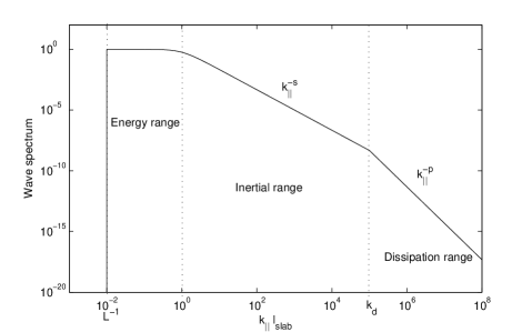
Figure 1: The power spectrum used for our calculations. We used a general spectrum with energy, inertial, and dissipation range. The dissipation wavenumber $k_{d}$ divides the inertial range from the dissipation range.

Furthermore, we used the slab bendover scale $l_{slab}$, the dissipation wavenumber $k_{d}$, the turbulence strength $\delta B_{slab}^{2}$, the inertial range spectral index $s=2\nu$ and the dissipation range spectral index $p$. The parameter $k_{min}=L^{-1}$ indicates the smallest wavenumber. Also the dynamical correlation function $\Gamma^{slab}(k_{\parallel},t)$ has to be determined which is done in the next subsection.

2.2 Improved form of the slab correlation time scale

In the past several models have been developed to approximate the dynamical correlation function $\Gamma^{slab}(k_{\parallel},t)$ (e.g. Schlickeiser & Achatz 1993, Bieber et al. 1994, Shalchi et al. 2006). Some examples are given in Table 1.

Table 1: Previous models for the slab dynamical correlation function. Here $v_{A}$ is the Alfvén velocity, $\alpha$ is a parameter which allows to adjust the strength of dynamical effects, and $\beta=\alpha Z/l_{2D}$ is used in the NADT (nonlinear anisotropic dynamical turbulence)-model ($Z=\sqrt{2}\delta B_{2D}/\sqrt{4\pi\rho_{d}}=\sqrt{2}v_{A}\delta B_{2D}/B_{0}$).

Model	$\Gamma(\vec{k},t)$
Magnetostatic model	$1$
Damping model of dynamical turbulence	$e^{-\alpha v_{A}\mid k\mid t}$
Random sweeping model	$e^{-(\alpha v_{A}kt)^{2}}$
Plasma wave model for shear Alfvén waves	$e^{\pm iv_{A}k_{\parallel}t}$
NADT-model	$e^{\pm iv_{A}k_{\parallel}t}e^{-\beta t}$

As in the most previous models we assume an exponential decorrelation of the magnetic fluctuations and, therefore

$$\Gamma^{slab}(k_{\parallel},t)=e^{i\omega t-\gamma_{c}t}.$$ (11)

In a recent article (Lazarian & Beresnyak 2006) is was shown that for slab modes

$$t_{c}^{-1}=\gamma_{c}=v_{A}\sqrt{k_{\parallel}/L}$$ (12)

and therefore

$$\Gamma^{slab}(k_{\parallel},t)=e^{-v_{A}\sqrt{k_{\parallel}/L}\cdot t}\cdot e^{i\omega\cdot t}$$ (13)

with the Alfvén speed $v_{A}$, the plasma box size $L$, and with the plasma wave dispersion relation of shear Alfvén waves

$$\omega=jv_{A}k_{\parallel}.$$ (14)

The form of Eq. (12) can be justified by the following argument (for a more detailed explanation see Lazarian & Beresnyak 2006): consider a wavepacket of Alfvén waves that moves nearly parallel to the magnetic field with the dispersion of angles $\delta k_{\perp}/k_{\parallel}\sim\Theta_{k}$. The individual waves follow the local direction of the magnetic field lines. As a result, the dispersion in angles of the wave packet cannot be less than the dispersion of angles due to the ambient Alfvén turbulence, $\Theta_{k}>\Theta_{bk}$. The latter for the Goldreich-Sridhar (1995) model

$$k_{\parallel}\sim k_{\perp}^{2/3}L_{A}^{-1/3},\quad\delta v\sim v_{A}(k_{\perp}L_{A})^{1/3}$$ (15)

is $\Theta_{bk}\sim\delta B_{k}/B_{0}\sim(k_{\perp}L)^{-1/3}$. The modes with minimal $\Theta_{k}$ are the fastest growing ones. As we establish below (see Eq. (16)) they are the least damped. Therefore for our simplified treatment we shall limit our attention to the wavepackets with resonant $k_{\parallel}^{-1}\sim r_{p}$ and $\Theta_{bk}\sim\Theta_{k}$. One can determine the characteristic perpendicular wavenumber $k_{\perp}\sim\delta k_{\perp}\sim r_{p}^{-1}(r_{p}/L)^{1/4}$ of the most parallel modes that are created by streaming CR’s. The strong Alfvénic turbulence decorrelates the wavepacket with $k_{\perp}$ on the time scale $v_{\perp}k_{\perp}$. Thus using the above expression for $k_{\perp}$ and Eq. (15) we get

$$t_{c}^{-1}=\gamma_{c}\sim-k_{\perp}v_{\perp}\sim-v_{A}k_{\perp}^{2/3}L^{-1/3}\sim-v_{A}r_{p}^{-1/2}L^{-1/2}$$ (16)

and thus Eq. (12), which, up to the ”-” that we used to denote the damping nature of the process, coincides with the damping rate obtained in Farmer & Goldreich (2004) and with the results of the numerical simulations shown in Lazarian & Beresnyak (2006, Fig. 1 therein).

The parameter $j$ is used to track the wave direction ($j=+1$ is used for forward and $j=-1$ for backward to the ambient magnetic field propagating Alfvén waves). A lot of studies have addressed the direction of propagation of Alfvénic turbulence, see for instance Bavassano (2003). In general one would expect that closer to the Sun the most waves should propagate forward and far away from the Sun the wave intensities should be equal for both directions. In the current paper we are interested in turbulence parameters at 1 AU. Thus, we simply assume that all waves propagate forward and we therefore set $j=+1$.

In the following we employ the dynamical correlation function defined by Eqs. (13) and (14) to determine the parallel mean free path within the quasilinear approach.

3 The quasilinear parallel mean free path

In the current paper we employ quasilinear theory (QLT, Jokipii 1966) to calculate the parallel mean free path. QLT can be seen as a first order perturbation theory in the small parameter $\delta B/B_{0}$. Whereas it was shown previously (e. g. Michalek & Ostrowski 1996) that QLT is accurate even if $\delta B\approx B_{0}$ if we assume slab geometry and a wave spectrum without dissipation range, it was realized by more recent test particle simulations that for non-slab models and for steep wave spectra nonlinear effects are important and QLT is no longer accurate (see e.g. Qin et al. 2006 and Shalchi 2007). In the current article we only investigate the slab model and we can therefore assume validity of QLT as it is shown in Shalchi et al. (2005) that the unphysical contribution of large scale motions arising in QLT due to its inability to account for the conservation of adiabatic invariant is small. According to Jokipii (1966), Hasselmann & Wibberenz (1968), Earl (1974), and Shalchi (2006), the parallel mean free path results from the pitch-angle-cosine average of the inverse pitch-angle Fokker-Planck coefficient $D_{\mu\mu}$ as

$$\lambda_{\parallel}={3v\over 8}\int_{-1}^{+1}d\mu\;{(1-\mu^{2})^{2}\over D_{\mu\mu}(\mu)}.$$ (17)

The pitch-angle-cosine $\mu$ is defined as $\mu=v_{\parallel}/v$. According to Teufel & Schlickeiser (2002, Eq. 25) the pitch-angle Fokker-Planck coefficient can be written as

$$D_{\mu\mu}^{i}(\mu) = {\Omega^{2}(1-\mu^{2})\over 2B_{0}^{2}}\sum_{n=-\infty}^{+\infty}\int d^{3}k\;R_{n}^{i}(\vec{k})$$ (18)

$$\left[J_{n+1}^{2}\left({k_{\perp}v_{\perp}\over\Omega}\right)P_{RR}^{i}(\vec{k})\right.$$

$$+ \left.J_{n-1}^{2}\left({k_{\perp}v_{\perp}\over\Omega}\right)P_{LL}^{i}(\vec{k})\right.$$

$$- J_{n+1}\left({k_{\perp}v_{\perp}\over\Omega}\right)J_{n-1}\left({k_{\perp}v_{\perp}\over\Omega}\right)$$

$$\times \left.\left(P_{RL}^{i}(\vec{k})e^{+2i\Psi}+P_{LR}^{i}(\vec{k})e^{-2i\Psi}\right)\right]$$

if we use helical coordinates

$$\delta B_{L} = {1\over\sqrt{2}}\left(\delta B_{x}+i\delta B_{y}\right),$$

$$\delta B_{R} = {1\over\sqrt{2}}\left(\delta B_{x}-i\delta B_{y}\right)$$ (19)

and if we neglect electric fields . In Eq. (18) we used the resonance function

$$R_{n}^{i}(\vec{k})=Re\int_{0}^{\infty}dt\;e^{-i(k_{\parallel}v_{\parallel}+n\Omega)t}\cdot\Gamma^{i}(\vec{k},t)$$ (20)

where the index $i$ stands for the different turbulence models. For pure slab geometry we have according to Teufel & Schlickeiser (2002, Eq. 33)

$$P_{RR}(\vec{k}) = P_{LL}(\vec{k})=g^{slab}(k_{\parallel}){\delta(k_{\perp})\over k_{\perp}},$$

$$P_{RL}(\vec{k}) = P_{LR}(\vec{k})=0$$ (21)

if we assume vanishing magnetic helicity. For the pitch-angle Fokker-Planck coefficient we then find

$$D_{\mu\mu}^{slab} = {\pi\Omega^{2}(1-\mu^{2})\over B_{0}^{2}}\int_{-\infty}^{+\infty}dk_{\parallel}\;g^{slab}\left(k_{\parallel}\right)$$ (22)

$$\times \sum_{n=\pm 1}R_{n}^{slab}(k_{\parallel}).$$

The resonance function for pure slab turbulence has the form

$$R_{n}^{slab}(k_{\parallel})=Re\int_{0}^{\infty}dt\;e^{-i(k_{\parallel}v_{\parallel}+n\Omega)t}\cdot\Gamma^{slab}(k_{\parallel},t).$$ (23)

With Eq. (13) for $\Gamma^{slab}(k_{\parallel},t)$, the integral in Eq. (23) is elementary and we obtain

$$R_{n}^{slab}={v_{A}\sqrt{k_{\parallel}/L}\over v_{A}^{2}k_{\parallel}/L+(k_{\parallel}v_{\parallel}+n\Omega-v_{A}k_{\parallel})^{2}}.$$ (24)

With this Breit-Wigner-type resonance function the slab Fokker-Planck coefficient can be written as

$$D_{\mu\mu}^{slab} = {2\pi\Omega^{2}(1-\mu^{2})\over B_{0}^{2}}\int_{0}^{\infty}dk_{\parallel}\;g^{slab}(k_{\parallel})$$ (25)

$$\times \sum_{n=\pm 1}{v_{A}\sqrt{k_{\parallel}/L}\over v_{A}^{2}k_{\parallel}/L+(k_{\parallel}v_{\parallel}+n\Omega-v_{A}k_{\parallel})^{2}}.$$

With the integral transformation $x=l_{slab}k_{\parallel}$ and with the parameters $R=R_{L}/l_{slab}=v/(\Omega l_{slab})$ and $\epsilon=v_{A}/v$ we obtain

$$D_{\mu\mu}^{slab} = {2\pi(1-\mu^{2})\over B_{0}^{2}l_{slab}}\int_{0}^{\infty}dx\;g^{slab}\left(k_{\parallel}={x\over l_{slab}}\right)$$ (26)

$$\times \sum_{n=\pm 1}{v_{A}\sqrt{k_{\parallel}/L}\over(v_{A}\sqrt{k_{\parallel}/L}/\Omega)^{2}+\left[xR(\mu-\epsilon)+n\right]^{2}}.$$

The slab spectrum of Eq. (9) can be written as

$$g^{slab}(x)={C(\nu)\over 2\pi}l_{slab}\delta B_{slab}^{2}\;h^{slab}(x,x_{min},\nu,\xi,p)$$ (27)

with

$$h^{slab}(x,x_{min},\nu,\xi,p)$$ (31)

$$= \left\{\begin{array}[]{ccc}0&\textnormal{for}&0\leq x<x_{min}\\ (1+x^{2})^{-\nu}&\textnormal{for}&x_{min}\leq x<\xi\\ (1+\xi^{2})^{-\nu}({\xi\over x})^{p}&\textnormal{for}&\xi\leq x\end{array}\right.$$

where we used $\xi=l_{slab}k_{d}$. Then we find for the dimensionless Fokker-Planck coefficient $\tilde{D}_{\mu\mu}^{slab}=D_{\mu\mu}^{slab}l_{slab}/v$

$$\tilde{D}_{\mu\mu}^{slab}={C(\nu)(1-\mu^{2})\over R}{\delta B_{slab}^{2}\over B_{0}^{2}}$$ (32)

$$\times \int_{0}^{\infty}dx\;h^{slab}(x,x_{min},\nu,\xi,p)$$

$$\times \sum_{n=\pm 1}{v_{A}\sqrt{x/(l_{slab}L)}/\Omega\over(v_{A}\sqrt{x/(l_{slab}L)}/\Omega)^{2}+\left[xR(\mu-\epsilon)+n\right]^{2}}.$$

By using

$${v_{A}\over\Omega}\sqrt{x\over l_{slab}L}={v_{A}\over v}{v\over\Omega l_{slab}}\sqrt{x{l_{slab}\over L}}=\epsilon R\sqrt{x\eta}$$ (33)

we finally find

$$\tilde{D}_{\mu\mu}^{slab} = {C(\nu)(1-\mu^{2})\over R}{\delta B_{slab}^{2}\over B_{0}^{2}}$$ (34)

$$\times \int_{0}^{\infty}dx\;h^{slab}(x,x_{min},\nu,\xi,p)$$

$$\times \sum_{n=\pm 1}{\epsilon R\sqrt{x\eta}\over(\epsilon R\sqrt{x\eta})^{2}+\left[xR(\mu-\epsilon)+n\right]^{2}}.$$

In Eqs. (27) - (34) we used $\rho=l_{slab}/l_{2D}$ and $x_{min}\equiv\eta=l_{slab}/L$. A numerical investigation of the integral of Eq. (34) is presented in the next section.

4 Numerical results for pitch-angle and parallel diffusion

In this section we evaluate the formulas for pitch-angle diffusion (Eq. (34)) and for the mean free path (Eq. (17)) derived in the last sections numerically for the parameter-set of Table 2 which should be appropriate for interplanetary conditions at 1 AU heliocentric distance. All formulas depend on the parameter $\epsilon$ which can be expressed as (see Shalchi et al. 2006)

$$\epsilon={v_{A}\over v}={v_{A}\over c}{\sqrt{R_{0}^{2}+R^{2}}\over R}$$ (35)

with

$$R_{0}={1\over l_{slab}\cdot B_{0}}\cdot\left\{\begin{array}[]{ccc}0.511MV&\textnormal{for}&e^{-}\\ 938MV&\textnormal{for}&p^{+}\end{array}\right.$$ (38)

For the heliospheric parameters considered in the current paper we have for electrons $R_{0}(e^{-})\approx 9.2\cdot 10^{-5}$ and protons $R_{0}(p^{+})\approx 0.169$.

In order to determine the transport coefficients of the isotropic part of the particle distribution function, e.g. the parallel mean free path, we must restrict our calculations to $\epsilon=v_{A}/v\ll 1$ (see Schlickeiser 2002 for a detailed explanation). Thus, we can only consider rigidities which satisfy the following condition:

$$R\gg{R_{0}\over\sqrt{\left(c/v_{A}\right)^{2}-1}}\approx R_{0}{v_{A}\over c}$$ (39)

For $v_{A}=33.5\;km/s$ we find for electrons the restriction $R(e^{-})\gg 10^{-8}$ and for protons $R(p^{+})\gg 2\cdot 10^{-5}$.

Table 2: Parameters used for our numerical calculations. The values should be appropriate for the solar wind at 1 AU heliocentric distance. If a parameter is different from the values below we note this separately in the corresponding figures and discussions. These values correspond to the values used in Shalchi et al. (2006).

Parameter	Symbol	Value
Inertial range spectral index	$2\nu$	$5/3$
Dissipation range spectral index	$p$	$3$
Alfvén speed	$v_{A}$	$33.5\;km/s$
Slab bendover scale	$l_{slab}$	$0.030\;AU$
Slab dissipation wavenumber	$k_{slab}$	$3\cdot 10^{6}\;(AU)^{-1}$
Mean field	$B_{0}$	$4.12\;nT$
Turbulence strength	$\delta B_{slab}/B_{0}$	$1$

4.1 The pitch-angle Fokker-Planck coefficient $D_{\mu\mu}$

Fig. 2 shows the (dimensionless) pitch-angle Fokker-Planck coefficient $\tilde{D}_{\mu\mu}=D_{\mu\mu}l_{slab}/v$ as a function of the pitch-angle-cosine $\mu$. For the rigidity we assumed $R=10^{-4}$. In this case the parameter $\epsilon$ (see Eq. (35)) is approximately $\epsilon\approx 0.2$. It seems that the minimum of the pitch-angle Fokker-Planck coefficient for protons can be found at $\mu\approx\epsilon$.

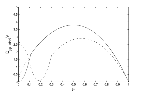
Figure 2: The pitch-angle Fokker-Planck coefficient for protons (dashed line) and electrons (solid line). Also the magnetostatic dissipationless model is shown (dotted line). Visualized is a linear plot of the dimensionless pitch-angle Fokker-Planck coefficient $\tilde{D}_{\mu\mu}$ as a function of the pitch-angle cosine $\mu$. All results are for pure slab geometry and for small rigidities $R=10^{-4}$.

In general the pitch-angle Fokker-Planck coefficient is no longer equal to zero at $90^{o}$ ($\mu=0$) as in the magnetostatic model, so that we no longer obtain an infinitely large parallel mean free path as in magnetostatic models. It should be noted, however, that QLT itself is questionable close to $90^{o}$. By considering Fig. 2 we find that at least for protons pitch-angle scattering close to $90^{o}$ is very strong due to the dynamical effects. Therefore one could assume that nonlinear effects which also lead to nonvanishing pitch-angle scattering at $90^{o}$ could be neglected.

4.2 The parallel mean free paths $\lambda_{\parallel}$

Here we present theoretical results for the parallel mean free path. We compare our results with the Palmer consensus (Palmer 1982) and pickup ion observations (Gloeckler et al. 1995, Möbius et al. 1998). In Fig. 3 we show the parallel mean free path in comparison with observations. We computed the parallel mean free paths for two different values of the smallest wave number $x_{min}$, namely for $x_{min}=0.1$ and $x_{min}=0.01$.

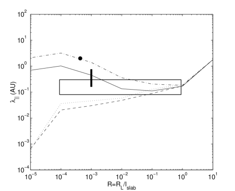
Figure 3: The quasilinear parallel mean free path $\lambda_{\parallel}$ for $x_{min}=\eta=0.1$ for electrons (solid line) and protons (dashed line), and for $x_{min}=\eta=0.01$ for electrons (dash-dotted line) and protons (dotted line) in comparison with different solar wind observations: Palmer consensus (Palmer 1982, box), Ulysses observations (Gloeckler et al. 1995, dot), AMPTE spacecraft observations (Möbius et al. 1998, vertical line).

In addition to the Palmer (1982) results we compare our results also with pickup ion observations:

1. Gloeckler et al. (1995) concluded from Ulysses observations that the parallel mean free paths of pickup protons is 2 AU at 2.4 MV rigidity (they stated conservatively that $\lambda_{\parallel}$ is of order 1 AU but actually they obtained the best fit for 2 AU). It should be noted that this observation was at high heliographic latitudes, and at a heliocentric distance of 2.34 AU; these differences should be remembered when comparing with observations at Earth orbit.

2. Möbius et al. (1998) concluded from AMPTE (Active Magnetospheric Particle Tracer Explorers) spacecraft observations that the parallel mean free paths of pickup helium ranges from 0.16 to 0.76 AU at 5.6 MV rigidity in the data they analyzed.

Both results are also illustrated in Fig. 3. As shown we can reproduce the observations theoretically.

In Fig. 4 we compare our new theoretical results with the results obtained by Shalchi et al. (2006) by applying the NADT-model in combination with the slab/2D model for the turbulence geometry.

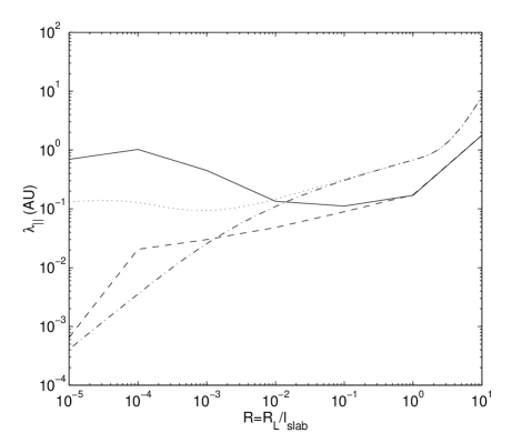
Figure 4: The parallel mean free path $\lambda_{\parallel}$ for $x_{min}=\eta=0.1$. Shown are QLT results for electrons (solid line) and protons (dashed line) in comparison with the theoretical results obtained by Shalchi et al. (2006) by applying the NADT-model in combination with the slab/2D model for the turbulence geometry (results for electron are represented by the dotted line, and the results for protons are represented by the dash-dotted line).

As shown, for small rigidities, where dissipation effects are important, we obtain a much larger parallel mean free path for electrons. For medium rigidities where the charged particles interact resonantly with the inertial range of the spectrum, the new parallel mean free path is about a factor 5 smaller since we assumed pure slab fluctuations (in comparison to the slab/2D model used in Shalchi et al. 2006). It seems that the improved model for the slab correlation function provides a much larger electron parallel mean free path for low energetic particles.

5 Summary and Conclusion

The theoretical explanation of measured parallel mean free paths in the solar system is a fundamental problem of space science. In a recent article (Shalchi et al. 2006) it has been demonstrated the these observations can indeed be reproduced theoretically. By using recent results of turbulence theory (Lazarian & Beresnyak 2006) we further improved the dynamical correlation function which is a key input in transport theory considerations. It is demonstrated in this article that the improved slab correlation time scale (see Eq. (12)) leads to a much larger parallel mean free path (see Fig. 3). This effect is important since it was argued in several previous articles that the theoretical parallel mean free path is too small (Palmer 1982, Bieber et al. 1994) in comparison with solar wind observations.

Another problem of cosmic ray scattering theory is the importance of nonlinear effects. Whereas we have applied QLT in the current article it was argued in other papers (e.g. Shalchi et al. 2004) that nonlinear effects are important for parallel diffusion. However, these nonlinear effects are directly related to the interaction between charged particles and 2D modes. These 2D modes were neglected since we assumed pure slab fluctuations. Therefore, QLT can be applied and the results presented in this article should be valid. For non-slab models, where 2D modes are present, however, the applicability of QLT is questionable. It has to be subject of future work to explore the validity of QLT for realistic turbulence models such as dynamical turbulence models in non-slab geometry.

References

- (1) Bavassano, B., 2003, AIP Conf. Proc., 679, 377
- (2) Bieber J. W., Matthaeus W. H., Smith C. W., Wanner W., Kallenrode M.-B., Wibberenz G., 1994, ApJ, 420, 294
- (3) Bruno R., Carbone V., 2005, Living Reviews in Solar Physics, 2, 4
- (4) Cho, J. & Lazarian, A., 2005, Theoretical and Computational Fluid Dynamics, 19, 127
- (5) Denskat K. U., Neubauer F. M., 1983, vol. 2280 of NASA Conference Publication, pp. 81-91, NASA, Washington, U. S. A
- (6) Earl J. A., 1974, ApJ, 193, 231
- (7) Farmer, A. J. & Goldreich, P., 2004, The Astrophysical Journal, 604, 671
- (8) Gloeckler, G., Schwadron, N. A., Fisk, L. A. & Geiss, J., 1995, Geophysical Research Letters, 22, 2665
- (9) Goldreich, P. & Sridhar, S., 1995, The Astrophysical Journal, 438, 763
- (10) Hasselmann K., Wibberenz G., 1968, Z. Geophys. 34, 353
- (11) Jokipii J. R., 1966, ApJ, 146, 480
- (12) Lazarian A. & Beresnyak A., 2006, Monthly Notices of the Royal Astronomical Society, 373, 1195
- (13) Melrose D. B., 1968, Ap&SS, 2, 171
- (14) Michalek G., Ostrowski M., 1996, Nonlinear Processes in Geophysics, 3, 66
- (15) Möbius, E., Rucinski, D., Lee, M. A. & Isenberg, P. A., 1998, Journal of Geophysical Research, 10, 257
- (16) Palmer, I. D., 1982, Reviews of Geophysics and Space Physics, 20, 335
- (17) Qin, G., Matthaeus, W. H. & Bieber, J. W., 2006, The Astrophysical Journal, 640, L103
- (18) Schlickeiser R., Cosmic Ray Astrophysics, Springer-Verlag, Berlin, 2002
- (19) Schlickeiser, R. & Achatz, U., 1993, Journal of Plasma Physics, 49, 63
- (20) Shalchi, A., Bieber, J. W., Matthaeus, W. H. & Qin, G., 2004, The Astrophysical Journal, 616, 617
- (21) Shalchi, A., Yan, H. & Lazarian, A., 2005, Monthly Notices of the Royal Astronomical Society, 356, 1064
- (22) Shalchi A., Bieber J. W., Matthaeus W. H., Schlickeiser R., 2006, ApJ, 642, 230
- (23) Shalchi A., 2006, A&A, 448, 809
- (24) Shalchi A., 2007, Journal of Physics G: Nuclear and Particle Physics, 34, 209
- (25) Teufel A., Schlickeiser R., 2002, A&A, 393, 703
- (26) Yan, H. & Lazarian, A., 2002, Physical Review Letters, 89, 28