Statistics of conductance and shot-noise power for chaotic cavities

Abstract

We report on an analytical study of the statistics of conductance, $g$, and shot-noise power, $p$, for a chaotic cavity with arbitrary numbers $N_{1,2}$ of channels in two leads and symmetry parameter $\beta=1,2,4$. With the theory of Selberg’s integral the first four cumulants of $g$ and first two cumulants of $p$ are calculated explicitly. We give analytical expressions for the conductance and shot-noise distributions and determine their exact asymptotics near the edges up to linear order in distances from the edges. For $0<g<1$ a power law for the conductance distribution is exact. All results are also consistent with numerical simulations.
       PACS numbers: 73.23.-b, 73.50.Td, 05.45.Mt, 73.63.Kv

1 Introduction

Our goal is to discuss the statistics of conductance and shot-noise power for chaotic cavities using essentially the properties of Selberg’s integral. The static conductance $G$ relates linearly the time averaged current $\overline{I(t_{0})}=G\cdot V$ to the external voltage $V$ between two electron reservoirs. Fluctuations of the current around its mean value are conventionally described by the spectral noise power $P=2\int_{0}^{\infty}dt\overline{\delta I(t+t_{0})\delta I(t_{0})}$, with $\delta I=I-\overline{I}$. As temperature goes to zero, the only source of noise that remains non-vanishing is related to the discreteness of the electric charge carriers, the so-called shot-noise. For mesoscopic conductors, an adequate framework for the problematic is based on random-matrix-theory (RMT) approach to quantum transport, we refer to [1, 2] for reviews.

We consider a chaotic cavity with two attached leads supporting $N_{1}$ and $N_{2}$ channels, respectively, and coupled perfectly to the interior of the cavity. According to the Landauer-Büttiker formalism, the conductance $G$ and the shot-noise power $P$ can be expressed in terms of the transmission eigenvalues $T_{i}$ as follows:

$$G=G_{0}\sum_{i=1}^{n}T_{i}\equiv G_{0}\cdot g$$ (1)

and

$$P=P_{0}\sum_{i=1}^{n}T_{i}(1-T_{i})\equiv P_{0}\cdot p\,,$$ (2)

where $G_{0}=\frac{2e^{2}}{h}$ is the conductance quantum and $P_{0}=2eVG_{0}$. The positive numbers $T_{i}\leq 1$ are the $n\equiv\mathrm{min}(N_{1},N_{2})$ non-zero eigenvalues of the matrix $tt^{\dagger}$, with the transmission matrix $t$ being the $N_{1}\times N_{2}$ submatrix of the full scattering matrix and consisting of transition amplitudes from $N_{1}$ left to $N_{2}$ right channels. For chaotic cavities, universal fluctuations of $T_{i}$ can be described by RMT [1].

Considering the moments of $g$ and $p$, the exact (RMT) results valid at arbitrary channel numbers $N_{1,2}$ and repulsion parameter $\beta$ were reported in the literature only for the average and variance of the conductance [3, 4, 1]:

$$\langle g\rangle=\frac{N_{1}N_{2}}{N-1+\frac{2}{\beta}}\,,\qquad N\equiv N_{1}+N_{2}\,,$$ (3)

$$\mbox{var}(g)=\frac{2}{\beta}\frac{N_{1}N_{2}(N_{1}-1+\frac{2}{\beta})(N_{2}-1+\frac{2}{\beta})}{(N-2+\frac{2}{\beta})(N-1+\frac{2}{\beta})^{2}(N-1+\frac{4}{\beta})}\,,$$ (4)

and very recently for the average shot-noise power [5]:

$$\langle p\rangle=\frac{N_{1}N_{2}(N_{1}-1+\frac{2}{\beta})(N_{2}-1+\frac{2}{\beta})}{(N-2+\frac{2}{\beta})(N-1+\frac{2}{\beta})(N-1+\frac{4}{\beta})}=N_{1}N_{2}\frac{\beta}{2}\frac{\mathrm{var}(g)}{\langle g\rangle}\,.$$ (5)

To derive these results in a uniform way, it is convenient to use the known expression for the joint probability density of transmission eigenvalues $T_{i}$ [5, 1]

$$\mathcal{P}(T_{1},T_{2},\ldots,T_{n})=\mathcal{N}_{\beta}^{-1}\prod_{i=1}^{n}T_{i}^{\alpha-1}\prod_{j<k}|T_{j}-T_{k}|^{\beta}\,,\quad\alpha\equiv\frac{\beta}{2}(|N_{1}-N_{2}|+1)\,,$$ (6)

to perform the corresponding integrations on Eqs. (1)–(2). The normalization constant $\mathcal{N}_{\beta}$ above is given by

$$\mathcal{N}_{\beta}=\prod_{j=1}^{n-1}\frac{\Gamma(1+\frac{\beta}{2}(1+j))\;\Gamma(\alpha+\frac{\beta}{2}j)\;\Gamma(1+\frac{\beta}{2}j)}{\Gamma(1+\frac{\beta}{2})\;\Gamma(1+\alpha+\frac{\beta}{2}(n+j-1))}$$ (7)

and assures that (6) is a probability density. It is known for discrete positive $n$ and continuous $\alpha$ and $\beta$ as Selberg’s integral [6].

As to the distribution functions, simple closed expressions can be obtained for the conductance distribution at $n=1,2$ [3, 4, 7] and for the shot-noise distribution at $N_{1}=N_{2}=1$ only [8]. To the best of our knowledge, no general results valid at arbitrary $N_{1,2}$ and $\beta$ have been presented thus far.

2 Cumulants

To study the cumulants of $g$ and $p$, one needs to know what are the moments $\langle T_{1}^{n_{1}}\cdots T_{k}^{n_{k}}\rangle$, with $\langle\ldots\rangle$ standing for the integration over the joint probability density (6) and $n_{i}\geqslant 0$. Moments with all $n_{i}=1$ as well as $\langle T_{1}^{2}\rangle$ can be found from recursion relations already given in Mehta’s book [6] that come from the Selberg’s integral theory. The latter can be successfully applied [5] to derive results (3)–(5). This approach was recently extended further to find $\langle T_{1}^{3}\rangle$ and $\langle T_{1}(1-T_{1})T_{2}(1-T_{2})\rangle$ exactly [9]. Here, we have calculated all moments with $\sum_{i}n_{i}\leqslant 4$ by using tricks of partial integrations to reduce all moments to forms of Selberg’s integral. We will report on that in more detail elsewhere [10]. By this method we are able to calculate the so-called skewness (third cumulant) of the conductance, which we represent in the following compact form:

$$\langle\langle g^{3}\rangle\rangle \equiv \langle(g-\langle g\rangle)^{3}\rangle$$ (8)

$$= \mathrm{var}(g)\frac{4[(1-\frac{2}{\beta})^{2}-(N_{1}-N_{2})^{2}]}{\beta(N-3+\frac{2}{\beta})(N-1+\frac{2}{\beta})(N-1+\frac{6}{\beta})}\,.$$

It is worth noting that the skewness vanishes for symmetric cavities ($N_{1}=N_{2}$) at $\beta=2$. This also holds for any odd cumulant of the conductance, as the conductance distribution becomes symmetric around $\frac{n}{2}$ in this case.

We have also calculated the kurtosis $\langle\langle g^{4}\rangle\rangle$ of the conductance (which is the fourth cumulant of $g$) and the variance $\langle\langle p^{2}\rangle\rangle=\mathrm{var}(p)$ of the shot-noise power (the second cumulant). These expressions are given explicitly but are too lengthy to be reported here. In the case of the single-mode leads, $N_{1}=N_{2}=1$, one gets $\langle\langle g^{4}\rangle\rangle=-\frac{32}{4725},-\frac{1}{120},-\frac{1}{540}$ and $\mathrm{var}(p)=\frac{4}{525},\frac{1}{180},\frac{1}{180}$ at the values of $\beta=1$, 2, 4, respectively. In the opposite semiclassical limit of large channel numbers, $N_{1,2}\gg 1$, we write the results as the following $1/N$ expansions:

$$\frac{\langle\langle g^{4}\rangle\rangle}{\mathrm{var}(g)} = \frac{24}{\beta^{2}N^{6}}\Bigl{[}(N_{1}-N_{2})^{2}(N_{1}^{2}+N_{2}^{2}-4N_{1}N_{2})$$ (9)

$$+\frac{\beta-2}{\beta N}\Bigl{(}12(N_{1}^{4}+N_{2}^{4})-64N_{1}N_{2}(N_{1}^{2}+N_{2}^{2})+105N_{1}^{2}N_{2}^{2}\Bigr{)}\Bigr{]}$$

$$+{\cal O}(1/N^{4})\,,$$

$$\frac{\mathrm{var}(p)}{\langle p\rangle} = \frac{2}{\beta N^{5}}\Bigl{[}N_{1}^{4}+N_{2}^{4}-4N_{1}N_{2}(N_{1}-N_{2})^{2}$$ (10)

$$+\frac{\beta-2}{\beta N}\Bigl{(}9(N_{1}^{4}+N_{2}^{4})-42N_{1}N_{2}(N_{1}^{2}+N_{2}^{2})+70N_{1}^{2}N_{1}^{2}\Bigr{)}\Bigr{]}$$

$$+{\cal O}(1/N^{3})\,.$$

One can readily see that higher cumulants contribute at least in the next order of $\frac{1}{N}$, so that the full distributions get more Gaussian-like as $N$ grows. This tendency becomes even stronger for the conductance distribution in symmetric cavities at $\beta=2$, as $\langle\langle g^{4}\rangle\rangle$ vanishes then in the leading and next-to-leading orders. In this case of symmetric cavities, $N_{1,2}=n\gg 1$, we can further find:

$$\langle\langle g^{4}\rangle\rangle = \frac{3}{128\beta^{3}n^{3}}\biggl{(}1-\frac{2}{\beta}+\frac{(\beta+2)^{2}}{2\beta^{2}n}\biggr{)}+\mathcal{O}\Bigl{(}\frac{1}{n^{5}}\Bigr{)}\,,$$ (11)

$$\mathrm{var}(p) = \frac{1}{64\beta}\biggl{(}1+\frac{\beta-2}{\beta n}+\frac{4+\beta(\beta-2)}{2\beta^{2}n^{2}}\biggr{)}+\mathcal{O}\Bigl{(}\frac{1}{n^{3}}\Bigr{)}\,.$$ (12)

3 Distributions

Finally, we discuss shortly the distribution of the conductance, $P_{g}(g)=\langle\delta(g-\sum_{i}T_{i})\rangle$ and that of the shot-noise power, $P_{p}(p)=\langle\delta(p-\sum_{i}T_{i}(1-T_{i})\rangle$, deferring a detailed consideration to a separate publication [11]. Writing the functions $P_{g}(g)$ and $P_{p}(p)$ as Fourier series over the interval of support, we obtain, e.g., for the conductance distribution the following representation:

$$P_{g}^{(\beta)}(g)=n!\sum_{m=1}^{\infty}\frac{2}{n}\sin\bigl{(}\frac{m\pi g}{n}\bigl{)}A^{(\beta)}(m)$$ (13)

where $A^{(\beta)}(m)$ is known at $\beta=1,2,4$. For example,

$$A^{(2)}(m)=C_{2}\mbox{\,Im\,}\det B^{(2)}_{kl}(m)$$ (14)

is given by the imaginary part of the determinant of the following matrix:

$$B^{(2)}_{kl}(m)=\int_{0}^{1}dT\;T^{\alpha+k+l-3}{\rm e}^{im\pi T/n},\qquad\mbox{for}\quad k,l=1,2,\ldots,n\;.$$ (15)

In a similar way we may write $P_{g}^{(1)}(g)$ and $P_{g}^{(4)}(g)$ as imaginary parts of certain Pfaffians. The sum (13) can be done numerically where care has to be taken for the Pfaffians, which may equivalently be written as quaternion determinants of certain self-dual antisymmetric matrices, which are easier to be calculated.

Analogous expressions are also obtained for $P_{p}^{(\beta)}(p)$.

Figure 1: The conductance distribution at $\beta=1$, $N_{1}=4$ and $N_{2}=1$, 2, 3, 4, 5, 7, 9 (from left to right).

It is worth noting that at any finite $n$ these distributions are continuous but not analytic functions everywhere. Nonanalyticity in the distribution of conductances in quasi-one-dimensional wires (the cusp point at $g=1$) was recently reported in [7, 12], see also [3]. In the present context of chaotic cavities, it can be understood from the following geometrical consideration. In the case of $P_{g}(g)$, calculating the average amounts to an integration over an ($n-1$)–dimensional plane $g=\sum_{i}T_{i}$ cut by the $n$–dimensional cube $0\leqslant T_{i}\leqslant 1$, such that there appear (sometimes weak) singularities at all points $g=M$ with an integer $M$, $0\leqslant M\leqslant n$. A similar situation appears also for $P_{p}(p)$. Here, we integrate over the ($n-1$)–dimensional sphere $\frac{n}{4}-p=\sum_{i}(T_{i}-\frac{1}{2})^{2}$ and singularities appear whenever the sphere touches one edge or surface of the cube, that is for $p=\frac{M}{4}$ with $0\leqslant M\leqslant n$.

Figure 1 illustrates the conductance distribution at $\beta=1$ keeping $N_{1}=4$ fixed and varying $N_{2}$ from 1 to 9. In figure 2, we plot the distribution of the shot-noise power at $\beta=2$, keeping $N_{1}=4$ fixed and varying $N_{2}$ from 2 to 14. In both cases one can see the tendency of the distributions to get peaked around the mean values, so that in the bulk they can be effectively described by a Gaussian with the known mean and variance, see Eqs. (3) – (5) and (10).

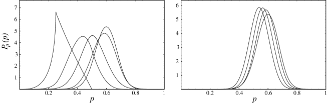
Figure 2: Distributions of the shot-noise power at $\beta=2$, $N_{1}=4$ and $N_{2}=2$, 3, 4, 6, 8 (left plot) and at $\beta=2$, $N_{1}=4$ and $N_{2}=8$, 10, 12, 14 (right plot).

4 Asymptotics

We are able to give some exact asymptotics near the edges of support of the distributions expressed in terms of exact integrals, which are related to some general forms of Selberg’s integral. For example, for $0<g<1$ we find

$$P_{g}^{(\beta)}(g)=\mathrm{const}\times g^{\alpha n+\frac{\beta}{2}n(n-1)-1}\,,$$ (16)

where the proportionality factor is exactly known. This result follows easily from calculating the powers of $g$ in $\langle\delta(g-\sum_{i}T_{i})\rangle$ under scaling of all $T_{i}\to g\widetilde{T}_{i}$ and noticing that the upper integration limit of $\widetilde{T}_{i}$ remains unchanged ($=1$) as long as $g<1$. Similarly, $P_{g}^{(\beta)}(g)$ behaves near the upper edge as follows:

$$P_{g}^{(\beta)}(g)\propto(n-g)^{(n-1)(1+\frac{\beta}{2}n)}\,,\qquad n-1<g<n\,.$$ (17)

For the distribution of the shot-noise power, one finds

$$P_{p}^{(\beta)}(p)\propto\left(\frac{n}{4}-p\right)^{\frac{n}{2}(1+\frac{\beta}{2}(n-1))-1}\,,\qquad\frac{n-1}{4}<p<\frac{n}{4}\,,$$ (18)

whereas near the lower edge ($0<p<\frac{1}{4}$) the asymptotics is a bit more complicated, since the contribution of the corners of the cube of integration become disconnected. These expressions can be extended outside the regions specified above, being valid then in a linear order in distances from the edges. The expansions can even be improved and all constants can be given explicitly as expressions containing products of Gamma functions from Selberg’s integral.

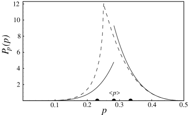
Figure 3: The distribution of the shot-noise power (dashed line) and corresponding asymptotics (full lines) at $\beta=4$ and $N_{1}=4$, $N_{2}=2$.

In figure 3, we show as an example the distribution of the shot-noise power at $\beta=4$, $N_{1}=4$, $N_{2}=2$ (dashed line) with calculated asymptotics near the edges (full lines). Indicated as dots are the average $\langle p\rangle$ and $\langle p\rangle\pm\sqrt{\mathrm{var}(p)}$ known exactly. We have also compared (and found a perfect agreement) all the expressions with numerical simulations of the RMT statistics of $T_{i}$ and resulting distributions for $g$ and $p$.

5 Conclusions

In summary, we have applied essentially the theory of Selberg’s integral to the problems of quantum transport in chaotic cavities. The cumulants up to the forth order for the conductance and up to the second order for the shot-noise power have been calculated exactly at arbitrary channel numbers and repulsion parameter $\beta$. We have also given the conductance and shot-noise distributions in closed form suitable for subsequent analytic analysis (e.g., finding asymptotics) as well as for numerical implementations. It would be desirable to compare our findings with relevant experimental results, e.g., in microwave cavities which became available recently [13]. This could, however, be not so straightforward, as it requires taking into account effects of dephasing [14] and absorption [15] as well. Further work in this direction is needed.

Support by SFB/TR12 of the DFG is acknowledged with thanks.

References

• [1] C.Β W.Β J. Beenakker, Rev. Mod. Phys. 69, 731 (1997).
• [2] Ya.Β M. Blanter and M. BΓΌttiker, Phys. Rep. 336, 1 (2000).
• [3] H.Β U. Baranger and P.Β A. Mello, Phys. Rev. Lett. 73, 142 (1994).
• [4] R.Β A. Jalabert, J.-L. Pichard, and C.Β W.Β J. Beenakker, Europhys. Lett. 27, 255 (1994).
• [5] D.Β V. Savin and H.-J. Sommers, Phys. Rev. B 73, 081307 (2006).
• [6] M.Β L. Mehta, Random Matrices, 2nd ed. (Academic Press, New York, 1991).
• [7] A. GarcΓ­a-MartΓ­n and J.Β J. SΓ‘enz, Phys. Rev. Lett. 87, 116603 (2001).
• [8] M.Β H. Pedersen, S.Β A. van Langen, and M.Β BΓΌttiker, Phys. Rev. B 57, 1838 (1998).
• [9] M. Novaes, Phys. Rev. B 75, 073304 (2007).
• [10] D.Β V. Savin, H.-J. Sommers and W. Wieczorek, in preparation
• [11] W. Wieczorek, D.Β V. Savin and H.-J. Sommers, in preparation
• [12] K.Β A. Muttalib, P. WΓΆlfle, A. GarcΓ­a-MartΓ­n and V.Β A. Gopar, Europhys. Lett. 61, 95 (2003).
• [13] S. Hemmady, J. Hart, X. Zheng, T.Β M. Antonsen, E. Ott and S.Β M. Anlage, Phys. Rev. B 74, 195326 (2006).
• [14] P. W. Brouwer and C. W. J. Beenakker, Phys. Rev. B 55, 4695 (1997).
• [15] Y. V. Fyodorov, D. V. Savin, H.-J. Sommers, J. Phys. A 38, 10731 (2005).