We study the $q$-deformed Knizhnik-Zamolodchikov equation in path representations of the Temperley-Lieb algebras. We consider two types of open boundary conditions, and in both cases we derive factorised expressions for the solutions of the qKZ equation in terms of Baxterised Demazurre-Lusztig operators. These expressions are alternative to known integral solutions for tensor product representations. The factorised expressions reveal the algebraic structure within the qKZ equation, and effectively reduce it to a set of truncation conditions on a single scalar function. The factorised expressions allow for an efficient computation of the full solution once this single scalar function is known. We further study particular polynomial solutions for which certain additional factorised expressions give weighted sums over components of the solution. In the homogeneous limit, we formulate positivity conjectures in the spirit of Di Francesco and Zinn-Justin. We further conjecture relations between weighted sums and individual components of the solutions for larger system sizes.

Factorised solutions of Temperley-Lieb $q$KZ equations on a segment

1. Introduction

The $q$-deformed Knizhnik-Zamolodchikov equations (qKZ) are widely recognized as important tools in the computation of form factors in integrable quantum field theories [44] and correlation functions in conformal field theory and solvable lattice models [26]. They can be derived using the representation theory of affine quantum groups [24] or, equivalently and using a dual setup, from the affine and double affine Hecke algebra [5]. The qKZ equations have been extensively studied in tensor product modules of affine quantum groups or Hecke algebras, and much is known about their solutions in the case of cyclic boundary conditions [47, 46]. We refer to [22] and references therein for extensive literature on the qKZ equations.

Recently interest has arisen in the qKZ equation in the context of the Razumov-Stroganov conjectures. These relate the integrable spin-1/2 quantum XXZ spin chain [45, 39] in condensed matter physics and the O(1) loop model [2, 40] in statistical mechanics, to alternating sign matrices and plane partitions [4]. Further developments surrounding the Razumov-Stroganov conjectures include progress on loop models [6, 33, 15, 19, 20, 51, 18] and quantum XXZ spin chains [7, 37, 38], the stochastic raise and peel models [9, 10, 35, 36, 1], lattice supersymmetry [3, 23, 48, 49], higher spin and higher rank cases [50, 17, 41], as well as connections to the Brauer algebra and (multi)degrees of certain algebraic varieties [8, 16, 31].

The connection to the qKZ equation was realised by Pasquier [34] and Di Francesco and Zinn-Justin [17], by generalising the Razumov-Stroganov conjectures to include an extra parameter $q$ or $\tau=-(q+q^{-1})$. In particular, the polynomial solutions for level one qKZ equations display intriguing positivity properties and are conjectured to be related to weighted plane partitions and alternating sign matrices [34, 17, 28, 13, 18].

In the Razumov-Stroganov context one considers the qKZ equation in a path representation for $SL(k)$ quotients of the Hecke algebra, using cyclic as well as open (non-affine) boundary conditions. In the case $k=2$ this quotient corresponds to the Temperley-Lieb algebra, for which there is a well known and simple equivalence between the path representation and its graphical loop, or link pattern, representation. In this paper we study the qKZ equation for $k=2$ in the path representation and for the two types of open boundary conditions also considered in [13, 51, 18].

The solution of the qKZ equation is a function in $N$ variables $x_{i}$ $i=1,\ldots,N$ taking values in the path representation. The components of this vector valued function can be expressed in a single scalar function which we call the base function. We derive factorised expressions for the components of the solution of the qKZ equations for the Temperley-Lieb algebra (referred to as type A) and the one-boundary Temperley-Lieb algebra (type B) with arbitrary parameters. The factorised expressions are given in terms of Baxterised Demazurre-Lusztig operators, acting on the base function which we assume to be known. The formula for type A was already derived for Kazhdan-Lusztig elements of Grasmannians by Kirillov and Lascoux [30]. We further reduce the qKZ equation to a set of truncation relations that determine the base function. These relations also appear in a factorised form. We conjecture that the truncation relations can be recast entirely in terms of Baxterised elements of the symmetric group.

Restricting to polynomial solutions, the factorised expressions provide an efficient way for computing explicit solutions. We note here that polynomial solutions may also be obtained from Macdonald polynomials [5, 34, 28, 29]. Using the factorised expressions, we compute explicit polynomial solutions of the level one qKZ equations, recovering and extending the results of Di Francesco [14] in the case of type A, and of Zinn-Justin [51] in the case of type B. We would like to emphasize the importance of such explicit solutions as a basis for experimentation and discovery of novel results. Based on the explicit solutions, and in analogy with Di Francesco [13, 14] and Kasatani and Pasquier [28], we formulate new positivity conjectures in the case of type B for two-variable polynomials in the homogeneous limit ($x_{i}\rightarrow 0$) of the solutions of the qKZ equations. In the inhomogeneous case, the factorised expressions furthermore suggest to define linear combinations (weighted partial sums) of the components of the solution in a very natural way. Special cases of these partial sums are also considered in the homogeneous limit by Razumov, Stroganov and Zinn-Justin [37, 38] and by Di Francesco and Zinn-Justin [18]. We conjecture identities between the partial sums and individual components of solutions for larger system sizes.

The first three sections of this paper are a review of known results. We define the Hecke and Temperley-Lieb algebras of type A and B, the path representations and explain the qKZ equation in these representations. In Section 4 we state our main theorems concerning factorised solutions and truncation conditions for the qKZ equation of type A and B. These results are proved in Section 6 and Appendix A. The fifth section contains a list of conjectures regarding the explicit polynomial solutions of the qKZ equation. These conjectures relate to the positivity of solutions in the homogeneous limit, and to natural partial sums over components of the solution. Our observations are based on explicit solutions for type A and B which are listed in Appendices B and C.

Throughout the following we will use the notation $[x]_{q}$ for the usual q-number

$$[x]_{q}=\frac{q^{x}-q^{-x}}{q-q^{-1}}.$$

The notation $[x]$ will always refer to base $q$.

Acknowledgments

Our warm thanks go to Arun Ram, Ole Warnaar and Keiichi Shigechi for useful discussions. JdG thanks the Australian Research Council for financial assistance. PP was supported by RFBR grant No. 05-01-01086-a and by the DFG-RFBR grant (436 RUS 113/909/0- 1(R) and 07-02-91561-a)

2. Relevant algebras and their representations

2.1. Iwahori-Hecke algebras

2.1.1. Type A

Definition 1.

The Iwahori-Hecke algebra of type $A_{N}$, denoted by $\mathcal{H}_{N}^{\rm A}(q)$, is the unital algebra defined in terms of generators $g_{i}$, $i=1,\ldots,N-1$, and relations

$$(g_{i}-q)(g_{i}+q^{-1})=0,\qquad g_{i}g_{j}=g_{j}g_{i}\quad\forall\,i,j:\,|i-j|>1,$$

$$g_{i}g_{i+1}g_{i}=g_{i+1}g_{i}g_{i+1}.$$ (2.1)

Hereafter we always assume

$$q\in{\mathbb{C}}\setminus\{0\},\quad\mbox{ and}\quad[k]\neq 0\quad\forall\,k=2,3,\dots,N,$$ (2.2)

in which case the algebra $\mathcal{H}_{N}^{\rm A}(q)$ is semisimple. It is isomorphic to the group algebra of the symmetric group ${\mathbb{C}}[S_{N}]\simeq\mathcal{H}_{N}^{\rm A}(1)$.

It is sometimes convenient to use two other presentations of the algebra $\mathcal{H}_{N}^{\rm A}(q)$ in terms of the elements $a_{i}$ and $s_{i}$

$$a_{i}:=q-g_{i},\qquad s_{i}:=q^{-1}+g_{i}\,,\qquad i=1,\dots,N-1.$$

For each particular value of index $i$ the elements $a_{i}$ and $s_{i}$ are mutually orthogonal unnormalised projectors

$$a_{i}s_{i}=s_{i}a_{i}=0,\qquad a_{i}+s_{i}=[2]\,,$$

generating the subalgebra ${\mathcal{H}}^{\rm A}_{2}(q)\hookrightarrow{\mathcal{H}}^{\rm A}_{N}(q)$. Traditionally they are called the antisymmetrizer and the symmetrizer and associated, respectively, with the two possible partitions of the number 2: $\{1^{2}\}$ and $\{2\}$.

The $\mathcal{H}^{\rm A}_{N}(q)$ defining relations (2.1) in terms of generators $a_{i}$, $i=1,\ldots,N-1$, read

$$a_{i}^{2}=[2]\,a_{i},\qquad a_{i}a_{j}=a_{j}a_{i}\quad\forall\,i,j:\,|i-j|>1,$$

$$a_{i}a_{i+1}a_{i}-a_{i}=a_{i+1}a_{i}a_{i+1}-a_{i+1},$$ (2.3)

and in terms of $s_{i}$, $i=1,\ldots,N-1$, they read

$$s_{i}^{2}=[2]\,s_{i},\qquad s_{i}s_{j}=s_{j}s_{i}\quad\forall\,i,j:\,|i-j|>1,$$

$$s_{i}s_{i+1}s_{i}-s_{i}=s_{i+1}s_{i}s_{i+1}-s_{i+1}.$$

2.1.2. Type B

Definition 2.

The Iwahori-Hecke algebra of type $B_{N}$, denoted by $\mathcal{H}^{\rm B}_{N}(q,\omega)$, is the unital algebra defined in terms of generators $g_{i}$, $i=0,\ldots,N-1$, satisfying, besides (2.1), relations

$$(g_{0}+q^{\omega})(g_{0}+q^{-\omega})=0,\qquad g_{0}g_{i}=g_{i}g_{0}\quad\forall\,i>1,$$

$$g_{0}g_{1}g_{0}g_{1}=g_{1}g_{0}g_{1}g_{0}.$$ (2.4)

If in addition to (2.2) we assume $[\omega\pm k]\neq 0\;\;\forall\,k\in 0,1,\dots,N-1,$ then the algebra $\mathcal{H}^{\rm B}_{N}(q,w)$ becomes semisimple. Hereafter we do not need the semisimplicity and we only assume that $[\omega+1]\neq 0$.

It is sometimes convenient to use the presentations of $\mathcal{H}^{\rm B}_{N}(q,\omega)$ in terms of either the antisymmetrizers $a_{i}$, or the symmetrizers $s_{i}$, supplemented, respectively, by the boundary generators

$$a_{0}:=\frac{-q^{-\omega}-g_{0}}{q^{\omega+1}-q^{-\omega-1}},\qquad\mbox{or}\qquad s_{0}:=\frac{q^{\omega}+g_{0}}{q^{\omega+1}-q^{-\omega-1}}.$$ (2.5)

The generators $a_{0}$ and $s_{0}$ are mutually orthogonal unnormalised projectors,

$$a_{0}s_{0}=s_{0}a_{0}=0,\qquad a_{0}+s_{0}=\frac{[\omega]}{[\omega+1]}.$$

The defining relations (2.4) written in terms $a_{0}$ and $a_{i}$ read

$$a_{0}^{2}=\frac{[\omega]}{[\omega+1]}a_{0},\qquad a_{0}a_{i}=a_{i}a_{0}\quad\forall\,i>1,$$

$$a_{0}a_{1}a_{0}a_{1}-a_{0}a_{1}=a_{1}a_{0}a_{1}a_{0}-a_{1}a_{0},$$ (2.6)

and written in terms of $s_{0}$ and $s_{i}$ they read

$$s_{0}^{2}=\frac{[\omega]}{[\omega+1]}s_{0},\qquad s_{0}s_{i}=s_{i}s_{0}\quad\forall\,i>1,$$

$$s_{0}s_{1}s_{0}s_{1}-s_{0}s_{1}=s_{1}s_{0}s_{1}s_{0}-s_{1}s_{0}.$$

2.2. Baxterised elements and their graphical presentation

It is well known that the defining relations of the Iwahori-Hecke algebras (2.1), (2.4) can be generalised to include a so-called spectral parameter (see [27, 25] and references therein). This generalisation is sometimes called Baxterisation and is relevant both in the representation theory of these algebras as well as in their applications to the theory of integrable systems.

2.2.1. Type A

For the algebra $\mathcal{H}_{N}^{\rm A}(q)$, the Baxterised elements $g_{i}(u)$, $i=1,\dots,N-1,$ are defined as

$$g_{i}(u):=\,q^{-2u}\,\frac{g_{i}-q^{2u-1}}{g_{i}-q^{-2u-1}},$$

which we can write alternatively as

$$g_{i}(u)=\,\frac{q^{u}-[u]\,g_{i}}{[u+1]}\,=\,\frac{[1-u]+[u]\,a_{i}}{[1+u]}\,=\,1-\frac{[u]}{[u+1]}s_{i}.$$ (2.7)

Here $u\in{\mathbb{C}}\setminus\{-1\}$ is the spectral parameter. It can be shown that the following relations hold

$$g_{i}(u)g_{i}(-u)=1,\qquad\forall\,u\in{\mathbb{C}}\setminus\{-1,1\},$$ (2.8)

$$g_{i}(u)g_{i+1}(u+v)g_{i}(v)=g_{i+1}(v)g_{i}(u+v)g_{i+1}(u),$$ (2.9)

$$g_{i}(u)g_{j}(v)=g_{j}(v)g_{i}(u)\quad\forall\,i,j:\,|i-j|>1,$$ (2.10)

The relations (2.7)–(2.10) are equivalent to the defining set of conditions (2.1). The relations (2.8) and (2.9) are called, respectively, the unitarity condition and the Yang-Baxter equation.

Notice that the unitarity condition is not valid at the degenerate points $u=\pm 1$. It is therefore useful in certain cases to use a different normalisation for the Baxterised elements,

$$h_{i}(u):=\,\frac{[1-u]}{[u]}g_{i}(-u)\,=\,\frac{[u+1]}{[u]}-a_{i}\,=\,s_{i}-\frac{[u-1]}{[u]}.$$ (2.11)

Note that now the elements $h_{i}(u)$ are ill-defined at $u=0$. In this normalisation we have

$$h_{i}(u)h_{i}(-u)=1-\frac{1}{[u]^{2}},\qquad h_{i}(1)=s_{i},\qquad h_{i}(-1)=-a_{i},$$

and $h_{i}(u)$ still satisfies the Yang-Baxter and the commutativity equations (2.9) and (2.10). We also note that $h_{i}$ satisfies the simple but very useful identity

$$h_{i}(u)=h_{i}(v)+\frac{[v-u]}{[u][v]}.$$ (2.12)

2.2.2. Type B

In this case we additionally define

$$g_{0}(u):=\,q^{-2u}\frac{[\tfrac{\omega+\nu}{2}+u](g_{0}+q^{2u-\nu})}{[\tfrac{\omega+\nu}{2}-u](g_{0}+q^{-2u-\nu})},$$

which alternatively can be written as

$$g_{0}(u)=\,\frac{k(u,\nu)-[2u][\omega+1]a_{0}}{k(-u,\nu)}=\,1+\frac{[2u][\omega+1]}{k(-u,\nu)}s_{0},$$ (2.13)

where $k(u,\nu):=[\tfrac{\omega+\nu}{2}+u][\tfrac{\omega-\nu}{2}+u]$, and $\nu$ is an additional arbitrary parameter.

The boundary Baxterised element $g_{0}(u)$ satisfies relations

$$g_{0}(u)g_{0}(-u) =1,$$ (2.14)

$$g_{0}(v)g_{1}(u+v)g_{0}(u)g_{1}(u-v) =g_{1}(u-v)g_{0}(u)g_{1}(u+v)g_{0}(v),$$ (2.15)

$$g_{0}(u)g_{i}(v) =g_{i}(v)g_{0}(u)\quad\forall\,i>1,$$

which are equivalent to the defining relations (2.4). Relations (2.14) and (2.15) are called, respectively, the unitarity condition and the reflection equation [42]. An alternative normalisation for the boundary Baxterised element is

$$h_{0}(u):=\,-\frac{k(u/2,\nu)}{[u][\omega+1]}g_{0}(-u/2)\,=\,-\frac{k(-u/2,\nu)}{[u][\omega+1]}-a_{0}\,=\,s_{0}-\frac{k(u/2,\nu)}{[u][\omega+1]}.$$ (2.16)

In this normalisation we find

$$h_{0}(\omega\pm\nu)\,=\,-a_{0}, \qquad h_{0}(-\omega\pm\nu)\,=\,s_{0},$$

$$h_{0}(v-u)h_{1}(v)h_{0}(u+v)h_{1}(u)\, =\,h_{1}(u)h_{0}(u+v)h_{1}(v)h_{0}(v-u).$$ (2.17)

2.2.3. Graphical presentation

For our purposes it is convenient to represent the Baxterised elements graphically as tiles and the boundary Baxterised element as a half-tile

$$\begin{picture}(0.0,30.0)(0.0,21.0)\qbezier[25](43.0,0.0)(43.0,25.0)(43.0,50.0)\qbezier[5](58.0,40.0)(58.0,45.0)(58.0,50.0)\qbezier[25](73.0,0.0)(73.0,25.0)(73.0,50.0)\qbezier[6](159.0,0.0)(159.0,6.0)(159.0,12.0)\qbezier[5](159.0,40.0)(159.0,45.0)(159.0,50.0)\qbezier[25](174.0,0.0)(174.0,25.0)(174.0,50.0)\put(34.0,-10.0){$\scriptstyle i-\mathit{1}$} \put(70.0,-10.0){$\scriptstyle i+\mathit{1}$} \put(157.0,-11.0){$\scriptstyle\mathit{0}$} \put(172.0,-11.0){$\scriptstyle\mathit{1}$} \end{picture}g_{i}(u)=\ \raisebox{-32.0pt}{\includegraphics[height=50.0pt]{Rmatrix.eps}}\ ,\quad\qquad g_{0}(u)=\ \raisebox{-14.0pt}{\includegraphics[height=34.0pt]{Kmatrix.eps}}\ .$$

The (half-)tiles are placed on labeled vertical lines and they can move freely along the lines unless they meet other (half-)tiles. Multiplication in the algebra corresponds to a simultaneous placement of several (half-)tiles on the same picture and a rightwards order of terms in the product corresponds to a downwards order of (half-)tiles on the picture. In this way, the Yang-Baxter equation (2.9) can be depicted as

$$\raisebox{-40.0pt}{\includegraphics[height=80.0pt]{ybe.eps}}\;\;\;=\;\;\;\raisebox{-40.0pt}{\includegraphics[height=80.0pt]{ybe2.eps}}\ .$$ (2.18)

and the reflection equation can be depicted as

$$\begin{picture}(0.0,0.0)\qbezier[10](0.0,-45.0)(0.0,-32.5)(0.0,-20.0)\qbezier[2](16.0,-45.0)(16.0,-42.5)(16.0,-40.0)\qbezier[2](70.0,-45.0)(70.0,-42.5)(70.0,-40.0)\qbezier[8](86.0,-45.0)(86.0,-35.0)(86.0,-25.0)\put(-3.0,-55.0){$\scriptstyle\mathit{0}$} \put(13.0,-55.0){$\scriptstyle\mathit{1}$} \put(67.0,-55.0){$\scriptstyle\mathit{0}$} \put(83.0,-55.0){$\scriptstyle\mathit{1}$} \end{picture}\raisebox{-40.0pt}{\includegraphics[height=80.0pt]{reflection.eps}}\quad=\quad\raisebox{-40.0pt}{\includegraphics[height=80.0pt]{reflection2.eps}}\ .$$

For the alternative set of Baxterised elements we will use dashed pictures,

$$\phantom{a}\begin{picture}(0.0,30.0)(0.0,21.0)\qbezier[4](61.0,0.0)(61.0,4.0)(61.0,8.0)\qbezier[6](159.0,0.0)(159.0,6.0)(159.0,12.0){ \put(159.0,10.0){\qbezier[10](0.0,0.0)(0.0,1.5)(0.0,3.0)}\put(159.0,18.0){\qbezier[10](0.0,0.0)(0.0,1.5)(0.0,3.0)}\put(159.0,26.0){\qbezier[10](0.0,0.0)(0.0,1.5)(0.0,3.0)}\put(159.0,34.0){\qbezier[10](0.0,0.0)(0.0,1.5)(0.0,3.0)} \put(159.0,10.0){\qbezier[10](0.0,0.0)(1.0,1.0)(2.0,2.0)}\put(165.0,16.0){\qbezier[10](0.0,0.0)(1.0,1.0)(2.0,2.0)}\put(171.0,22.0){\qbezier[10](0.0,0.0)(1.0,1.0)(2.0,2.0)} \put(159.0,39.0){\qbezier[10](0.0,0.0)(1.0,-1.0)(2.0,-2.0)}\put(165.0,33.0){\qbezier[10](0.0,0.0)(1.0,-1.0)(2.0,-2.0)}\put(171.0,27.0){\qbezier[10](0.0,0.0)(1.0,-1.0)(2.0,-2.0)} } \put(58.0,-11.0){$\scriptstyle i$} \put(157.0,-11.0){$\scriptstyle\mathit{0}$} \put(162.0,22.0){$u$} \end{picture}h_{i}(u)=\ \raisebox{-15.0pt}{\includegraphics[height=36.0pt]{hi.eps}}\,,\qquad\quad h_{0}(u)=\ \vspace{20pt}$$ (2.19)

The picture of the Yang-Baxter equation for the dashed tiles is the same as (2.18), but the picture of the reflection equation (2.17) has a different arrangement of the spectral parameters

(2.20)

Let us remark that expressions for the boundary half-tile $g_{0}(u)$ and the dashed half-tile $h_{0}(u)$ depend on an arbitrary parameter $\nu$ which is not shown in the pictures. For the dashed half-tile we shall exploit this degree of freedom in Section 4.2, see (4.4).

2.3. Temperley-Lieb algebras

The Iwahori-Hecke algebras have a well known series of $SL(2)$ type, or Temperley-Lieb, quotients whose irreducible representations are classified in the semisimple case by partitions into one or two parts (i.e., by the Young diagrams containing at most two rows). The Temperley-Lieb algebra can be described in terms of equivalence classes of the generators $a_{i}$ (different generators belong to different equivalence classes). Below we use the notation $e_{i}$ for the equivalence class of $-a_{i}$.

Definition 3.

The Temperley-Lieb algebra of type $A_{N}$, denoted by $\mathcal{T}^{\rm A}_{N}(q)$, is the unital algebra defined in terms of generators $e_{i}$, $i=1,\ldots,N-1,\,$ satisfying the relations

$$e_{i}^{2}=-[2]e_{i},\quad e_{i}e_{j}=e_{j}e_{i}\quad\forall\,i,j:\,|i-j|>1,$$

$$e_{i}e_{i\pm 1}e_{i}=e_{i}.$$ (2.21)

Definition 4.

The Temperley-Lieb algebra of type $B_{N}$, $\mathcal{T}^{\rm B}_{N}(q,\omega)$ (also called the blob algebra [32]), is the unital algebra defined in terms of generators $e_{i}$, $i=0,\ldots,N-1,\,$ satisfying, besides (2.21), the relations

$$e_{0}^{2}=-\frac{[\omega]}{[\omega+1]}e_{0},\quad e_{0}e_{i}=e_{i}e_{0}\quad\forall\,i>1,$$

$$e_{1}e_{0}e_{1}=e_{1}.$$ (2.22)

2.3.1. Graphical presentation

We reserve empty tiles and half-tiles for the generators $e_{i}$ and $e_{0}$

$$\begin{picture}(0.0,10.0)(16.0,25.0)\qbezier[4](61.0,0.0)(61.0,4.0)(61.0,8.0)\qbezier[6](158.0,0.0)(158.0,6.0)(158.0,12.0)\put(58.0,-11.0){$\scriptstyle i$} \put(157.0,-11.0){$\scriptstyle\mathit{0}$} \end{picture}e_{i}=\ \raisebox{-18.0pt}{\includegraphics[height=36.0pt]{ei.eps}}\,,\qquad\qquad e_{0}=\ \raisebox{-18.0pt}{\includegraphics[height=36.0pt]{e0.eps}}\,.\vspace{23pt}$$ (2.23)

The defining relations (2.21) and (2.22) are depicted, respectively, as

$$-\frac{1}{[2]}$$   =        =        =  , (2.24)

and

                   $$=\;-\frac{[\omega]}{[\omega+1]}$$ ,          =      .      (2.25)

2.3.2. Baxterisation

Obviously, one can adapt all formulas for the Baxterised elements from the previous subsection to the case of Temperley-Lieb algebras by the substitution $a_{i}\mapsto-e_{i}$. We shall follow tradition and will use a special notation — $R_{i}(u)$ and $K_{0}(u)$ — for the Baxterised elements and the boundary Baxterised element of the Temperley-Lieb algebras. In the same normalisation used for $g_{i}(u)$ (see (2.7), (2.13)), we have

$$R_{i}(u) :=\,\frac{[1-u]-[u]\,e_{i}}{[1+u]}\,,$$

$$K_{0}(u) :=\,\frac{k(u,\delta)+[2u][\omega+1]e_{0}}{k(-u,\delta)},\quad k(u,\delta):=[\tfrac{\omega+\delta}{2}+u][\tfrac{\omega-\delta}{2}+u].$$ (2.26)

Here we have intentionally used a different notation to denote an arbitrary additional parameter, $\delta$ instead of $\nu$ which was used in the Iwahori-Hecke case, see (2.13). The two parameters $\delta$ and $\nu$ will play different roles in what follows below (see the comment after (3.12)).

The elements $R_{i}(u)$ and $K_{0}(u)$ satisfy the unitarity conditions (2.8), (2.14), the Yang-Baxter equation (2.9) and the reflection equation (2.15). They are usually called the R-matrix and the reflection matrix. This notation comes from the theory of integrable quantum spin chains. The path representations of the Temperley-Lieb algebras, which are introduced in the next subsection and which are used later on in the qKZ equations, are invariant subspaces of the state space of certain quantum spin-1/2 XXZ chains, see, e.g., [7].

Remark 1.

In order to make contact with other notations in the literature, we note that our notation here correspond to those in [7] if we identify $q={\rm e}^{{\rm i}\gamma}$, $q^{\omega}\rightarrow{\rm e}^{{\rm i}\omega}$, $q^{\delta}\rightarrow-{\rm e}^{{\rm i}\delta}$, and in [51] to $q^{\delta}=-\zeta$. Further useful notations in [7] that we shall employ later are:

$$\tau=-[2],\qquad\tau^{\prime}=\sqrt{2+[2]}=[2]_{q^{1/2}}\ ,\qquad a=-\frac{[\omega+1]}{[\frac{\omega-\delta}{2}][\frac{\omega+\delta}{2}]}.$$

2.4. Representations on paths

We will now decribe an important and well-known representation of the Temperley-Lieb algebras of type A and type B on Dyck and Ballot paths respectively.

2.4.1. Dyck path representation

Definition 5.

A Dyck path $\alpha$ of length $N$ is a vector of $\,(N+1)\,$ local integer heights

$$\alpha=(\alpha_{0},\alpha_{1},\ldots,\alpha_{N}),$$

such that $\alpha_{0}=0$, $\alpha_{N}=0$ for $N$ even and $\alpha_{N}=1$ for $N$ odd, and the heights are subject to the constraints $\alpha_{i}\geq 0$ and $\alpha_{i+1}-\alpha_{i}=\pm 1$.

By $\mathcal{D}_{N}$ we denote the set of all Dyck paths of length $N$.

Each Dyck path $\alpha$ of length $N$ corresponds uniquely to a word in $w_{\alpha}\in\mathcal{T}^{\rm A}_{N}(q)$, represented pictorially as

$$\begin{picture}(0.0,20.0) \put(101.0,1.0){\line(0,-1){23.0}} \put(235.0,1.0){\line(0,-1){23.0}} \put(97.0,-14.5){\put(5.0,15.0){\line(1,0){5.0}}}\put(107.5,-14.5){\put(5.0,15.0){\line(1,0){5.0}}}\put(118.0,-14.5){\put(5.0,15.0){\line(1,0){5.0}}}\put(128.5,-14.5){\put(5.0,15.0){\line(1,0){5.0}}}\put(139.0,-14.5){\put(5.0,15.0){\line(1,0){5.0}}}\put(149.5,-14.5){\put(5.0,15.0){\line(1,0){5.0}}}\put(160.0,-14.5){\put(5.0,15.0){\line(1,0){5.0}}}\put(170.5,-14.5){\put(5.0,15.0){\line(1,0){5.0}}}\put(181.0,-14.5){\put(5.0,15.0){\line(1,0){5.0}}}\put(191.5,-14.5){\put(5.0,15.0){\line(1,0){5.0}}}\put(202.0,-14.5){\put(5.0,15.0){\line(1,0){5.0}}}\put(212.5,-14.5){\put(5.0,15.0){\line(1,0){5.0}}}\put(223.0,-14.5){\put(5.0,15.0){\line(1,0){5.0}}} \end{picture}\mbox{N even:}\qquad w_{\alpha} = \raisebox{-33.0pt}{\includegraphics[height=80.0pt]{word2dyck.eps}}\;,$$

,

where the empty tiles at horizontal position $i$ are the generators $e_{i}$, see (2.23).

We now define an action of the algebra $\mathcal{T}^{\rm A}_{N}(q)$ on a space which is spanned linearly by states $|\alpha\rangle$ labeled by the Dyck paths, identifying the states $|\alpha\rangle$ with the corresponding words $w_{\alpha}\in\mathcal{T}^{\rm A}_{N}(q)$. This action is given by a set of elementary transformations of pictures shown in (2.24). A typical example of such an action is given in Figure 1.

Figure 1. The result of $e_{i}|\alpha\rangle$ if $\alpha$ has a slope at $i$. If $i+r$ is the first position to the right of an upward slope at $i$ whose height is equal to that at $i$, i.e. $\alpha_{i+r}=\alpha_{i}>0$, then a layer of tiles between $i$ and $i+r$ is peeled off the original path and the result is again a Dyck path. A similar peeling mechanism to the left works for downward slopes.

In doing so we find the following representation of the algebra $\mathcal{T}^{\rm A}_{N}(q)$:

Proposition 1.

The action of $e_{i}$ for $i=1,\ldots,N-1$ on Dyck paths is explicitly given by

$$\bullet\$$ Local Minimum:

$$e_{i}|\ldots,\alpha_{i}+1,\alpha_{i},\alpha_{i}+1,\ldots\rangle=|\ldots,\alpha_{i}+1,\alpha_{i}+2,\alpha_{i}+1,\ldots\rangle,$$

$$\bullet\$$ Local Maximum:

$$e_{i}|\ldots,\alpha_{i}-1,\alpha_{i},\alpha_{i}-1,\ldots\rangle=-[2]\ |\ldots,\alpha_{i}-1,\alpha_{i},\alpha_{i}-1,\ldots\rangle,$$

$$\bullet\ \alpha_{i-1}<\alpha_{i}<\alpha_{i+1}$$ Uphill Slope: .

Let $$j>i \alpha_{j}=\alpha_{i} \alpha_{l}>\alpha_{i}\;\;\forall\,l:\;i<l<j$$ be such that and , then

$$e_{i}|\ldots,\alpha_{i}-1,\alpha_{i},\alpha_{i}+1,\alpha_{i+2},\ldots,\alpha_{j},\ldots\rangle=$$

$$\hphantom{\text{Uphill Slope:}}|\ldots,\alpha_{i}-1,\alpha_{i},\alpha_{i}-1,\alpha_{i+2}-2,\ldots,\alpha_{j-1}-2,\alpha_{j},\alpha_{j+1},\ldots\rangle,$$

$$\bullet\ \alpha_{i-1}>\alpha_{i}>\alpha_{i+1}$$ Downhill Slope: .

Let $$k<i \alpha_{k}=\alpha_{i} \alpha_{l}>\alpha_{i}\;\;\forall\,l:\;k<l<i$$ be such that and , then

$$e_{i}|\ldots,\alpha_{k},\ldots,\alpha_{i-2},\alpha_{i}+1,\alpha_{i},\alpha_{i}-1,\ldots\rangle=$$

$$\hphantom{\text{Uphill Slope:}}|\ldots,\alpha_{k},\alpha_{k+1}-2,\ldots,\alpha_{i-2}-2,\alpha_{i}-1,\alpha_{i},\alpha_{i}-1,\ldots\rangle$$

Remark 2.

For generic values of $q$ the Dyck path representation is the irreducible representation of the Temperley-Lieb algebra $\mathcal{T}^{\rm A}_{N}(q)$ corresponding in the conventional classification to the partition $\{\lfloor\tfrac{N+1}{2}\rfloor,\lfloor\tfrac{N}{2}\rfloor\}$.

Definition 6.

We call the unique Dyck path without local minima in the bulk the maximal Dyck path and denote it $\Omega^{\rm A}$. Explicitly this path reads:

$$\Omega^{\rm A}=(0,1,2,\dots,\lfloor\tfrac{N-1}{2}\rfloor,\lfloor\tfrac{N+1}{2}\rfloor,\lfloor\tfrac{N-1}{2}\rfloor,\dots,\epsilon_{N}),$$

where $\epsilon_{N}:=N\bmod 2$ is the parity of $N$.

It is clear from Proposition 1 that the maximal Dyck path plays a role of a highest weight element of the Dyck path representation.

2.4.2. Ballot path representation

Definition 7.

A Ballot path $\alpha$ of length $N$ is a vector of $(N+1)$ local integer heights

$$\alpha=(\alpha_{0},\alpha_{1},\ldots,\alpha_{N}),$$

such that $\alpha_{i}\geq 0$, $\alpha_{i+1}-\alpha_{i}=\pm 1$ and $\alpha_{N}=0$.

We denote the set of all Ballot paths of the length $N$ by $\mathcal{B}_{N}$ .

Each Ballot path $\alpha$ of length $N$ corresponds uniquely to a word $w_{\alpha}\in\mathcal{T}^{\rm B}_{N}(q,w)$, represented pictorially as

$$\begin{picture}(0.0,0.0) \put(131.5,-7.0){\line(0,-1){23.0}} \par\put(265.5,-7.0){\line(0,-1){23.0}} \put(127.0,-21.0){\put(5.0,15.0){\line(1,0){5.0}}}\put(137.5,-21.0){\put(5.0,15.0){\line(1,0){5.0}}}\put(148.0,-21.0){\put(5.0,15.0){\line(1,0){5.0}}}\put(158.5,-21.0){\put(5.0,15.0){\line(1,0){5.0}}}\put(169.0,-21.0){\put(5.0,15.0){\line(1,0){5.0}}}\put(179.5,-21.0){\put(5.0,15.0){\line(1,0){5.0}}}\put(190.0,-21.0){\put(5.0,15.0){\line(1,0){5.0}}}\put(200.5,-21.0){\put(5.0,15.0){\line(1,0){5.0}}}\put(211.0,-21.0){\put(5.0,15.0){\line(1,0){5.0}}}\put(221.5,-21.0){\put(5.0,15.0){\line(1,0){5.0}}}\put(232.0,-21.0){\put(5.0,15.0){\line(1,0){5.0}}}\put(242.5,-21.0){\put(5.0,15.0){\line(1,0){5.0}}}\put(253.0,-21.0){\put(5.0,15.0){\line(1,0){5.0}}} \put(131.5,-6.0){\line(-1,0){15.0}} \put(131.5,38.0){\line(-1,0){15.0}} \put(118.5,13.0){\vector(0,1){25.0}} \put(118.5,19.0){\vector(0,-1){25.0}} \put(95.0,14.0){$\scriptstyle\alpha_{0}=\mathit{4}$} \end{picture}\mbox{N even:}\qquad w_{\alpha} = \hskip 30.0pt\raisebox{-40.0pt}{\includegraphics[height=80.0pt]{word2ballot.eps}}\;,\qquad\qquad$$

,

where the empty (half-)tiles at horizontal position $i$ ($0$) are the generators $e_{i}$ ($e_{0}$), see (2.23).

Now we can define an action of the algebra $\mathcal{T}^{\rm B}_{N}(q,\omega)$ on the space which is spanned linearly by states $|\alpha\rangle$ labeled by the Ballot paths, identifying the states $|\alpha\rangle$ with the corresponding words $w_{\alpha}\in\mathcal{T}^{\rm B}_{N}(q,\omega)$. We thus find the following representation of the algebra $\mathcal{T}^{\rm B}_{N}(q,\omega)$:

Proposition 2.

The action of $e_{i}$ for $i=1,\ldots,N-1$ on Ballot paths is explicitly given by Proposition 1 in the case of a local extremum or an uphill slope. In the remaining cases we find

$$\bullet\$$ Downhill Slope, Type I:

If there exists $$k<i \alpha_{k}=\alpha_{i} \alpha_{l}>\alpha_{i}\;\forall\,l:\,k<l<i$$ such that and , then

$$e_{i}|\ldots,\alpha_{k},\ldots,\alpha_{i-2},\alpha_{i}+1,\alpha_{i},\alpha_{i}-1,\ldots\rangle=$$

$$\hphantom{\hskip 85.35826pt}|\ldots,\alpha_{k},\alpha_{k+1}-2,\ldots,\alpha_{i-2}-2,\alpha_{i}-1,\alpha_{i},\alpha_{i}-1,\ldots\rangle$$

$$\bullet\$$ Downhill Slope, Type IIa:

If $$i \alpha_{k}>\alpha_{i}\;\forall\,k<i$$ is odd and , then

$$e_{i}|\alpha_{0},\ldots,\alpha_{i-2},\alpha_{i}+1,\alpha_{i},\alpha_{i}-1,\ldots\rangle=$$

$$\hphantom{\hskip 85.35826pt}|\alpha_{0}-2,\ldots,\alpha_{i-2}-2,\alpha_{i}-1,\alpha_{i},\alpha_{i}-1,\ldots\rangle.$$ (2.27)

$$\bullet\$$ Downhill Slope, Type IIb:

If $$i \alpha_{k}>\alpha_{i}\;\forall\,k<i$$ is even and , then

$$e_{i}|\alpha_{0},\ldots,\alpha_{i-2},\alpha_{i}+1,\alpha_{i},\alpha_{i}-1,\ldots\rangle=$$

$$\hphantom{\hskip 85.35826pt}-\frac{[\omega]}{[\omega+1]}\ |\alpha_{0}-2,\ldots,\alpha_{i-2}-2,\alpha_{i}-1,\alpha_{i},\alpha_{i}-1,\ldots\rangle.$$ (2.28)

The action of the boundary generator $e_{0}$ is given by

$$\bullet\ i=0$$ Uphill Slope at :

$$e_{0}|\alpha_{0},\alpha_{0}+1,\alpha_{2},\ldots\rangle=|\alpha_{0}+2,\alpha_{0}+1,\alpha_{2},\ldots\rangle$$

$$\bullet\ i=0$$ Downhill Slope at :

$$e_{0}|\alpha_{0},\alpha_{0}-1,\alpha_{2},\ldots\rangle=-\frac{[\omega]}{[\omega+1]}|\alpha_{0},\alpha_{0}-1,\alpha_{2},\ldots\rangle$$

Remark 3.

For generic values of $q$ and $\omega$ the Ballot path representation is the irreducible representation of the Temperley-Lieb algebra $\mathcal{T}^{\rm B}_{N}(q,\omega)$ corresponding to bi-partition $\{\lfloor\tfrac{N+1}{2}\rfloor\},\,\{\lfloor\tfrac{N}{2}\rfloor\}$.

Definition 8.

We call the unique Ballot path without local minima in the bulk the maximal Ballot path and denote it by $\Omega^{\rm B}$. Explicitly this path reads:

$$\Omega^{\rm B}=(N,N-1,\dots,2,1,0).$$

As follows from the Proposition 2 the maximal Ballot path plays a role of a highest weight element of the Ballot path representation.

3. $q$-deformed Knizhnik-Zamolodchikov equation

3.1. Definition

Let us consider a linear combination $|\Psi\rangle$ of states $|\alpha\rangle$ with coefficients $\psi_{\alpha}$ taking values in the ring of formal series in $N$ variables $q^{\pm x_{i}},\;i=1,2,\dots,N$:

$$|\Psi(x_{1},\ldots,x_{N})\rangle=\sum_{\alpha}\psi_{\alpha}(x_{1},\ldots,x_{N})|\alpha\rangle.$$

Here $\alpha$ runs over the set of either Dyck (type A), or Ballot (type B) paths of length $N$.

The qKZ equation in the Temperley-Lieb algebra setting is a system of finite difference equations on the vector $|\Psi\rangle$. Actually, we consider the qKZ equation in an alternative form with permutations in place of finite differences. This is historically the first form it appeared in literature [43]. In both types A and B the qKZ equation reads universally [51],

$$R_{i}(x_{i}-x_{i+1})|\Psi\rangle =\pi_{i}|\Psi\rangle,\qquad\forall\,i=1,\ldots,N-1,$$ (3.1)

$$K_{0}(-x_{1})|\Psi\rangle =\pi_{0}|\Psi\rangle,$$ (3.2)

$$|\Psi\rangle =\pi_{N}|\Psi\rangle.$$ (3.3)

Here $R_{i}$ are the Baxterised elements of the Temperley-Lieb algebra, $K_{0}$ is the boundary Baxterised element in the type B case and $K_{0}$ is the identity operator in type A. The operators $R_{i}(x_{i}-x_{i+1})$ and $K_{0}(-x_{1})$ act on states $|\alpha\rangle$, whereas the operators $\pi_{i}$ permute or reflect arguments of the coefficient functions

$$\pi_{i}\psi_{\alpha}(\ldots,x_{i},x_{i+1},\ldots) =\psi_{\alpha}(\ldots,x_{i+1},x_{i},\ldots),$$

$$\pi_{0}\psi_{\alpha}(x_{1},\ldots) =\psi_{\alpha}(-x_{1},\ldots),$$ (3.4)

$$\pi_{N}\psi_{\alpha}(\ldots,x_{N}) =\psi_{\alpha}(\ldots,-\lambda-x_{N}).$$ (3.5)

Here $\lambda\in{\mathbb{C}}$ is a parameter related to the level of the qKZ equation, see [22].

Remark 4.

Clearly, the elementary permutations $\pi_{i}$, $i=1,\dots,N-1,$ are the generators of the symmetric group $S_{N}$, whereas $\pi_{0}$ and $\pi_{N}$ are left and right boundary reflections. They satisfy the relations

$$\pi_{i}^{2}=1,\qquad\pi_{i}\pi_{i+1}\pi_{i}=\pi_{i+1}\pi_{i}\pi_{i+1},\qquad\qquad\qquad\qquad\;\;\pi_{i}\pi_{j}=\pi_{j}\pi_{i}\quad\forall\,i,j:|i-j|>1,$$

$$\pi_{0}^{2}=1,\qquad\pi_{0}\pi_{1}\pi_{0}\pi_{1}=\pi_{1}\pi_{0}\pi_{1}\pi_{0},\qquad\qquad\qquad\qquad\;\;\;\pi_{0}\pi_{i}=\pi_{i}\pi_{0}\quad\forall\,i>1,$$

$$\pi_{N}^{2}=1,\qquad\pi_{N}\pi_{N-1}\pi_{N}\pi_{N-1}=\pi_{N-1}\pi_{N}\pi_{N-1}\pi_{N},\qquad\pi_{N}\pi_{i}=\pi_{i}\pi_{N}\;\;\forall\,i<N-1.$$

Therefore the unitarity conditions (2.8), (2.14), the Yang-Baxter relation (2.9) and the reflection equation (2.15) for the operators $R_{i}$ and $K_{0}$ are consistency conditions for the qKZ equation.

3.2. Algebraic interpretation

In this subsection we consider the algebraic content of the qKZ equation. We follow the lines of the paper [34].

3.2.1. Type A

Consider equation (3.1). Here the R-matrix $R_{i}(x_{i}-x_{j})$ acts on the states $|\alpha\rangle$, $\alpha\in\mathcal{D}_{N}$, while the operator $\pi_{i}$ acts on the functions $\psi_{\alpha}(x_{1},\ldots,x_{N})$. In other words, the qKZ equation (3.1) written out in components becomes

$$\sum_{\alpha\in\mathcal{D}_{N}}\psi_{\alpha}(x_{1},\ldots,x_{N})\,(R_{i}(x_{i}-x_{i+1})|\alpha\rangle)=\sum_{\alpha\in\mathcal{D}_{N}}(\pi_{i}\psi_{\alpha})(x_{1},\ldots,x_{N})|\alpha\rangle,$$

which can be rewritten as

$$\sum_{\alpha\in\mathcal{D}_{N}}\psi_{\alpha}(x_{1},\ldots,x_{N})\,(-e_{i}|\alpha\rangle)\\ =\sum_{\alpha\in\mathcal{D}_{N}}\left(\frac{[x_{i}-x_{i+1}+1]}{[x_{i}-x_{i+1}]}\pi_{i}+\frac{[x_{i}-x_{i+1}-1]}{[x_{i}-x_{i+1}]}\right)\psi_{\alpha}(x_{1},\ldots,x_{N})|\alpha\rangle\\ =\sum_{\alpha\in\mathcal{D}_{N}}\left(a_{i}\psi_{\alpha}\right)(x_{1},\ldots,x_{N})|\alpha\rangle.$$ (3.6)

Here we have used notation

$$a_{i} :=\,\frac{1}{[x_{i}-x_{i+1}]}(\pi_{i}-1)[x_{i+1}-x_{i}+1]\,$$

$$\,=\,(\pi_{i}+1)\frac{[x_{i}-x_{i+1}-1]}{[x_{i}-x_{i+1}]},\qquad i=1,2,\dots,N-1,$$ (3.7)

for symmetrising operators acting on functions in the variables $x_{i}$ [21]. These operators satisfy the Hecke relations (2.1.1). Moreover, they generate a faithful representation of the algebra $\mathcal{H}_{N}^{\rm A}(q)$ in the space of functions in $N$ variables $x_{i}\;(i=1,\dots,N)$, thus justifying the use of the identical notation $a_{i}$ in (2.1.1) and in (3.2.1). The generator $g_{i}=q-a_{i}$ in this representation is known as the Demazurre-Lusztig operator [5]. The alternative set of generators $s_{i}$ and the Baxterised elements $h_{i}(u)$ (2.11) in this particular representation read

$$s_{i} =\frac{[x_{i}-x_{i+1}+1]}{[x_{i}-x_{i+1}]}\,(1-\pi_{i}),$$

$$h_{i}(u) =\frac{[x_{i}-x_{i+1}+u]}{[u][x_{i}-x_{i+1}]}\,-\,\frac{[x_{i}-x_{i+1}+1]}{[x_{i}-x_{i+1}]}\pi_{i}.$$ (3.8)

Looking back at the equations (3.6) we notice that their solution amounts to constructing an explicit homomorphism from the Dyck path representation of the Temperley-Lieb algebra $\mathcal{T}^{\rm A}_{N}(q)$ into the functional representation (3.2.1) of the Iwahori-Hecke algebra $\mathcal{H}^{\rm A}_{N}(q)$:

$$|\alpha\rangle\mapsto\psi_{\alpha}\quad\forall\alpha\in\mathcal{D}_{N},$$ (3.9)

where $\psi_{\alpha}$ are the components of the solution $|\Psi\rangle$ of the qKZ equation of type A.

3.2.2. Type B

In this case we additionally have a non-trivial operator $K_{0}$ affecting equation (3.2), which reads in components:

$$\sum_{\alpha\in\mathcal{B}_{N}}\psi_{\alpha}(x_{1},\ldots,x_{L})\,(K_{0}(-x_{1})|\alpha\rangle)=\sum_{\alpha\in\mathcal{B}_{N}}(\pi_{0}\psi_{\alpha})(x_{1},\ldots,x_{L})|\alpha\rangle,$$

where the summation is taken now over all Ballot paths. Recalling the definition

$$k(u,\delta)=[u+\frac{\omega+\delta}{2}][u+\frac{\omega-\delta}{2}],$$

from (2.26), this can be rewritten as

$$\sum_{\alpha\in\mathcal{B}_{N}}\psi_{\alpha}(x_{1},\ldots,x_{N})\,(-e_{0}|\alpha\rangle)\\ =\sum_{\alpha\in\mathcal{B}_{N}}\left(\frac{k(x_{1},\delta)}{[2x_{1}][\omega+1]}\pi_{0}-\frac{k(-x_{1},\delta)}{[2x_{1}][\omega+1]}\right)\psi_{\alpha}(x_{1},\ldots,x_{N})|\alpha\rangle\\ =\sum_{\alpha\in\mathcal{B}_{N}}\left(a_{0}\psi_{\alpha}\right)(x_{1},\ldots,x_{N})|\alpha\rangle.$$ (3.10)

where we have denoted

$$a_{0}:=-(\pi_{0}+1)\frac{k(-x_{1},\delta)}{[2x_{1}][\omega+1]}\,=\,\frac{1}{[2x_{1}][\omega+1]}(\pi_{0}-1)k(-x_{1},\delta)$$ (3.11)

The operator $a_{0}$ and the operators $a_{i}$ from (3.2.1) satisfy the defining relations (2.6) for the type B Iwahori-Hecke algebra. Moreover, the realisation (3.11), (3.2.1) gives a faithful representation of $\mathcal{H}^{B}_{N}(q,\omega)$. The generator $s_{0}$ defined in (2.5) and the boundary Baxterised element $h_{0}(u)$ from (2.16) in this realisation read

$$s_{0}=\frac{k(x_{1},\delta)}{[2x_{1}][\omega+1]}(1-\pi_{0}),\qquad h_{0}(u)=s_{0}-\frac{k(u/2,\nu)}{[u][\omega+1]}.$$ (3.12)

Let us stress here the difference between the parameters $\delta$ and $\nu$. The “physical” parameter $\delta$ appears in the definition of the boundary Baxterised element $K_{0}(u)$ and therefore enters the qKZ equation and the boundary conditions of related integrable models, see e.g. [7, 51]. The parameter $\nu$ is introduced here for the first time in this section. It plays an auxilliary role and we will fix it later to obtain a convenient presentation of the solution of the qKZ equation of type B, see (4.4) below.

Finally, the relation (3.10) states that the solution $|\Psi\rangle$ of the qKZ equation of type B encodes an explicit homomorphism from the Ballot path representation of the Temperley-Lieb algebra $\mathcal{T}^{\rm B}_{N}(q,\omega)$ into the functional representation (3.2.1), (3.11) of the Iwahori-Hecke algebra $\mathcal{H}^{\rm B}_{N}(q,\omega)$:

$$|\alpha\rangle\mapsto\psi_{\alpha}\quad\forall\,\alpha\in\mathcal{B}_{N}.$$

3.3. Preliminary analysis

3.3.1. Type A

Equation (3.6) breaks up into two cases, depending whether or not a path $\alpha$ in the sum on the right-hand side of (3.6) has a local maximum at $i$, i.e. whether or not it is of the form $\alpha=(\ldots,\alpha_{i}-1,\alpha_{i},\alpha_{i}-1,\ldots)$. We will first look at the case in which it does not.

Case i): $\alpha$ does not have a local maximum at $i$.

As each term in the left-hand side of (3.6) is of the form $e_{i}|\alpha\rangle$, and hence corresponds to a local maximum at $i$,

the coefficient of $|\alpha\rangle$ in the right-hand side of (3.6) has to equal zero. Hence we obtain

$$-(a_{i}\psi_{\alpha})(x_{1},\ldots,x_{N})\equiv(h_{i}(-1)\psi_{\alpha})(x_{1},\ldots,x_{N})=0,$$ (3.13)

which can be rewritten as

$$(\pi_{i}-1)\left\{[x_{i}-x_{i+1}-1]\psi_{\alpha}(x_{1},\ldots,x_{N})\right\}=0\quad\text{for}\;|\alpha\rangle\not\propto e_{i}|\alpha^{\prime}\rangle.$$

Hence, if $|\alpha\rangle\not\propto e_{i}|\alpha^{\prime}\rangle$ the function

$$[x_{i}-x_{i+1}-1]\psi_{\alpha}(x_{1},\ldots,x_{N})$$

is symmetric in $x_{i}$ and $x_{i+1}$ which implies that $[x_{i+1}-x_{i}-1]$ divides $\psi_{\alpha}(x_{1},\ldots,x_{N})$ and the ratio is symmetric with respect to $x_{i}$ and $x_{i+1}$.

Iterating (3.1) we find

$$\Psi(x_{1},\ldots,x_{k-1},x_{m},x_{k},\ldots,x_{m-1},x_{m+1},\ldots x_{N})=\\ R_{k}(x_{k}-x_{m})\cdots R_{m-1}(x_{m-1}-x_{m})\Psi(x_{1},\ldots,x_{N}).$$ (3.14)

Consider now the component $\psi_{\alpha}$ on the LHS of (3.14), where $\alpha$ does not have a local maximum at any $i$ for $k\leq i\leq m-1$. This component can only arise from the same component on the RHS of (3.14), on which the R-matrices have acted as multiples of the identity. Hence, if $\alpha$ is a path which does not have a local maximum for any $k\leq i\leq m-1$, we find

$$\psi_{\alpha}(x_{1},\ldots,x_{k-1},x_{m},x_{k},\ldots,x_{m-1},x_{m+1},\ldots,x_{N})=\prod_{i=k}^{m-1}\frac{[1-x_{i}+x_{m}]}{[1+x_{i}-x_{m}]}\psi_{\alpha}(x_{1},\ldots,x_{N}).$$ (3.15)

It follows from (3.15) that if $\alpha$ does not have a local maximum between $k$ and $m-1$, then $\psi_{\alpha}(x_{1},\ldots,x_{N})$ contains a factor $\prod_{k\leq i<j\leq m}[1+x_{i}-x_{j}]$ and the ratio is symmetric in the variables $x_{i}$, $k\leq i\leq m$. An analogous argument can be given when considering the boundary equations (3.2), with $K_{0}=1$, and (3.3). In summarising the effects of these considerations, it will be convenient to introduce the following notation:

Definition 9.

We denote by $\Delta_{\mu}^{\pm}$ the following functions:

$$\Delta_{\mu}^{\pm}(x_{k},\ldots,x_{m}):=\prod_{k\leq i<j\leq m}[\mu+x_{i}\pm x_{j}],$$

where $\mu$ is a parameter.

Lemma 1.

The following hold:

• If $\alpha$ does not have a local maximum between $k$ and $m-1$, then $\psi_{\alpha}(x_{1},\ldots,x_{N})$ contains a factor $\Delta^{-}_{1}(x_{k},\ldots,x_{m})$ and the ratio is symmetric in the variables $x_{i},\;\;k\leq i\leq m$.

• If $\alpha$ does not have a local maximum between $1$ and $m-1$, then $\psi_{\alpha}(x_{1},\ldots,x_{N})$ contains a factor $\Delta_{1}^{-}(x_{1},\ldots,x_{m})\Delta^{+}_{-1}(x_{1},\ldots,x_{m})$ and the ratio is an even symmetric function in the variables $x_{i},\;\;1\leq i\leq m$.

• If $\alpha$ does not have a local maximum between $k$ and $N-1$, then $\psi_{\alpha}(x_{1},\ldots,x_{N})$ contains a factor $\Delta^{-}_{1}(x_{k},\ldots,x_{N})\Delta^{+}_{\lambda+1}(x_{k},\ldots,x_{N})$ and the ratio is an even symmetric function in the variables $(x_{i}+\lambda/2),\;\;k\leq i\leq N$.

Corollary 1.

The base coefficient function $\psi_{\Omega}^{\rm A}$ corresponding to the maximal Dyck path $\Omega^{\rm A}$ (see Definition 6) in the solution of the qKZ equation of type A has the following form:

$$\psi_{\Omega}^{\rm A}(x_{1},\ldots,x_{N})=\Delta^{-}_{1}(x_{1},\ldots,x_{n})\,\Delta^{+}_{-1}(x_{1},\ldots,x_{n})\,\Delta^{-}_{1}(x_{n+1},\ldots,x_{N})\\ \Delta^{+}_{\lambda+1}(x_{n+1},\ldots,x_{N})\,\,\xi^{\rm A}\Bigl{(}x_{1},\ldots,x_{n}|x_{n+1}+\tfrac{\lambda}{2},\ldots,x_{N}+\tfrac{\lambda}{2}\Bigr{)},$$ (3.16)

where $n=\lfloor(N+1)/2\rfloor$ and $\xi^{\rm A}(x_{1},\dots x_{n}|x_{n+1},\ldots,x_{N})$ is an even symmetric function separately in the variables $x_{i},\;\;1\leq i\leq n$ and $x_{j},\;\;n+1\leq j\leq N$.

Proof.

The path $\Omega^{\rm A}$ does not have a local maximum between $1$ and $n$ and neither between $n+1$ and $N$, and the result follows immediately from Lemma 1. ∎

In the sequel we use the following picture to represent $\psi_{\Omega}^{\rm A}$:

$$\psi_{\Omega}^{\rm A}\,=\;\raisebox{-25.0pt}{ \begin{picture}(230.0,50.0)\put(0.0,10.0){\includegraphics[width=100.0pt]{Delta.eps}} \put(120.0,10.0){\includegraphics[width=100.0pt]{Delta.eps}} \put(-2.0,35.0){\small$x_{1}$} \put(17.0,35.0){\small$x_{2}$} \put(53.0,35.0){\small$\dots$} \put(96.0,35.0){\small$x_{n}$} \put(116.0,35.0){\small$x_{n+1}$} \put(164.0,35.0){\small$\dots$} \put(216.0,35.0){\small$x_{N}$} \end{picture} }$$ (3.17)

Relation (3.13) for $\psi^{\rm A}_{\Omega}$ can then be displayed pictorially as

(3.18)

where $1\leq i<N$, $i\neq n$, and we use the graphical notation (2.19) to represent $h_{i}(-1)$.

Case ii): $\alpha$ has a local maximum at $i$.

Now (3.6) gives,

$$([2]-a_{i})\,\psi_{\alpha}\equiv s_{i}\,\psi_{\alpha}\equiv h_{i}(1)\,\psi_{\alpha}=\sum_{\genfrac{}{}{0.0pt}{}{\beta\neq\alpha}{e_{i}\beta=\alpha}}\psi_{\beta}\,=\,\psi_{\alpha^{-}}\,+\,\sum_{k=1,2,\dots}\,\psi_{\alpha^{+k}}.$$ (3.19)

A pictorial definition of the paths $\alpha^{-}$ and $\alpha^{+k}$, $k=1,2,\dots$, is given in Figure 2. In the example of Figure 2, the heights of the paths $\alpha^{+k}$ to the right of the point $i$ are higher than those of $\alpha$. This happens in case if the path $\alpha$ has a local minimum at the point $i+1$, i.e., if $\alpha_{i}=\alpha_{i+1}+1=\alpha_{i+2}$. Equally well, if the path $\alpha$ has a local minimum at the point $i-1$ ($\alpha_{i}=\alpha_{i-1}+1=\alpha_{i-2}$), the sum in (3.19) contains one or several paths $\alpha^{+k}$ whose heights are higher than those of $\alpha$ to the left of the point $i$. The number of paths $\alpha^{+k}$ appearing in the sum (3.19) depends on the shape of $\alpha$ and varies from 0 to $\lfloor(N-1)/2\rfloor$.

Figure 2. Definition of the Dyck paths $\alpha^{-}$ and $\alpha^{+k}$, $k\geq 1$.

Remark 5.

An important observation is that the path $\alpha^{-}$ is absent in Figure 2 in case $\alpha_{i}=1$. In this case the condition $\alpha^{-}_{i}=\alpha_{i}-2=-1$ implies that the path $\alpha^{-}$ is no longer a Dyck path, and that consequently the term $\psi_{\alpha^{-}}$ in (3.19) has to vanish.

A further analysis of equation (3.19) will be made in sections 4 and 6.

3.3.2. Type B

The analysis of the bulk qKZ equation (3.6) in case i) is identical to that of type A and we conclude:

Corollary 2.

The base coefficient function $\psi_{\Omega}^{\rm B}$ corresponding to the maximal Ballot path $\Omega^{\rm B}$ (see Definition 8) in the solution of the qKZ equation of type B has the following form:

$$\psi_{\Omega}^{\rm B}(x_{1},\ldots,x_{N})\,=\,\Delta^{-}_{1}(x_{1},\ldots,x_{N})\,\Delta^{+}_{\lambda+1}(x_{1},\ldots,x_{N})\,\,\xi^{\rm B}\Bigl{(}x_{1}+\tfrac{\lambda}{2},\dots,x_{N}+\tfrac{\lambda}{2}\Bigr{)},$$ (3.20)

where $\xi^{\rm B}(x_{1},\dots,x_{N})$ is an even symmetric function in all of its variables $x_{i},\;\;1\leq i\leq N$.

Proof.

The path $\Omega^{\rm B}$ does not have a local maximum between $1$ and $N$, so the result follows immediately from Lemma 1. ∎

In the sequel we use the following picture to represent $\psi_{\Omega}^{\rm B}$:

$$\psi_{\Omega}^{\rm B}\,=\;\raisebox{-25.0pt}{ \begin{picture}(130.0,50.0)\put(0.0,10.0){\includegraphics[width=100.0pt]{Delta.eps}} \put(-2.0,35.0){\small$x_{1}$} \put(17.0,35.0){\small$x_{2}$} \put(53.0,35.0){\small$\dots$} \put(96.0,35.0){\small$x_{N}$} \end{picture} }$$ (3.21)

Case ii): $\alpha$ has a local maximum at $i$.

For type B, (3.6) gives,

$$h_{i}(1)\,\psi_{\alpha}=\sum_{\genfrac{}{}{0.0pt}{}{\beta\neq\alpha}{e_{i}\beta=\alpha}}c_{\beta}\,\psi_{\beta}\,=\,\psi_{\alpha^{-}}\,+\,c_{0}(i)\,\psi_{\alpha^{+0}}\,+\,\sum_{k=1,2,\dots}\psi_{\alpha^{+k}}\,,$$ (3.22)

where a pictorial definition of the paths $\alpha^{-}$ and $\alpha^{+k}$, $k\geq 0$, is given in Figure 3. For $\psi_{\alpha^{-}}$ and $\psi_{\alpha^{+k}}$ the coefficients $c_{\beta}$ are all equal to $1$, but $c_{0}$ may be different from $1$. This coefficient is defined by the following rules: $c_{0}=0$ if the path $\alpha^{+0}$ is not in the preimage of $\alpha$ under $e_{i}$, that is, $\exists\,j<i:\;\alpha_{j}<\alpha_{i}-1$. Otherwise, $c_{0}(i)=1$ if $i$ is odd and $c_{0}(i)=-[\omega]/[\omega+1]$ if $i$ is even (this follows from the rules (2.27) and (2.28)). Further analysis of case ii) is postponed to sections 4 and 6.

Figure 3. Definition of the paths $\alpha^{-}$ and $\alpha^{+k}$, $k\geq 0$.

Now consider the nontrivial type B boundary qKZ equation (3.10). As before, the analysis breaks up into two cases, depending whether or not a path $\alpha$ in the sum on the right-hand side of (3.10) has a maximum at $0$, i.e. whether or not it is of the form $\alpha=(\alpha_{0},\alpha_{0}-1,\ldots)$. We will first look at the case in which it does not.

Case i): $\alpha$ does not have a local maximum at $0$.

As each term in the left-hand side of (3.10) is of the form $e_{0}|\alpha\rangle$, and hence corresponds to a maximum at $0$, the coefficient of $|\alpha\rangle$ in the right-hand side of (3.10) has to equal zero. We thus obtain

$$(a_{0}\psi_{\alpha})(x_{1},\ldots,x_{N})=0,$$ (3.23)

which can be rewritten as

$$(\pi_{0}-1)\left\{[x_{1}-\tfrac{\omega+\delta}{2}][x_{1}-\tfrac{\omega-\delta}{2}]\psi_{\alpha}(x_{1},\ldots,x_{L})\right\}=0\quad\text{for}\;|\alpha\rangle\not\propto e_{0}|\alpha^{\prime}\rangle.$$

Hence, if $|\alpha\rangle\not\propto e_{0}|\alpha^{\prime}\rangle$ the function

$$[x_{1}-\tfrac{\omega+\delta}{2}][x_{1}-\tfrac{\omega-\delta}{2}]\psi_{\alpha}(x_{1},\ldots,x_{N})$$

is an even function in $x_{1}$ which implies that $[x_{1}+\tfrac{\omega-\delta}{2}][x_{1}+\tfrac{\omega+\delta}{2}]$ divides $\psi_{\alpha}(x_{1},\ldots,x_{N})$, and the ratio is even in $x_{1}$.

Case ii): $\alpha$ has a local maximum at $0$.

Now (3.10) gives,

$$\bigl{(}\tfrac{[\omega]}{[\omega+1]}-a_{0}\bigr{)}\psi_{\alpha}\,=\,s_{0}\psi_{\alpha}\,=\,\psi_{\alpha^{-0}}\,.$$ (3.24)

Here by $\alpha^{-0}$ we denote the path coinciding with $\alpha$ everywhere except at the left boundary, where one has $\alpha^{-0}_{0}=\alpha_{0}-2$, so that $e_{0}|\alpha^{-0}\rangle=|\alpha\rangle$. Relation (3.24) in fact implies condition (3.23) as any path with a local maximum at $0$ is the $\alpha^{-0}$ path for a certain path $\alpha$. Therefore, the type B boundary qKZ equation (3.10) is equivalent to the relation (3.24).

4. Factorised solutions

We now present factorised formulas, in terms of the Baxterised elements $h_{i}(u)$, $i=0,1,\ldots,N-1$, for the coefficients $\psi_{\alpha}$ of the solution $|\Psi\rangle$ to the qKZ equation (3.1)-(3.3). For type A, such formulas were obtained earlier by Kirillov and Lascoux [30] who considered factorisation of Kazhdan-Lusztig elements for Grassmanians.

4.1. Type A

The factorised expression for $\psi_{\alpha}$ is most easily expressed in the following pictorial way. Complement the Dyck path $\alpha$ with tiles to fill up the triangle corresponding to the maximal Dyck path $\Omega^{\rm A}$, as in Figure 4. To each added tile at horizontal position $i$ and height $j$ assign a positive integer number $u_{i,j}$ according to a following rule:

• put $u_{i,j}=1$ if in the list of added tiles there are no elements with the coordinates $(i\pm 1,j-1)$;

• otherwise, put $u_{i,j}=\max\{u_{i+1,j-1},u_{i-1,j-1}\}+1.$

Algorithmically this rule works as follows. First, observe that the added tiles taken together form a Young diagram $Y_{\alpha}$ (see Figure 4). In other words, the Young diagram $Y_{\alpha}$ is the difference of the maximal Dyck path $\Omega^{\rm A}$ and the Dyck path $\alpha$. Then, act in the following way:

• Assign the integer $1$ to all corner tiles of the Young diagram $Y_{\alpha}$ and then remove the corner tiles from the diagram.

• Assign the integer $2$ to all corner tiles of the reduced diagram and, again, remove the filled tiles from the diagram.

• Continue to repeat the procedure, increasing the integer by 1 at each consecutive step, until all tiles are removed.

Once the assignment of integers is done, define an ordered product of operators $h_{i}(u_{ij})$

$$H_{\alpha}\,:=\,\prod_{i,j}^{\nearrow u}h_{i}(u_{ij})\,,$$ (4.1)

where the product is taken over all added tiles and the factors of the product are ordered in such a way that their arguments $u_{i,j}$ do not decrease when reading from left to right (note that factors with the same argument commute).

Figure 4. Solution of the qKZ equations of type A. We use the graphical notation (2.19) and (3.17) to represent the Baxterised elements $h_{i}(k)$, $k=1,2,\dots$, and the coefficient $\psi_{\Omega}^{\rm A}$. The associated Young diagram $Y_{\alpha}$ corresponds to the partition $\{9^{2},6,1^{3}\}$.

Theorem 1.

Let $\alpha$ be a Dyck path of length $N$. The corresponding coefficient function $\psi_{\alpha}$ in the solution of the qKZ equations (3.1)-(3.3) of type A is given by

$$\psi_{\alpha}=H_{\alpha}\psi_{\Omega}^{\rm A},$$ (4.2)

where $\psi_{\Omega}^{\rm A}$ is the base function corresponding to the maximal Dyck path $\Omega^{\rm A}$ of length $N$ and the factorised operator $H_{\alpha}$ is defined in (4.1) (see also Figure 4).

The proof of Theorem 1 is given in Section 6.1.

4.1.1. Truncation conditions

For $k=1,2,\dots,\lfloor N/2\rfloor$, let $\beta(k)$ denote the path of length $N$ which has only one minimum, occuring at the point $2k-1$, with ${\beta(k)}_{2k-1}=-1$. Note that $\beta(k)$ is therefore not a Dyck path. The associated Young diagram $Y_{\beta{(k)}}$ is a $(n-k+1)\times k$ rectangle, $n=\lfloor\tfrac{N+1}{2}\rfloor$. We introduce notation $H^{\rm A}_{k}:=H_{\beta{(k)}}$ for the corresponding factorised operator. An example of $\beta(k)$ and its corresponding operator $H^{\rm A}_{k}$ is given in Figure 5 for $k=3$ and $N=12$.

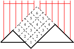
Figure 5. The path $\beta(3)$ of the length $N=12$ is drawn in bold. The corresponding factorised operator $H^{\rm A}_{3}$ is an ordered product of the Baxterised elements $h_{i}(u_{ij})$ represented by dashed tiles on the picture. The additional conditions (4.3) require that this picture vanishes.

Proposition 3.

The base coefficient function $\psi_{\Omega}^{\rm A}$ for the solution of the type A qKZ equation is subject to truncation relations

$$H^{\rm A}_{k}\,\psi_{\Omega}^{\rm A}=0\quad\forall\,k=1,2,\dots,\lfloor N/2\rfloor.$$ (4.3)

Conditions (3.16), (4.1), (4.2), (4.3) together are equivalent to the qKZ equations (3.1)-(3.3) of type A.

Proof.

Using the techniques described in the proof of Theorem 1, see

Section 6.1, it follows that the relations (4.3) ensure the vanishing of the contributions $\psi_{\alpha^{-}}$ in (3.19) if $\alpha^{-}$ is not a Dyck path, see Remark 5. Explicit examples are given in subsection 4.3. ∎

For a particular value of the boundary parameter $\lambda$ a simple polynomial solution of the conditions (4.3) was found in [12]:

Proposition 4.

For $\lambda=-3$, the conditions (4.3) admit the simple solution $\xi^{\rm A}=1$. In this case the coeficients of the qKZ equation, when properly normalised, are polynomials in variables $z_{i}=q^{x_{i}},\;\;i=1,\dots,N$.

Using the factorised formulas we have calculated these solutions for system sizes up to $N=10$. In the homogeneous limit $x_{i}\rightarrow 0$ the coefficients $\psi_{\alpha}(x_{1},\ldots,x_{N})$ become polynomials in $\tau=-[2]$. In fact, up to an overall factor, each $\psi_{\alpha}$ becomes a polynomial in $\tau^{2}$ with positive integer coefficients. These polynomials were considered in [14], where their intriguing combinatorial content was described. In Appendix B we present a table of these polynomials up to $N=10$, and we shall further discuss them in Section 5.

4.2. Type B

We will now formulate a factorised solution for type B. This result was deduced from some exercises we made for small size systems. As we found these instructive, we have given these in Appendix A. Analysing the expressions for the coefficient functions in the cases $N=2,3$ we see that in order to write them as a product of the Baxterised elements $h_{i}(u)$, $i\geq 0$, we have to fix in a special way the auxiliary parameter $\nu$ in the definition (3.12) of $h_{0}(u)$. From now on we therefore specify

$$\raisebox{-18.0pt}{\includegraphics[height=36.0pt]{h0.eps}}\,=\,\bar{h}_{0}(k)\,:=\,h_{0}(k)|_{\nu=\omega+p_{k}}\,=\,s_{0}-\frac{\left[\lfloor{k/2}\rfloor\right]\left[\omega+\lfloor{(k+1)/2}\rfloor\right]}{[k][\omega+1]},$$ (4.4)

where $p_{k}=k\mbox{~{}mod 2}$. Note that the Baxterised boundary element ${\bar{h}}_{0}(u)$ is defined for integer values of its spectral parameter $u\in{\mathbb{Z}}$ as only such values appear in our considerations.

Now we can repeat the procedure described in the beginning of Section 4.1 but with the set of Ballot paths instead of Dyck paths. For each Ballot path $\alpha$ we consider its complement to the maximal Ballot path $\Omega^{\rm B}$. This complement may be thought of as half a transpose symmetric Young diagram, cut along its symmetry axis. We fill the complement with (half-)tiles corresponding to the (boundary) Baxterised elements $h_{i}(u_{i,j})$ and ${\bar{h}}_{0}(u_{i,j})$ as shown in Figure 6.

Figure 6. Solution of the qKZ equation of type B. We use the graphical notation (2.19), (4.4) and (3.21) to represent the Baxterised elements $h_{i}(k)$, the boundary Baxterised elements ${\bar{h}}_{0}(k)$ and the coefficient $\psi_{\Omega}^{\rm B}$.

The rule for assigning integers $u_{i,j}$ to the tiles remains exactly the same as for type A. For the half-tiles the rule is:

• put $u_{0,j}=1$ if there is no adjacent tile $h_{1}$ with the coordinate $(1,j-1)$;

• otherwise, put $u_{0,j}=u_{1,j-1}+1$.

The operator $H_{\alpha}$ corresponding to the Ballot path $\alpha$ is given by the same formula (4.1) as for type A, where now index $i$ may take also value $0$, thus allowing the boundary operators ${\bar{h}}_{0}(u_{0,j})$ enter the product.

Theorem 2.

Let $\alpha$ be a Ballot path of length $N$. The corresponding coefficient $\psi_{\alpha}$ of the solution of type B qKZ equation is given by

$$\psi_{\alpha}=H_{\alpha}\psi_{\Omega}^{\rm B},$$ (4.5)

where $\psi_{\Omega}^{\rm B}$ is the base function corresponding to the maximal Ballot path $\Omega^{\rm B}$ of length $N$ and the factorised operator $H_{\alpha}$ is defined in (4.1), see also Figure 6.

The proof of Theorem 2 is given in Section 6.2.

4.2.1. Truncation conditions

For $k=1,\dots,n=\lfloor\tfrac{N+1}{2}\rfloor$, let $\gamma{(k)}$ denote the path of the length $N$ with only one minimum, occuring at the point $\,2k-\epsilon_{N}-1\,$ with ${\gamma(k)}_{2k-\epsilon_{N}-1}=-1\,$ (recall that $\epsilon_{N}=N\bmod 2$). Note that $\gamma(k)$ is therefore not a Ballot path. The associated half-Young diagram has a shape of trapezium. We introduce the notation $H^{\rm B}_{k}:=H_{\gamma{(k)}}$ for the corresponding factorised operator. An example of a path $\gamma{(k)}$ with $N=10$ and $k=3$ is shown in Figure 7.

Figure 7. The path $\gamma(3)$ of the length $N=10$ is drawn in bold. The corresponding factorised operator $H^{\rm B}_{3}$ is an ordered product of the Baxterised elements $h_{i}(u_{ij})$ represented by dashed tiles on the picture. The additional conditions (4.6) require that this picture vanishes.

Proposition 5.

The base coefficient function $\psi_{\Omega}^{\rm B}$ for the solution of the type B qKZ equation satisfies the truncation conditions

$$H^{\rm B}_{k}\,\psi_{\Omega}^{\rm B}\,=\,0\quad\forall\,k=1,2,\dots,n.$$ (4.6)

Conditions (3.20), (4.5) and (4.6) together are equivalent to the qKZ equations (3.1)-(3.3) of type B.

Proof.

Just as for type A, the relations (4.6) ensure the absence of $\psi_{\alpha^{-}}$ in (3.22) if $\alpha^{-}$ is not a Ballot path. Explicit examples are considered in Appendix A. ∎

For particular values of the boundary parameter $\lambda$ and the algebra parameter $\omega$ the simplest polynomial solution of the conditions (4.6) was found in [51]:

Proposition 6.

In case $\lambda=-3/2$ and $\omega=-1/2$ the conditions (4.6) admit the simple solution $\xi^{\rm B}=1$. In this case the coeficients of the qKZ equation, when properly normalised, become polynomials in variables $z_{i}=q^{x_{i}},\;\;i=1,\dots,N$.

4.3. Separation of truncation conditions

4.3.1. Type A

The equations (4.3) impose restrictions on the otherwise arbitrary symmetric functions $\xi^{\rm A}$ of the ansatz (3.16). Based on experience with calculations for small $N$ we observe that these restrictions can be written in a more explicit way. Namely, one can separate the functional part (depending on variables $x_{i}$) and the permutation part (depending on the permutations $\pi_{i}$) in the operators $H^{\rm A}_{k}$ in (4.3).

To formulate this separation in a precise way, let us first define the following set of Baxterised elements in the group algebra of the symmetric group ${\mathbb{C}}[S_{N}]\simeq\mathcal{H}^{\rm A}_{N}(1)$:

$$\pi_{i}(u):=u^{-1}-\pi_{i}\quad i=1,\dots,N-1.$$

Denote furthermore by $\Pi^{\rm A}_{k}$ the permutation operators obtained from the operators $H^{\rm A}_{k}$ by substituting $h_{i}(u_{i,j})\mapsto\pi_{i}(u_{i,j})$.

Conjecture 1.

The left hand side of the truncation condition (4.3) for Type A can be written in the following separated form (remind that $n=\lfloor\tfrac{N+1}{2}\rfloor$)

$$H^{\rm A}_{k}\psi_{\Omega}^{\rm A}=\frac{\Delta^{-}_{1}(x_{k},\dots,x_{n+k})}{\Delta^{-}_{0}(x_{k},\dots,x_{n+k})}\,\Pi^{\rm A}_{k}\,\frac{\Delta^{-}_{0}(x_{k},\dots,x_{n})\Delta^{-}_{0}(x_{n+1},\dots,x_{n+k})}{\Delta^{-}_{1}(x_{k},\dots,x_{n})\Delta^{-}_{1}(x_{n+1},\dots,x_{n+k})}\,\psi_{\Omega}^{\rm A}.$$ (4.7)

Example 1.

In the case $N=5$ there are two truncation conditions on the base function $\psi_{\Omega}^{\rm A}$:

• Condition (4.7) for $k=1$ reads

  $$h_{1}(1)h_{2}(2)h_{3}(3)\psi_{\Omega}^{\rm A}=\frac{\Delta^{-}_{1}(x_{1},\dots,x_{4})}{\Delta^{-}_{0}(x_{1},\dots,x_{4})}\,\Pi^{\rm A}_{1}\frac{\Delta^{-}_{0}(x_{1},x_{2},x_{3})}{\Delta^{-}_{1}(x_{1},x_{2},x_{3})}\psi_{\Omega}^{\rm A}=0,$$

  or, in terms of $\xi^{\rm A}$

  $$\Pi_{1}^{\rm A}\Bigl{\{}\Delta^{-}_{0}(x_{1},x_{2},x_{3})\Delta^{+}_{-1}(x_{1},x_{2},x_{3})\Delta^{-}_{1}(x_{4},x_{5})\hskip 133.72795pt$$

  $$\hskip 142.26378pt\Delta^{+}_{\lambda+1}(x_{4},x_{5})\xi^{\rm A}(x_{1},x_{2},x_{3}|x_{4}+\tfrac{\lambda}{2},x_{5}+\tfrac{\lambda}{2})\Bigr{\}}\,=\,0,$$ (4.8)

  where $\Pi^{\rm A}_{1}:=(1-\pi_{1})(\tfrac{1}{2}-\pi_{2})(\tfrac{1}{3}-\pi_{3})$. Since the function in braces in (4.8) is antisymmetric in the variables $x_{1},x_{2},x_{3},$ the operator $\Pi_{1}^{\rm A}$ in this formula can be equivalently substituted by

  $$\Pi^{\rm A}_{1}\;\mapsto\;(1-\pi_{3}+\pi_{2}\pi_{3}-\pi_{1}\pi_{2}\pi_{3}).$$ (4.9)

• Condition (4.7) for $k=2$ reads

  $$\hskip 17.07164pth_{3}(1)h_{2}(2)h_{4}(2)h_{3}(3)\psi_{\Omega}^{\rm A}=\frac{\Delta^{-}_{1}(x_{2},\dots,x_{5})}{\Delta^{-}_{0}(x_{2},\dots,x_{5})}\,\Pi^{\rm A}_{2}\frac{\Delta^{-}_{0}(x_{2},x_{3})\Delta^{-}_{0}(x_{4},x_{5})}{\Delta^{-}_{1}(x_{2},x_{3})\Delta^{-}_{1}(x_{4},x_{5})}\psi_{\Omega}^{\rm A}=0.$$

  or, in terms of $\xi^{\rm A}$

  $$\Pi_{2}^{\rm A}\Bigl{\{}\Delta^{-}_{0}(x_{1}+1,x_{2},x_{3})\Delta^{+}_{-1}(x_{1},x_{2},x_{3})\Delta^{-}_{0}(x_{4},x_{5})\hskip 133.72795pt$$

  $$\hskip 176.40707pt\Delta^{+}_{\lambda+1}(x_{4},x_{5})\xi^{\rm A}(x_{1},x_{2},x_{3}|x_{4}+\tfrac{\lambda}{2},x_{5}+\tfrac{\lambda}{2})\Bigr{\}}\,=\,0.$$

  The operator $\Pi^{\rm A}_{2}:=(1-\pi_{3})(\tfrac{1}{2}-\pi_{2})(\tfrac{1}{2}-\pi_{4})(\tfrac{1}{3}-\pi_{3})$ in this formula can be equivalently substituted by

  $$\Pi^{\rm A}_{2}\;\mapsto\;(1-\pi_{3}+\pi_{2}\pi_{3}+\pi_{4}\pi_{3}-\pi_{2}\pi_{4}\pi_{3}+\pi_{3}\pi_{2}\pi_{4}\pi_{3}).$$ (4.10)

Formulas (4.9), (4.10) suggest the following proposition

Proposition 7.

In condition (4.7) one can substitute the operator $\Pi^{\rm A}_{k}$ by a polynomial in the permutations $(-\pi_{i})$, $i=k,\dots,n+k-1$, with unit coefficients. The terms of the polynomial are labeled by the sub-diagrams of the rectangular Young diagram $\{k^{(n-k+1)}\}$ corresponding to the path $\beta(k)$, see subsection 4.1.1. Their form is given by formula (4.1), where one has to substitute the factors $h_{i}(u_{ij})$ by $-\pi_{i}$.

4.3.2. Type B

In this case we found analogues of the expressions (4.7) for particular truncation conditions (4.6) only.

Let us supplement the set of Baxterised elements $\pi_{i}(u)$ with the boundary Baxterised element

$$\pi_{0}(u):=u^{-1}-\pi_{0}.$$

The elements $\pi_{i}(u)$, $i=0,1$ satisfy a reflection equation of the form (2.17).

Denote by $\Pi^{\rm B}_{n}$ the operator obtained from $H^{\rm B}_{n}$ by the substitutions

$${\bar{h}}_{0}(u_{i,j})\mapsto\pi_{0}(1),\quad h_{i}(u_{i,j})\mapsto\pi_{i}(u_{i,j})\;\;\forall\,i\geq 1.$$

Conjecture 2.

The left hand side of the condition (4.6) for $k=n$ and arbitrary $N$ can be transformed to

$$H^{\rm B}_{n}\,\psi_{\Omega}^{\rm B}\,=\,\Bigl{\{}\frac{\Theta(x_{1},\dots,x_{N})\Delta^{-}_{1}(x_{1},\dots,x_{N})}{\Delta^{-}_{0}(x_{1},\dots,x_{N})}\,\Pi^{\rm B}_{n}\,\frac{\Delta^{-}_{0}(x_{2},\dots,x_{N})}{\Theta(x_{2},\dots,x_{N})\Delta^{-}_{1}(x_{2},\dots,x_{N})}\,-\,$$

$$\frac{[\lfloor N/2\rfloor][\omega+n]}{[\omega+1]}\Bigr{\}}\psi_{\Omega}^{\rm B}\,,\hskip 142.26378pt$$

where $n=\lfloor\tfrac{N+1}{2}\rfloor$ and $\Theta(x_{i},\ldots,x_{j}):=\prod_{i\leq p\leq j}\frac{k(x_{p},\,\delta)}{[2x_{p}][\omega+1]}\,$.

For $N$ odd denote by $\Pi^{\rm B}_{1}$ the operator obtained from $H^{\rm B}_{1}$ by the substitutions

$${\bar{h}}_{0}(u_{i,j})\mapsto\pi_{0}(u_{i,j}),\quad h_{i}(u_{i,j})\mapsto\pi_{i}(u_{i,j})\;\;\forall\,i\geq 1.$$

Conjecture 3.

The left hand side of the condition (4.6) for $k=1$ and $N$ odd can be written in the following separated form

$$H^{\rm B}_{1}\psi_{\Omega}^{\rm B}=\Theta(x_{1},\dots,x_{n})\frac{\Delta^{-}_{1}(x_{1},\dots,x_{n})\Delta^{+}_{-1}(x_{1},\dots,x_{n})}{\Delta^{-}_{0}(x_{1},\dots,x_{n})\Delta^{+}_{0}(x_{1},\dots,x_{n})}\,\Pi^{\rm B}_{1}\,\frac{\Delta^{-}_{0}(x_{1},\dots,x_{n})}{\Delta^{-}_{1}(x_{1},\dots,x_{n})}\,\psi_{\Omega}^{\rm B}.$$ (4.11)

Remark 6.

Notice that condition (4.11) does not actually depend on the algebra parameter $\omega$. If we choose $\xi^{\rm B}=1$, then it is satisfied for $\lambda\in\{-3/2,-2\}$ only.

5. Observations and conjectures

In this section we consider explicit polynomial solutions of the qKZ equation described in Propositions 4 and 6, and we consider the homogeneous limit $x_{i}\rightarrow 0$. We would like to emphasize the importance of these explicit solutions for experimentation and for the discovery of many interesting new results. In this section we formulate some of these observations. We present new positivity conjectures and relate partial sums over components to single components for larger system sizes. Furthermore, based on our results we have been able to find a compact expression for generalised partial sums in the inhomogeneous case.

5.1. Type A

In Appendix B we have listed the solutions described in Proposition 4 up to $N=10$ in the limit $x_{i}\rightarrow 0$, $i=1,\ldots,N$. These solutions were obtained using the factorised forms of the previous section.

In the following we will write shorthand $\psi_{\alpha}$ for the limit $x_{i}\rightarrow 0$ of $\psi_{\alpha}(x_{1},\ldots,x_{N})$. The complete solution is determined up to an overall normalisation. We will choose $\xi^{\rm A}=(-1)^{n(n-1)/2}$ where $n=\lfloor(N+1)/2\rfloor$ for which we have

$$\psi_{\Omega}^{\rm A}=\tau^{\lfloor{N/2}\rfloor(\lfloor N/2\rfloor-1)/2}.$$

An immediate observation was already noted in [14]:

Observation 1.

The components $\psi_{\alpha}(x_{1},\ldots,x_{N})$ of the polynomial solution of the qKZ equation of type A in the limit $x_{i}\rightarrow 0$, $i=1,\ldots,N$ are, up to an overall factor which is a power of $\tau$, polynomials in $\tau^{2}$ with positive integer coefficients. Here $\tau=-[2]$.

We now conjecture a partial combinatorial interpretation, by considering certain natural sums over subsets of Dyck paths. Let us first define the paths $\Omega(N,p)\in\mathcal{D}_{N}$ whose local minima lie on the height $\tilde{p}$, where

$$\tilde{p}=\lfloor{(N-1)/2}\rfloor-p.$$

Figure 8 illustrates the path $\Omega(12,3)$.

Figure 8. The minimal path $\Omega(12,3)\in\mathcal{D}_{12,3}$ .

For later convenience we also define, in the case of odd $N$, the paths $\widetilde{\Omega}(N,p)\in\mathcal{D}_{N}$ whose first $p-1$ local minima lie on the height $\tilde{p}$, except for the last minimum which lies at height 0. Figure 9 illustrates the path $\widetilde{\Omega}(13,4)$.

Figure 9. The path $\widetilde{\Omega}(13,4)\in\mathcal{D}_{13,6}$ .

We define the subset $\mathcal{D}_{N,p}$ of Dyck paths of length $N$ which lie above $\Omega(N,p)$, i.e. whose local minima lie on or above height $\tilde{p}$. Formally, this subset is described as

$$\mathcal{D}_{N,p}=\left\{\alpha\in\mathcal{D}_{N}|\ \alpha_{i}\geq\Omega_{i}(N,p)=\min(\Omega_{i},\tilde{p})\right\},$$

where $\Omega_{i}=\min\{i,N+\epsilon_{N}-i\}$, $\epsilon_{N}=N\bmod 2$, are integer heights of the maximal Dyck path $\Omega^{\rm A}=\Omega(N,0)$. We further define an integer $c_{\alpha,p}$ associated to each Dyck path in the following way (see also Appendix B). Let $\alpha=(\alpha_{0},\alpha_{1},\ldots,\alpha_{N})\in\mathcal{D}_{N,p}$ be a Dyck path of length $N$ whose minima lie on or above height $\tilde{p}$. Then $c_{\alpha,p}$ is defined as the signed sum of boxes between $\alpha$ and $\Omega(N,p)$, where the boxes at height $\tilde{p}+h$ are assigned $(-1)^{h-1}$ for $h\geq 1$. An example is given in Figure 10, and an explicit expression for $c_{\alpha,p}$ is given by

$$c_{\alpha,p}=\frac{(-1)^{\tilde{p}}}{2}\left(\sum_{i=1}^{\lfloor N/2\rfloor}(\alpha_{2i}-\Omega_{2i}(N,p))-\sum_{i=0}^{\lfloor(N-1)/2\rfloor}(\alpha_{2i+1}-\Omega_{2i+1}(N,p))\right).$$

Figure 10. Definition of the number $c_{\alpha,p}$ as the signed sum of boxes between the $\alpha$ and the path $\widetilde{\Omega}(12,4)$. In this figure $N=12$ and $p=4$ and $c_{\alpha,4}=4-3+1=2$.

Consider the partial weighted sums

$$S_{\pm}(N,p)=\sum_{\alpha\in\mathcal{D}_{N,p}}\tau^{\pm c_{\alpha,p}}\,\psi_{\alpha},.$$ (5.1)

It was noted in [36, 33] that for $\tau=1$ ($q={\rm e}^{2\pi{\rm i}/3}$), these partial sums for system size $N$, correspond to certain individual elements for size $N+1$. Here we observe that this correspondence holds also for arbitrary $\tau$: the partial sums $S_{\pm}(N,p)$ are up to an overall normalisation proportional to certain individual components $\psi_{\alpha}$ of the solution for system size $N+1$:

$$\begin{array}[]{|l|l|}\hline\cr S_{+}(4,1)=\psi_{\includegraphics[width=24.0pt]{5_012121.eps}}&S_{-}(4,1)=\tau^{-2}\psi_{\includegraphics[width=24.0pt]{5_010101.eps}}\\ \hline\cr&S_{-}(5,2)=\tau^{-2}\psi_{\,\includegraphics[width=28.0pt,viewport=0.0pt 0.0pt 180.67499pt 40.15pt,clip={true}]{6_0101010.eps}}\\ &S_{-}(5,1)=\tau^{-2}\psi_{\includegraphics[width=28.0pt,viewport=0.0pt -10.03749pt 180.67499pt 60.22499pt,clip={true}]{6_0121210.eps}}\\ \hline\cr S_{+}(6,2)=\psi_{\includegraphics[width=32.0pt,viewport=0.0pt -10.03749pt 210.78749pt 60.22499pt,clip={true}]{7_01212121.eps}}&S_{-}(6,2)=\tau^{-3}\psi_{\includegraphics[width=32.0pt,viewport=0.0pt -10.03749pt 210.78749pt 40.15pt,clip={true}]{7_01010101.eps}}\\ S_{+}(6,1)=\psi_{\includegraphics[width=32.0pt,viewport=0.0pt -10.03749pt 210.78749pt 90.3375pt,clip={true}]{7_01232321.eps}}&S_{-}(6,1)=\tau^{-3}\psi_{\includegraphics[width=32.0pt,viewport=0.0pt -10.03749pt 210.78749pt 60.22499pt,clip={true}]{7_01212101.eps}}\\ \hline\cr&S_{-}(7,3)=\tau^{-3}\psi_{\includegraphics[width=36.0pt,viewport=0.0pt -10.03749pt 240.9pt 40.15pt,clip={true}]{8_010101010.eps}}\\ &S_{-}(7,2)=\tau^{-3}\psi_{\includegraphics[width=36.0pt,viewport=0.0pt -10.03749pt 240.9pt 60.22499pt,clip={true}]{8_012121210.eps}}\\ &S_{-}(7,1)=\tau^{-3}\psi_{\includegraphics[width=36.0pt,viewport=0.0pt -10.03749pt 240.9pt 100.37498pt,clip={true}]{8_012323210.eps}}\\ \hline\cr S_{+}(8,3)=\psi_{\includegraphics[width=40.0pt,viewport=0.0pt -10.03749pt 271.0125pt 60.22499pt,clip={true}]{9_0121212121.eps}}&S_{-}(8,3)=\tau^{-4}\psi_{\includegraphics[width=40.0pt,viewport=0.0pt -10.03749pt 271.0125pt 40.15pt,clip={true}]{9_0101010101.eps}}\\ S_{+}(8,2)=\psi_{\includegraphics[width=40.0pt,viewport=0.0pt -10.03749pt 271.0125pt 90.3375pt,clip={true}]{9_0123232321.eps}}&S_{-}(8,2)=\tau^{-4}\psi_{\includegraphics[width=40.0pt,viewport=0.0pt -10.03749pt 271.0125pt 60.22499pt,clip={true}]{9_0121212101.eps}}\\ S_{+}(8,1)=\psi_{\includegraphics[width=40.0pt,viewport=0.0pt -10.03749pt 271.0125pt 120.45pt,clip={true}]{9_0123434321.eps}}&S_{-}(8,1)=\tau^{-4}\psi_{\includegraphics[width=40.0pt,viewport=0.0pt -10.03749pt 271.0125pt 100.37498pt,clip={true}]{9_0123232101.eps}}\\ \hline\cr\end{array}$$

We formalise this observation in the following conjecture:

Observation 2.

$$S_{+}(N,p) =\psi_{\Omega(N+1,p)},\quad N\ {\rm even}$$

$$S_{-}(N,p) =\tau^{-N/2}\,\psi_{\widetilde{\Omega}(N+1,p+1)},\quad N\ {\rm even}$$

$$\ S_{-}(N,p) =\tau^{-(N-1)/2}\,\psi_{\Omega(N+1,p)},\quad N\ {\rm odd}.$$

The weigthed partial sums were defined in (5.1) in an ad-hoc way. This was the way they were discovered when searching for relations as in Observation 2. In fact, these partial sums arise in a natural way as we will show now:

Observation 3.

The partial sums $S_{\pm}(N,p)$ are obtained from factorised expressions. In particular, let

$$P_{N}^{-} =\prod_{j=1}^{p}\prod_{i=j-1}^{p-1}h_{\tilde{p}+2i+j}(1+j),$$

$$P_{N}^{+} =\prod_{j=1}^{p}\prod_{i=j-1}^{p-1}h_{\tilde{p}+2i+j}(-1),$$

where the product is ordered as in Figures 11 and  12. Then we have

$$S_{\pm}(N,p)=\lim_{x_{i}\rightarrow 0}P_{N}^{\pm}\,\psi_{\Omega}^{\rm A}.$$ (5.2)

Figure 11. The partial sum $S_{+}(10,3)$ in factorised form.

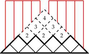
Figure 12. The partial sum $S_{-}(10,3)$ in factorised form.

In fact, we conjecture that (5.2) with (5.1) remain valid in the presence of the variables $x_{i}$:

Observation 4.

Define

$$P_{N}(u)=\prod_{j=1}^{p}\prod_{i=j-1}^{p-1}h_{\tilde{p}+2i+j}(u+j-1).$$

The weighted partial sums are special cases of the following identity for polynomials in $x_{1},\ldots,x_{N}$,

$$S(N,p,u):=P_{N}(u)\,\psi_{\Omega}^{\rm A}(x_{1},\ldots,x_{N})=\sum_{\alpha\in\mathcal{D}_{N,p}}\left(\frac{[1-u]}{[u]}\right)^{c_{\alpha,p}}\psi_{\alpha}(x_{1},\ldots,x_{N}).$$ (5.3)

Figure 13. The partial sum $S(10,3,u)$ in factorised form.

Note that (5.3) has many interesting specialisations, such as $u=0$ and $u=1$ which, when properly normalised, correspond to the single coefficients $\psi_{\Omega(N,\lfloor(N-1)/2\rfloor)}$ and    $\psi_{\Omega(N,\lfloor(N-3)/2\rfloor)}$ respectively. The standard sum rule where one performs an unweighted sum, corresponds to $u=1/2$. Interestingly, a special case of the generalised sum rule (5.3) is closely related to a result of [18], were a similar generalised sum was considered, based on totally different grounds and in the homogeneous limit $x_{i}\rightarrow 0$ and for $p=\lfloor(N-1)/2\rfloor$. By computation of a repeated contour integral, it was shown in [18] that in this case, $S(N,\lfloor(N-1)/2\rfloor,u)$ is equal to the generating function of refined $t,\tau$-enumeration of (modified) cyclically symmetric transpose complement plane parititions, where $t=[1-u]/[u]$. Because of the natural way this parameter appears in (5.3), we hope that this result offers further insights into the precise connection between solutions of the qKZ equation and plane partitions.

5.2. Type B

In Appendix B we have listed solutions of the qKZ equation for type B from Proposition 6 up to $N=6$ in the limit $x_{i}\rightarrow 0$, $i=1,\ldots,N$. These solutions were obtained using the factorised forms of the previous section. As in the case of type A, we again find a positivity conjecture, this time in the two variables $\tau^{\prime}$ and $a$ which are defined by

$$\tau^{\prime 2}=2-\tau=2+[2]=[2]_{q^{1/2}}^{2},\qquad a=\frac{[1/2]}{[\frac{2\delta+1}{4}][\frac{2\delta-1}{4}]}.$$

The complete solution is determined up to an overall normalisation. We will choose $\xi^{\rm B}=a^{\lfloor N/2\rfloor}(-\tau^{\prime 2})^{N(N-1)/2}$, for which we have

Observation 5.

The solutions $\psi_{\alpha}(x_{1},\ldots,x_{N})$ of the qKZ equation of type B in the limit $x_{i}\rightarrow 0$, $i=1,\ldots,N$ are polynomials in $\tau^{\prime 2}$ and $a$ with positive integer coefficients.

For $a=1$ this conjecture was already observed in [51]. As was conjectured in [11] for $\tau^{\prime}=1$, the parameter $a$ corresponds to a refined enumeration of vertically and horizontally symmetric alternating sign matrices. A sum rule for this value of $\tau^{\prime}$ was proved in [51]. We suspect that the parameter $\tau^{\prime}$ is related to a simple statistic on plane partitions, as it is for type A. We thus have an interesting mix of statistics, one which is natural for ASMs, and one which is natural for plane partitions. In a forthcoming paper we hope to formulate some further results concerning the solutions for type B.

6. Proofs

6.1. Proof of Theorem 1

We have to show that the vector $|\Psi\rangle$ whose coefficients are given by the formulas (3.16), and (4.1), (4.2) satisfies the qKZ equations (3.1)-(3.3) of type A. Following the preliminary analysis of Section 3.3.1 we divide the proof of (3.1) into two parts, depending on whether or not the word corresponding to the path $\alpha$ begins with $e_{i}$.

1. $\alpha$ does not have a local maximum at $i$. We have to show that, see (3.13),

$$-(a_{i}\psi_{\alpha})(x_{1},\ldots,x_{N})=(h_{i}(-1)\psi_{\alpha})(x_{1},\ldots,x_{N})=0$$ (6.1)

for $\psi_{\alpha}$ given by (4.2).

If $\alpha$ does not have a local maximum at $i$, then either $h_{i}(-1)$ acts on a local minimum, or on a slope of $\alpha$.

• $h_{i}(-1)$ acts on a local minimum of $\alpha$.

  In this case $\psi_{\alpha}$ is divisible by $h_{i}(1)$ from the left and (6.1) follows directly from

• $h_{i}(-1)$ acts on a slope of $\alpha$.

  In this case we use the Yang-Baxter equation (2.18) to push $h_{i}(-1)$ through the operator $H_{\alpha}$ (4.1) in the expression for $\psi_{\alpha}$ (4.2). Then $h_{i}(-1)$ vanishes when acting on $\psi_{\Omega}^{\rm A}$, see (3.18). This mechanism is illustrated in Figure 14.

  Figure 14. Action of $h_{i}(-1)$ on a slope of a Dyck path $\alpha$. The first equality follows from the Yang-Baxter equation (2.18) and the second follows from (3.18). For the operators $H_{\alpha}$ of a more general form (like, e.g., the one shown in Figure 4) the first part of this transformation should be repeated until $h_{i}(-1)$ commutes through all the terms of $H_{\alpha}$.

2. $\alpha$ has a local maximum at $i$. The harder part of the proof of Theorem 1, to which we come now, lies in proving (3.19) when $h_{i}(1)$ acts on a component $\psi_{\alpha}$ where the path $\alpha$ has local maximum at $i$. If this maximum at $i$ does not have a nearest neighbour minimum at $i-1$ or $i+1$ then (3.19) becomes simply

$$h_{i}(1)\psi_{\alpha}=\psi_{\alpha^{-}},$$

and the action of $h_{i}(1)$ is the addition of a tile with content $1$ at $i$, which is just the prescription of the Theorem 1, see Figure 15.

Figure 15. Graphical representation of the equation $h_{i}(1)\psi_{\alpha}=\psi_{\alpha^{-}}$ corresponding to the addition of a tile with content $1$ at a maximum without neighbouring minima. In this case $u>1$ and $v>1$.

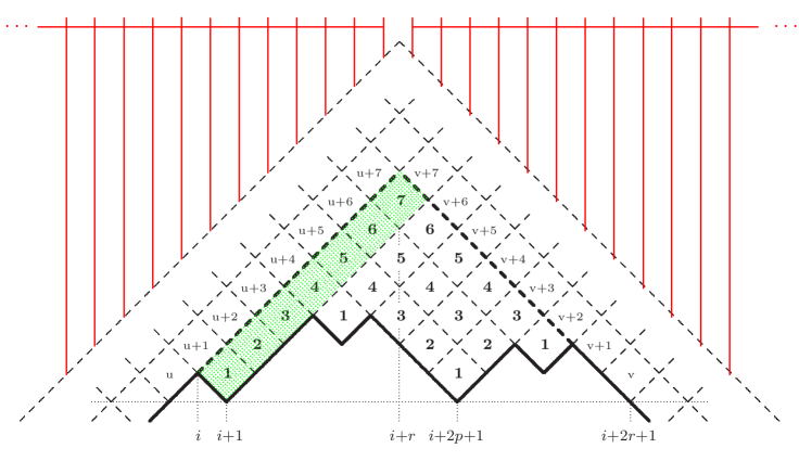
Figure 16. The Dyck path $\alpha$ satisfying conditions a) and b). Between $i+1$ and $i+2r+1$ this path contains exactly one local minimum at $i+2p+1$ which has the same height as the minimum at $i+1$.

We will now look at the action of $h_{i}(1)$ on $\psi_{\alpha}$ (4.2), where the Dyck path $\alpha$ satisfies conditions (see Figure 16)

• $\alpha$ has a maximum at $i$ with a neighbouring minimum at $i+1$;

• $\alpha$ crosses the horizontal line at height $\alpha_{i+1}=\alpha_{i}-1$, for the first time to the right of $i$, at $i+2r+1$, $r\geq 1$: $\alpha_{i+2r}-1=\alpha_{i+2r+1}=\alpha_{i+2r+2}+1=\alpha_{i+1}$.

In this case we observe that the factorised expression (4.2) for $\psi_{\alpha}$ contains a strip of tiles $H_{i+1,i+r}(1)$, where

$$H_{i+1,i+r}(u)\,:=\,h_{i+1}(u)h_{i+2}(u+1)\times\dots\times h_{i+r}(u+r-1).$$ (6.2)

This strip is shown shaded on Figure 16.

We are going to rewrite the term $h_{i}(1)H_{i+1,i+r}(1)$ in the product $h_{i}(1)\psi_{\alpha}$ in such a way that we obtain the components $\psi_{\alpha^{-}}$ and $\psi_{\alpha^{+k}}$ from the right hand side of (3.19), see also Figure 2, defined according to the rules (4.1), (4.2). As a first step we prove the following proposition:

Proposition 8.

Let $X$ be an arbitrary element of the algebra $\mathcal{H}^{\rm A}_{N}(q)$ taken in its faithful representation (3.2.1), (3.8). We denote by $A_{i,j}$, $i\leq j$, the linear span of terms $~{}Xa_{k}=Xh_{k}(-1)~{}$ $\forall\,k:i\leq k\leq j$. We define additionally $A_{i,i-1}:=0$,  $H_{i,i-1}(1):=1$.

The following relation is valid modulo $A_{i,i+r-1}\,$:

$$H_{i,i+r}(u)=H_{i,i+r}(u+v)\,+\,\frac{[v]}{[u][u+v]}\,H_{i+1,i+r}(1)\quad\mbox{\rm mod}\;A_{i,i+r-1}\qquad\forall\,r\geq 0\,.$$ (6.3)

For the proof of Proposition 8 we need the following two simple lemmas.

Lemma 2.

One has

1. $h_{i}(u)H_{i+1,i+r}(u+1)=H_{i,i+r}(u)$;

2. $H_{i,i+r}(u)h_{i+r+1}(u+r+1)=H_{i,i+r+1}(u)$;

3. for generic values of $\;u\,$ and $\,v$

   $$\hskip 25.60747ptH_{i,i+r}(u)=H_{i,i+r}(u+v)\\ +\sum_{k=0}^{r}\frac{[v]}{[u+k][u+v+k]}H_{i,i+k-1}(u+v)H_{i+k+1,i+r}(u+k+1)\,.$$ (6.4)

Proof.

The first two parts of the lemma follow immediately from the definition of $H_{i,i+r}(u)$ in (6.2). To prove (6.4) we use induction on $r$. For $r=0$ equation (6.4) reduces to (2.12). Now we shall make the inductive step by assuming (6.4) is true for some $r$, and prove it for $r+1$:

$$H_{i,i+r+1}(u)\, =\,H_{i,i+r}(u)h_{i+r+1}(u+r+1)\,=H_{i,i+r}(u+v)h_{i+r+1}(u+r+1)$$

$$\hphantom{=}+\sum_{k=0}^{r}\frac{[v]}{[u+k][u+v+k]}H_{i,i+k-1}(u+v)H_{i+k+1,i+r}(u+k+1)h_{i+r+1}(u+r+1)$$

$$=\,H_{i,i+r}(u+v)\left(h_{i+r+1}(u+v+r+1)+\frac{[v]}{[u+r+1][u+v+r+1]}\right)$$

$$\hphantom{=}+\sum_{k=0}^{r}\frac{[v]}{[u+k][u+v+k]}H_{i,i+k-1}(u+v)H_{i+k+1,i+r+1}(u+k+1)$$

$$=\,H_{i,i+r+1}(u+v)+\sum_{k=0}^{r+1}\frac{[v]}{[u+k][u+v+k]}H_{i,i+k-1}(u+v)H_{i+k+1,i+r+1}(u+k+1),$$

where we used (2.12) and the induction assumption. This completes the proof of Lemma 2. ∎

Lemma 3.

One has

$$H_{i,i+r}(u)\,=\,\frac{[u+r+1]}{[u]}\quad\mbox{\rm mod}\;A_{i,i+r}\,,$$ (6.5)

In particular, the coefficient $\psi_{\Omega}^{\rm A}$ (3.16) of the maximal Dyck path $\Omega^{\rm A}$ satisfies the relations

$$H_{i,i+r}(u)\,\psi_{\Omega}^{\rm A}\,=\,\frac{[u+r+1]}{[u]}\,\psi_{\Omega}^{\rm A},$$ (6.6)

in case the indices $\,r$ and $i$ are chosen within the limits $\,0\leq r<n-1\,$, $\,1\leq i<n-r$, where $n=\lfloor\tfrac{N+1}{2}\rfloor$.

Proof.

From (3.18) and (2.12) we find that

$$h_{i}(u)\,=\frac{[u+1]}{[u]}\,+h_{i}(-1)\,=\,\frac{[u+1]}{[u]}\quad\mbox{\rm mod}\;A_{i,i}\,,$$ (6.7)

which implies formula (6.5). Relation (6.6) for the coefficient $\psi_{\Omega}^{\rm A}$ then follows from (3.18). ∎

Proof of Proposition 8.

By applying (6.4) twice, first with the arguments $\{u,v\}$, and then with the arguments $\{u,v\}$ substituted by $\{u+1,-u\}$, we find:

$$H_{i,i+r}(u) =H_{i,i+r}(u+v)+\frac{[v]}{[u][u+v]}H_{i+1,i+r}(u+1)$$

$$\hskip 28.45274pt+\sum_{k=1}^{r}\frac{[v]}{[u+k][u+v+k]}H_{i,i+k-1}(u+v)H_{i+k+1,i+r}(u+k+1)$$

$$=H_{i,i+r}(u+v)+\frac{[v]}{[u][u+v]}H_{i+1,i+r}(1)$$

$$\hskip 28.45274pt-\frac{[v]}{[u][u+v]}\sum_{k=0}^{r-1}\frac{[u]}{[u+k+1][k+1]}H_{i+1,i+k}(1)H_{i+k+2,i+r}(u+k+2)$$

$$\hskip 28.45274pt+\sum_{k=1}^{r}\frac{[v]}{[u+k][u+v+k]}H_{i,i+k-1}(u+v)H_{i+k+1,i+r}(u+k+1)$$

$$=H_{i,i+r}(u+v)+\frac{[v]}{[u][u+v]}H_{i+1,i+r}(1)$$

$$+\sum_{k=1}^{r}\frac{[v]}{[u+k]}H_{i+k+1,i+r}(u+k+1)\left(\frac{1}{[u+v+k]}H_{i,i+k-1}(u+v)-\frac{1}{[u+v][k]}H_{i+1,i+k-1}(1)\right).$$ (6.8)

It lasts to notice that, by Lemma 3, the operators between parentheses in the last term of (6.8) become c-numbers modulo $A_{i,i+r-1}$ and in fact cancel:

$$\left(\frac{1}{[u+v+k]}H_{i,i+k-1}(u+v)-\frac{1}{[u+v][k]}H_{i+1,i+k-1}(1)\right)\\[2.84526pt] =\left(\frac{1}{[u+v+k]}\frac{[u+v+k]}{[u+v]}-\frac{1}{[u+v][k]}\frac{[k]}{[1]}\right)\quad\mbox{\rm mod}\;A_{i,i+r-1}\\ \,=\,0\quad\mbox{\rm mod}\;A_{i,i+r-1}\,.$$

Hence, (6.8) implies (6.3). ∎

Consider a path $\alpha$ whose all local minima between $i+1$ and $i+2r+1$ lie higher then $\alpha_{i+1}$. For such paths Proposition 8 implies the following

Corollary 3.

Let $\alpha=(\alpha_{0},\ldots,\alpha_{N})$ be a Dyck path satisfying conditions a) and b) on page 6.1. Assume additionally that $\alpha$ has no local minima at height $\alpha_{i+1}$ between $i+1$ and $i+2r+1$. Let further $\alpha^{-}$ (respectively, $\alpha^{+1}$) denote the path obtained from $\alpha$ by raising (resp., lowering) the height $\alpha_{i}$ (resp., $\alpha_{i+1}$) by two, see Figure 2. Then for the coefficients $\psi_{\alpha}$, $\psi_{\alpha^{-}}$, $\psi_{\alpha^{+1}}$ defined by (4.2) we have:

$$h_{i}(1)\psi_{\alpha}\,=\,\psi_{\alpha^{-}}+\psi_{\alpha^{+1}}\,.$$

Proof.

As we noted before, the product $h_{i}(1)\psi_{\alpha}$ contains the factor $h_{i}(1)H_{i+1,i+r}(1)$. Applying (6.3) and (6.7) for $u=v=1$, we can transform this factor in the following way

$$h_{i}(1)H_{i+1,i+r}(1) =\,h_{i}(1)H_{i+1,i+r}(2)\,+\,\frac{1}{[2]}h_{i}(1)H_{i+2,i+r}(1)\quad\mbox{\rm mod}\;A_{i+1,i+r-1}$$

$$=\,H_{i,i+r}(1)\,+\,H_{i+2,i+r}(1)\quad\mbox{\rm mod}\;A_{i,i+r-1}\,.$$ (6.9)

Upon substitution of this result back into $h_{i}(1)\psi_{\alpha}$ the terms containing the expressions $H_{i,i+r}(1)$ and $H_{i+2,i+r}(1)$ both assume the form of the ansatz (4.2). They correspond, respectively, to the paths $\alpha^{-}$ and $\alpha^{{}^{+}1}$. The terms from $A_{i,i+r-1}$ vanish due to the same mechanism as in Figure 14. This calculation is graphically displayed in Figure 17. ∎

Figure 17. Diagrammatic presentation of the Corollary 3. The transformation (6.9) is displayed in details.

Consider now a path $\alpha$ which has exactly one local minimum between $i+1$ and $i+2r+1$ of the same height as the minimum at $i+1$, see Figure 16. In this case the following Corollary holds.

Corollary 4.

Let $\alpha=(\alpha_{0},\ldots,\alpha_{N})$ be a Dyck path satisfying conditions a) and b) on page 6.1. Assume additionally that $\alpha$ has one local minimum placed at the point $(i+2p+1)$, $0<p<r$, which has exactly the same height as the minimum at $i+1$: $\alpha_{i+2p+1}=\alpha_{i+1}$, see Figure 16. Let further the paths $\alpha^{-}$, $\alpha^{+1}$ be defined as in Corollary 3, and denote by $\alpha^{+2}$ the path obtained from $\alpha$ by raising the heights $\alpha_{i+1},\dots,\alpha_{i+2p+1}$ by two, see Figure 2. Then for the coefficients $\psi_{\alpha}$, $\psi_{\alpha^{-}}$, $\psi_{\alpha^{+1}}$ and $\psi_{\alpha^{+2}}$ defined by (4.2) we have:

$$h_{i}(1)\psi_{\alpha}\,=\,\psi_{\alpha^{-}}+\psi_{\alpha^{+1}}+\psi_{\alpha^{+2}}\,.$$ (6.10)

Proof.

We copy the transformation of $h_{i}(1)\psi_{\alpha}$ from the proof of Corollary 3 till the end of (6.9). As before, the term $H_{i,i+r}(1)$ in the last line of (6.9) gives rise to the coefficient $\psi_{\alpha^{-}}\,$ in (6.10) whereas the term $A_{i,i+r-1}$ vanishes upon substitution into $h_{i}(1)\psi_{\alpha}$. This time however the term $H_{i+2,i+r}(1)$ when substituted into $h_{i}(1)\psi_{\alpha}$ does not give an expression fitting the ansatz (4.2). We continue its transformation using again (6.3) for $u=p$, $v=1$, and (6.5) for $u=1$:

$$H_{i+2,i+r}(1)\, =\,H_{i+2,i+p}(1)H_{i+p+1,i+r}(p)$$

$$=\,H_{i+2,i+p}(1)\Bigl{(}H_{i+p+1,i+r}(p+1)\,+\,\frac{1}{[p][p+1]}\,H_{i+p+2,i+r}(1)\Bigr{)}\quad\mbox{\rm mod}\;A_{i+p+1,i+r-1}$$

$$=H_{i+2,i+p}(1)H_{i+p+1,i+r}(p+1)\,+\,\frac{1}{[p+1]}\,H_{i+p+2,i+r}(1)\quad\mbox{\rm mod}\;A_{i+2,i+r-1}\,.$$ (6.11)

The first term in (6.11) upon substitution into $h_{i}(1)\psi_{\alpha}$ gives rise to the coefficient $\psi_{\alpha^{+1}}$, whereas the last term vanishes. It remains to consider the effect of the second term.

Let us introduce a further extension of the notation (6.2),

$$H_{i,i+r}^{\phantom{i,}i-s}(u) \,:=\,H_{i,i+r}(u)H_{i-1,i+r-1}(u+1)\times\dots\times H_{i-s,i+r-s}(u+s)\quad\forall\,r,s\geq 0,$$ (6.12)

$$H_{i,i-1}^{\phantom{i,}i-s} \,:=\,H_{i,i+r}^{\phantom{i,}i-1}\,:=\,1\,.$$

Graphically $H_{i,i+r}^{\phantom{i,}i-s}(u)$ can be displayed as a rectangular block of tiles of a size $(r+1)\times(s+1)$ with the bottom corner tile corresponding to $h_{i}(u)$. We also use the following shorthand symbols for uphill and downhill strips (the case of block with either $s=0$, or $r=0$):

$$H_{i,i+r}^{\phantom{i,}i}(u)\,:=\,H_{i,i+r}(u)\,,\qquad H_{i,i}^{\phantom{i,}i-s}(u)\,:=\,H_{i}^{i-s}(u)\,.$$

We now notice that in the assumptions of the Corollary the strip of tiles $H_{i+1,i+r}(1)$ in expression (4.2) for $\psi_{\alpha}$ is in fact multiplied from the left by the block of tiles $\raisebox{-5.69054pt}{\rule{0.0pt}{18.49428pt}}H_{i+2p+1,i+p+r}^{\phantom{i+2p+2,}i+p+2}(1)$. Therefore, we can continue the transformation of the second term in (6.11) by multiplying it from the left by the term $H_{i+2p+1,i+p+r}^{\phantom{i+2p+1,}i+p+2}(1)$. The transformation is essentially a permutation of these two terms which makes use of the Yang-Baxter equation (2.18):

$$H_{i+2p+1,i+p+r}^{\phantom{i+2p+1,}i+p+2}(1) \left(\frac{1}{[p+1]}\,H_{i+p+2,i+r}(1)\right)$$

$$=\, \frac{1}{[p+1]}\,H_{i+2p+2,i+p+r}(1)\,H_{i+2p+1,i+p+r-1}^{\phantom{i+2p+1,}i+p+2}(2)\,H_{i+p+r}^{i+r+1}(1)$$

$$=\, H_{i+2p+2,i+p+r}^{\phantom{i+2p+2,}i+p+2}(1)\quad\mbox{\rm mod}\;A_{i+r+1,i+p+r}\,.$$ (6.13)

Here in the last line we evaluate factor $H_{i+p+r}^{i+r+1}(1)$ using (6.5). The transformation (6.13) is illustrated in Figure 18.

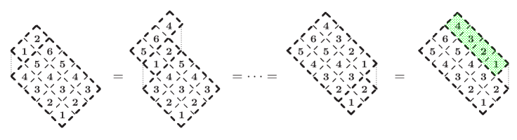
Figure 18. Diagrammatic presentation of the transformation (6.13) for the case $p=4$ and $r=7$ (this situation occurs in the third line of the calculation in Figure 19). Using the Yang-Baxter equation one moves the strip $H_{i+p+2,i+r}(1)$ down and right. The contents of the tiles in the block $H_{i+2p+2,i+p+r}^{\hskip 30.0pti+p+2}(1)$ are shifted cyclically in the uphill layers during the permutation. The shaded downhill strip $H_{i+p+r}^{i+r+1}(1)$ equals $[p+1]$ modulo $A_{i+r+1,i+p+r}$.

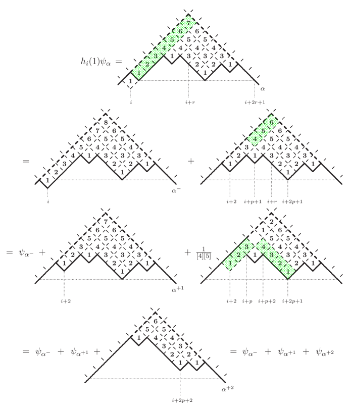
Figure 19. Diagrammatic illustration for the proof of Corollary 4. The path $\alpha$ is taken from Figure 16. Each time the transformation is applied to the strips which are shown shaded on the pictures. The second line on the Figure represents transformation (6.9). The third line corresponds to the transformation (6.11). The shaded uphill strip in this line can be evaluated as $\,[4]$ (cf. with the last equality in (6.11)). The shaded downhill strip has to be moved up and right (see Fig. 18) and then evaluated as $[5]$.

Substitution of the result of (6.13) back into $h_{i}(1)\psi_{\alpha}$ gives exactly the expression for the coefficient $\psi_{\alpha^{+2}}$. The whole calculation is graphically displayed in Figure 19. ∎

The general structure now is clear and we can formulate

Proposition 9.

Let $\alpha=(\alpha_{0},\ldots,\alpha_{N})$ be a Dyck path satisfying conditions a) and b) on page 6.1. Assume additionally that $\alpha$ has $K\geq 1$ local minima placed at the points $i+2p_{k}+1$, $0=p_{1}<\dots<p_{K}<r$, which have the same height $h=\alpha_{i+1}=\alpha_{i+2p_{k}+1}\;\forall k$, see Figure 2. Then for the coefficients $\psi_{\alpha}$, $\psi_{\alpha^{-}}$, $\psi_{\alpha^{+k}}$, $k=1,\dots,K,$ defined by (4.2) we have:

$$h_{i}(1)\psi_{\alpha}=\psi_{\alpha^{-}}+\sum_{k=1}^{K}\psi_{\alpha^{+k}},$$

where $\alpha^{-}$ and $\alpha^{+k}$ are the Dyck paths defined in Figure 2.

For the proof of Proposition 9 we need a generalisation of the formula (6.3) for the case of blocks (but now for $v=1$ only):

Lemma 4.

For generic values of $\;u\,$ one has

$$H_{i,i+r}^{\phantom{i,}i-s}(u)=H_{i,i+r}^{\phantom{i,}i-s}(u+1)\,+\,\frac{1}{[u][u+1]}\, H_{i+1,i+r}(1)\,H_{i-1}^{i-s}(1)\,H_{i,i+r-1}^{\phantom{i,}i-s+1}(u+2)$$

$$\hskip 19.91692pt\mbox{\rm mod}\;A_{i-s,i+r-s-1}\oplus A_{i+r-s+1,i+r}\,.$$ (6.14)

The graphical presentation of relation (6.14) given in Figure 20 is probably more clarifying.

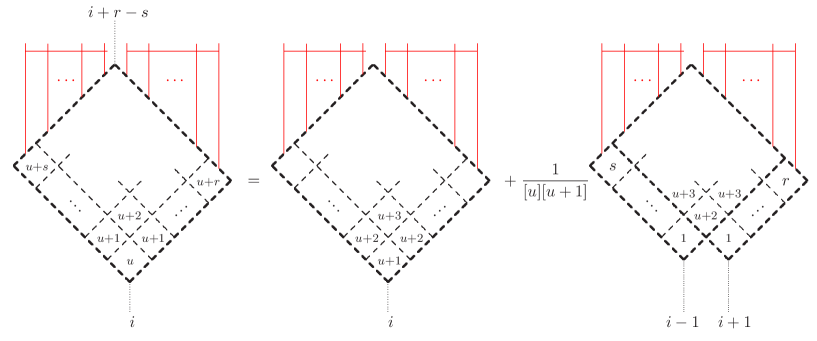
Figure 20. Diagrammatic presentation of relation (6.14). The colored vertical lines on top of the tilted rectangles symbolize annihilator of the terms $A_{i-s,i+r-s-1}$ and $A_{i+r-s+1,i+r}$. In the expressions for $\psi_{\alpha}$ (4.2) this role is played by the coefficient $\psi^{\rm A}_{\Omega}$.

Proof.

We use induction on $s$. For $s=0$ relation (6.14) reduces to (6.4). We now check it for some $s>0$ assuming it is valid for smaller values of $s$:

$$H_{i,i+r}^{\phantom{i,}i-s}(u)\,= \;H_{i,i+r}(u)H_{i-1,i+r-1}^{\phantom{i-1,}i-s}(u+1)$$

$$= \;\Bigl{(}H_{i,i+r}(u+1)\,+\,\frac{1}{[u][u+1]}\,H_{i+1,i+r}(1)\Bigr{)}H_{i-1,i+r-1}^{\phantom{i-1,}i-s}(u+1)\quad\mbox{\rm mod}\;A_{i-s,i+r-s-1}$$

$$= \;H_{i,i+r}(u+1)\,H_{i-1,i+r-1}^{\phantom{i-1,}i-s}(u+2)$$

$$+\,\frac{1}{[u+1][u+2]}\Bigl{(}H_{i,i+r}(u+1)\,H_{i,i+r-1}(1)\Bigr{)}H_{i-2}^{i-s}(1)\,H_{i-1,i+r-2}^{\phantom{i-1,}i-s+1}(u+3)$$

$$+\,\frac{1}{[u][u+1]}\,H_{i+1,i+r}(1)H_{i-1,i+r-1}^{\phantom{i-1,}i-s}(u+1)\;\;\mbox{\rm mod}\;A_{i-s,i+r-s-1}\oplus A_{i+r-s+1,i+r-1}$$

$$= \;H_{i,i+r-1}^{\phantom{i,}i-s+1}(u+1)$$

$$+\,\frac{1}{[u][u+1]}\,H_{i+1,i+r}(1)\Bigl{(}\frac{[u]}{[u+1]}H_{i-2}^{i-s}(1)\,+\,H_{i-1}^{i-s}(u+1)\Bigr{)}H_{i,i+r-1}^{\phantom{i,}i-s+1}(u+2)$$

$$\hskip 216.24094pt\mbox{\rm mod}\;A_{i-s,i+r-s-1}\oplus A_{i+r-s+1,i+r}$$

Here in the second line we used (6.3) for $v=1$ and take into account the fact

$$A_{i,I+r-1}\,H_{i-1,i+r-1}^{\phantom{i-1,}i-s}(u+1)\,\subset\,A_{i-s,i+r-s-1}\,.$$

When passing to the third line we used the induction assumption and then permuted two terms in parentheses in the fourth line using the Yang-Baxter equation (2.18). The result of this permutation contains the rightmost factor $h_{i+r}(u+1)$ which can be evaluated as $\,[u+1]/[u]$ modulo $A_{i+r}$. Finally, we notice that by obvious symmetry arguments the mirror images of relations (6.3) are valid for the downhill strips $H_{i}^{j}(u)$. Therefore, the term taken in parentheses in the last line equals $H_{i-1}^{i-s}(1)$. ∎

Proof of Proposition 9.

The simpler cases $K=1,2$ were already considered in Corollaries 3 and 4. In general the calculation of $h_{i}(1)\psi_{\alpha}$ can be carried out in the following steps:

Step 1.  Using the transformation (6.9) we extract the term $\psi_{\alpha^{-}}$ from $h_{i}(1)\psi_{\alpha}$. The residual term equals $\psi_{\alpha^{+1}}$ in case $K=1$, see Corollary 3.

Step 2.  In case $K>1$ the residue needs further transformation. Namely, to fit the ansatz (4.2) one has to rise by one the arguments in all tiles of the strip contained between the uphill lines starting at height $h=\alpha_{i+1}$ at points $i-1$ and $i+2p_{1}+1\equiv i+1$ and the downhill lines starting at the same height $h$ at points $i+2p_{2}+1$ and $i+2r+1$ (see the dashed strip in the picture in the second line of Figure 19). Acting in this way we extract the coefficient $\psi_{\alpha^{+1}}$ from the first step residue, see (6.11), and the rest, in case $K=2$, can be easily transformed to the form of $\psi_{\alpha^{+2}}$, see Figure 19.

Step 3.  In case $K>2$ the residual term of the second step does not fit the the ansatz (4.2) and has to be further transformed. This time one has to rise by one the arguments in the block of tiles contained between the uphill lines crossing the points $i-1$ and $i+2p_{2}+1$ at the height $h$ and the downhill lines crossing the points $i+2p_{3}+1$ and $i+2r+1$ at the same height. An example of the second step residue is given in Figure 21.

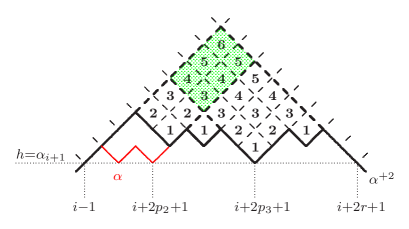
Figure 21. The case $K=3$, a typical diagram of the second step residue. The term which needs further transformation is the shaded block of tiles.

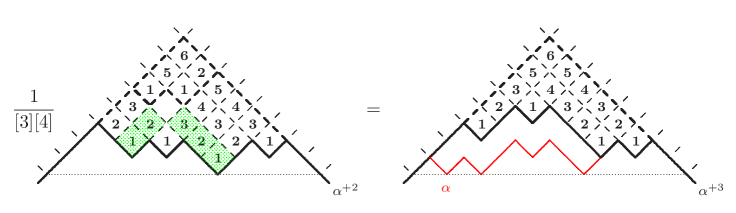
Figure 22. Transformation of the third step residue in case when the second step residue is given by Figure 21. Using the Yang-Baxter equation (2.18) shaded uphill/downhill strip can be moved up and left/right (see explanation in Figure 18) and then evaluated with the use of (6.5). Since $K=3$ in this example, the third step residue equals $\psi_{\alpha^{+3}}$.

We can raise the arguments in the block using the result of Lemma 4, see (6.14) and Figure 20. The first term from the right hand side of (6.14) gives rise to the coefficient $\psi_{\alpha^{+2}}$. The second term is the third step residue which can be further simplified using the Yang-Baxter equation (2.18) and the evaluation relation (6.5). In case $K=3$ the result of the transformation coincides with $\psi_{\alpha^{+3}}$. For the example of Figure 21 the transformation is illustrated in Figure 22.

From now on the consideration acquires its full generality and we continue the transformation until it ends up at Step $K$. ∎

Up to now we have finished the proof of the bulk qKZ equation (3.19) for the coefficients $\psi_{\alpha}$ whose corresponding Dyck paths $\alpha$ have a local maximum at $i$ and a neighbouring local minimum at $i+1$. Consideration of the cases where $\alpha$ has a neighbouring local minima at $i-1$, or both at $i-1$ and $i+1$ is a repetition of the same arguments.

It lasts to check the type A boundary qKZ relations (3.2) and (3.3). By Corollary 1 these conditions are verified by the coefficient $\psi_{\Omega}^{\rm A}$ of the maximal Dyck path. We then notice that none of the factors of the operator $H_{\alpha}$ (4.1) affect the coordinates $x_{1}$ and $x_{N}$ and hence commute with the boundary reflections $\pi_{0}$ and $\pi_{N}$, see (3.4) and(3.5). Therefore, each of the coefficients $\psi_{\alpha}=H_{\alpha}\psi_{\Omega}^{\rm A}$ (4.2) also satisfies the conditions (3.2) and (3.3).

This completes the proof of Theorem 1.

6.2. Proof of Theorem 2

The proof is analogous to that of Theorem 1 for type A, except that now we also have to make use of the reflection equation (2.20) for $\bar{h}_{0}$. Again, following the preliminary analysis of the Section 3.3.1 we divide the proof of (3.1) into two parts.

1.  In case $\alpha$ does not have a local maximum at $i$ we have to show that (6.1) is satisfied for $\psi_{\alpha}$ given by (4.5). The working is identical to that in type A, see Section 6.1, except for the case when $h_{i}(-1)$ acts on an uphill slope starting at the left boundary. In this case we additionally use (2.20) to reflect $h_{1}(-1)$ at the boundary, see the illustration on Figure 23.

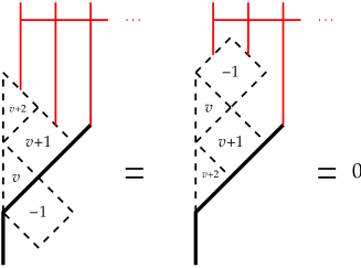
Figure 23. Reflection of $h_{1}(-1)$ at the origin. The first equality follows from the reflection equation (2.20) and the second one is a property of $\psi^{\rm B}_{\Omega}$ (3.20): $h_{1}(-1)\psi^{\rm B}_{\Omega}=0$.

2. If $\alpha$ has a local maximum at $i$, then we need to prove that Theorem 2 implies (3.22). Here again, the working is identical to that in type A except for the case where $\alpha$ has a local minimum at $i-1$ and has no lower local minima between $0$ and $i-1$. In this case, (3.22) contains the term $\psi_{\alpha^{+0}}$ which originates from reflections at the left boundary. The proof still follows basically the same lines as in type A although the calculations become quite elaborate. Therefore we decided to collect the necessary technical tools in the Lemma below and then to illustrate the idea of the proof on a few examples in pictures.

Let us introduce the following notation:

$$H_{0,i}(u)\, :=\,\bar{h}_{0}(u)\,H_{1,i}(u+1)\,,\qquad\quad H^{0}_{i}(u)\,:=\,H^{1}_{i}(u)\,\bar{h}_{0}(u+i)\,,$$

$$T_{0,i}(u)\, :=\,H_{0,i}(u)\times H_{0,i-1}(u+2)\times\dots\times H_{0,1}(u+2i-2)\times\bar{h}_{0}(u+2i)\,.$$

Pictorially $H_{0,i}(u)$ and $H^{0}_{i}(u)$ can be displayed as uphill and downhill strips starting with the half-tile at the left boundary, and $T_{0,i}(u)$ is a right triangle whose hypotenuse lies on the left boundary vertical line. We also extend the domain of definition for $\bar{h}_{0}(u)$ (4.4) demanding that

$$\bar{h}_{0}(0)\,:=\,s_{0}\,-\,\frac{[\omega]}{2[\omega+1]}\,.$$ (6.15)

For the newly introduced quantities the following analogues of equation (6.9) and Lemma 4 hold

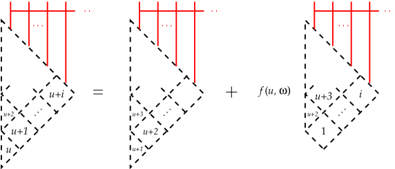
Figure 24. Diagrammatic presentation of (6.14). The coloured vertical lines on top of the tilted triangles annihilate the term $A_{1,i}$.

Lemma 5.

One has

1. $$\mbox{\rm 1.}\quad h_{i}(1)\,H_{i-1}^{0}(1)\,=\,H_{i}^{0}(1)\,+\,H_{i-2}^{0}(1)\,+\,c_{0}(i)\quad\mbox{\rm mod}\,A_{1,i}\,\quad\forall\,i=1,2,\dots,$$ (6.16)

   
   

   where $c_{0}(i)=1$ if $i$ is odd, $c_{0}(i)=-\tfrac{[\omega]}{[\omega+1]}$ if $i$ is even, and we assume $H_{-1}^{0}(1)=0$;

2. for nonnegative integers $\;i\,$ and $\;u\,$

   $$T_{0,i}(u)\,=\,T_{0,i}(u+1)\,+\,f(u,\omega)\,H_{1,i}(1)\,T_{0,i-1}(u+2)\,,$$ (6.17)

   where 

   $$f(u,\omega)=\left\{\begin{array}[]{rl}\displaystyle-\,\frac{[\omega]}{2[\omega+1]}&\mbox{if\; $u=0$,}\\[5.69054pt] \displaystyle\frac{[p][p-\omega]}{[2p][2p+1][\omega+1]}&\mbox{if\; $u=2p$\; is even positive,}\\[5.69054pt] \displaystyle\frac{[p][p+\omega]}{[2p-1][2p][\omega+1]}&\mbox{if\; $u=2p-1$\; is odd.}\end{array}\right.\vspace{1mm}$$ (6.18)

   and we assume $H_{1,0}(1)=T_{0,-1}(u)=1$.

Equation (6.17) is displayed graphically in Figure 24.

Proof.

Equations (6.16) follow easily from (the mirror images of) (6.3), (6.5), and from (4.4). Relations (6.17) can be proved by induction. The considerations are standard and we just briefly comment on them.

For $i=0$, (6.17) follows from (4.4). To check the induction step $i\rightarrow i+1$ one makes a decomposition

$$T_{0,i+1}(u)\,=\,\bar{h}_{0}(u)\,H_{1,i+1}(u+1)\,T_{0,i}(u+2)$$

and applies formulas (6.3), (4.4) and the induction assumption to rise consecutively the contents by one of the factors $H_{1,i+1}(u+1)$, $\bar{h}_{0}(u)$ and $T_{0,i}(u+2)$. Recollecting the (half-)tiles in the resulting expressions with the help of the Yang-Baxter equation (2.18) and the reflection equation (2.20), and using the evaluation formulas (6.5) and (4.4) together with its consequence

$$\bar{h}_{0}(u)\bar{h}_{0}(u+2)\,=\,a\,\bar{h}_{0}(u+2)\,+\,b\qquad\mbox{(for some numbers $a$ and $b$),}$$

one finally reproduces the term $T_{0,i+1}(u+1)$ and a combination of terms $H_{1,i+1}(u+1)T_{0,i}(u+2)$ and $H_{2,i+1}(1)T_{0,i}(u+2)$. The latter can be simplified to $H_{1,i+1}(1)T_{0,i}(u+2)$, thanks to the relations (6.4). The unwanted terms $H_{2,i+1}(1)H_{1,i}(u+3)T_{0,i-1}(u+4)$ appearing at the intermediate steps cancel in the final expression.

We mention here that all manipulations with q-numbers, which one needs during the transformation, can be easily done with the help of the following identities

$$[u+k][v\pm k]\,=\,[u][v]\,+\,[k][v\pm(u+k)]\,.$$ (6.19)

∎

We now continue the proof of (3.22).

Consider the action of $h_{i}(1)$ on the Ballot path $\alpha$ which has a local minimum at $i-1$ and all the local minima in between $0$ and $i-1$ are higher then $\alpha_{i-1}$. In this case, applying relation (6.16), we find

$$h_{i}(1)\psi_{\alpha}\,=\,\psi_{\alpha^{-}}\,+\,\psi_{\alpha^{+1}}\,+\,\psi_{\alpha^{+0}}\,,$$ (6.20)

where the paths $\alpha^{-}$, $\alpha^{+0/1}$ are defined in Figure 3 and their corresponding coefficients are given by (4.5). Note that, according to Lemma 5.1, in the case $i=1$ the term $\psi_{\alpha^{+1}}$ should be absent from the right hand side of (6.20). Altogether these prescriptions are identical to those of (3.22). The transformation (6.20) is illustrated in Figure 25.

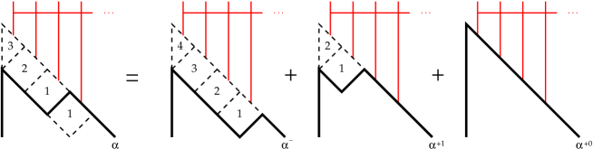
Figure 25. Diagrammatic presentation of relation (6.20). In the case shown on Figure $i=3$ and, hence, the coefficient in front of $\psi_{\alpha^{+0}}$ equals $1$.

We now consider the case where the path $\alpha$ contains $m\geq 1$ local minima between $0$ and $i-1$ which are of the same height as the minimum at $i-1$. The proof can be carried out in $K=m+2$ steps (cf. the proof of Proposition 9). To explain the first three steps we consider the case $m=1$, i.e., a path $\alpha$ with the two local minima placed at $i-1$ and $i-2p-1$, $p>0\,$: $\alpha_{i-2p-1}=\alpha_{i-1}$. Examples of such paths are given in Figure 26.

a) $$i p=\tfrac{i-1}{2} i p=\small\tfrac{i}{2}-1 i=8 p=2$$ odd and b) even and c) ,

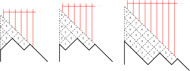
Figure 26. Ballot paths $\alpha$ with two local minima of the same height, one at $i-1$ and another one at $i-2p-1$. In these cases one calculates $h_{i}(1)\psi_{\alpha}$ in $K=3$ steps.

The calculation of $h_{i}(1)\psi_{\alpha}$ for the path shown on Figure 26 c) is illustrated in Figures 27–30.

Step 1.  Extraction of coefficient $\psi_{\alpha^{-}}$ from $h_{i}(1)\psi_{\alpha}$, see Figure 27.

We use (6.9) to raise by one the contents in the shaded strip $H_{i-1}^{1}(1)$ on Figure 27. The result is a sum of two terms. The second term is a residue of the first step which is to be further transformed at the second step. We denote it by $R_{1}$. Here we transform the first term raising by one the content of its top half-tile $\bar{h}_{0}(i)$ (shown shaded on Figure 27) with the help of (6.17). This results in a sum of $\psi_{\alpha^{-}}$ and a term proportional to $\psi_{\alpha^{+0}}$, see the second line in Figure 27. The factor $[9]$ in the coefficient of $\psi_{\alpha^{+0}}$ comes from the evaluation of the top strip $H_{i}^{1}(1)$.

$h_{i}(1)\psi_{\alpha}\,=\,$

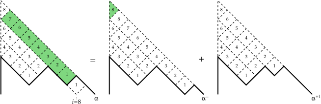
$$=\,\psi_{\alpha^{-}}\,+\,[9]\,\frac{[4][4-\omega]}{[8][9][\omega+1]}\,\psi_{\alpha^{+0}}\,+\,R_{1}$$

Figure 27. Extraction of the coefficient $\psi_{\alpha^{-}}$ from the expression $h_{i}(1)\psi_{\alpha}$.

$$\psi_{\alpha^{+1}}\,+\,\frac{1}{[3]} R_{1}\;=\;$$

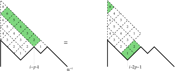
$$=\,\psi_{\alpha^{+1}}\,+\,\frac{[5]}{[3]}\,\Bigl{(}\frac{1}{[2]}-\frac{[4][\omega+4]}{[8][\omega+1]}\Bigr{)}\,\psi_{\alpha^{+0}}\,+\,R_{2}$$

Figure 28. Extraction of coefficient $\psi_{\alpha^{+1}}$ from $R_{1}$.

Step 2.  Extraction of coefficient $\psi_{\alpha^{+1}}$ from the first step residue, see Figure 28.

Again, we use (6.9) to raise by one the contents in the shaded strip $H_{i-p-1}^{1}(p)$ on Figure 28. The result is a sum of $\psi_{\alpha^{+1}}$ and a term which we continue transforming. Using the definition of $\bar{h}_{0}$ (4.4) we lower the content of the top half-tile (shown shaded) from $i$ to $i-2p-2$ (from $8$ to $2$ in the particular case shown on Figure 28) :

$$\bar{h}_{0}(8)\,=\,\left(\tfrac{1}{[2]}-\tfrac{[4][\omega+4]}{[8][\omega+1]}\right)\,+\,\bar{h}_{0}(2)\,.$$ (6.21)

The constant term resulting from this procedure gives a contribution proportional to $\psi^{\alpha^{+0}}$, see the second line of Figure 28. The factor $[5]$ appearing in the coefficient of $\psi_{\alpha^{+0}}$ is due to the evaluation of the top strip $H_{4}^{1}(1)$ (in general one evaluates $H_{i-p-2}^{1}(1)\rightarrow[i-p-1]$).

Lowering of the content in the top half-tile allows us to reorder the (half-)tiles of the last term in the first line of Figure 28. Namely, analogously to the case considered in Figure 18 we can push the uphill strip $H_{i-2p-1,i-p-2}(1)$ (shown shaded) up and left using the Yang-Baxter equation until it touches the left boundary. Then we reflect the strip at the boundary as shown on Figure 29, which is possible because we changed the content of $\bar{h}_{0}$ from 8 to 2 in (6.21). Finally, after reflection, the strip can be evaluated, cancelling the numeric factor in front of the picture. We call the result of this transformation a residue of the second step and denote it by $R_{2}$.

Figure 29. Reflection of a strip at the boundary. Here we use the Yang-Baxter equation (2.18) in the first and the last equalities and the reflection equation (2.20) in the second equality. The shaded downhill strip equals $[3]$ modulo $A_{1,2}$.

Step 3.  Extraction of coefficient $\psi_{\alpha^{+2}}$ from the second step residue, see Figure 30.

We use (6.17), see also Figure 24 to increase the contents of the triangle $T_{0,p}(i-2p-2)$ (shown shaded on the figure). The result is a sum of $\psi_{\alpha^{+2}}$ and a term which in fact is proportional to $\psi_{\alpha^{+0}}$. To prove this, one has to push up the downhill strip $H_{i-2p-2}^{1}(1)$ (shown shaded on the figure) and then evaluate it in the same way as it was done in the transformation (6.9), see Figure 18.

$$=\,\psi_{\alpha^{+2}}+\frac{[1-\omega]}{[2][3][\omega+1]} R_{2}\;=\;$$

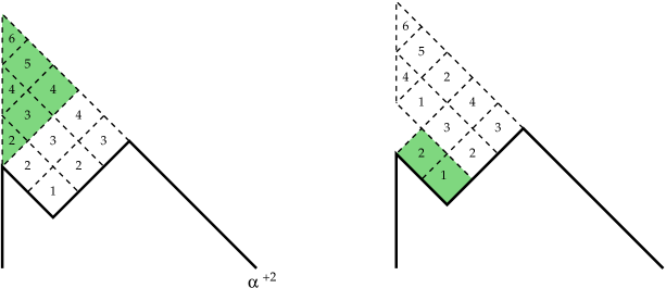
$$=\,\psi_{\alpha^{+2}}\,+\,\frac{[1-\omega]}{[2][\omega+1]}\,\psi_{\alpha^{+0}}$$

Figure 30. Extraction of coefficient $\psi_{\alpha^{+2}}$ from $R_{2}$.

Finally, collecting the terms $\psi_{\alpha^{+0}}$ from all three steps we find

$$h_{i}(1)\psi_{\alpha}\,=\,\psi_{\alpha^{-}}\,+\,c_{0}(i)\,\psi_{\alpha^{+0}}\,+\,\psi_{\alpha^{+1}}\,+\,\psi_{\alpha^{+2}}\,,$$ (6.22)

where $c_{0}(i)=-\tfrac{[\omega]}{[\omega+1]}$ for the particular case considered in Figures 27–30. This value holds for all cases with $i$ even, while $c_{0}(i)=1$ for all cases with $i$ odd. In general, the coefficient $c_{0}(i)$ can be calculated with the help of (6.19).

Equations (6.22) coincide with the prescriptions of (3.22) in case the path $\alpha$ contains $m=1$ local minimum between $0$ and $i-1$ of the same height as the minimum at $i-1$. Before we proceed to cases with $m\geq 2$ let us comment on two particular cases with $m=1$: these are the cases a) and b) on Figure 26 where the local minimum of the height $\alpha_{i-1}$ appears at $0$, or at $1$. Similar exceptional cases appear for all values of $m$.

a)  $\,i$ odd and $p=\frac{i-1}{2}$. In this case the residue $R_{2}$ vanishes so that the calculation of $h_{i}(1)\psi_{\alpha}$ finishes in two steps. The term $\psi_{\alpha^{+2}}$ does not appear in (6.22) which is in agreement with (3.22). The contributions to $\psi_{\alpha^{+0}}$ from the first two steps sum up to give the correct value of the coefficient $c_{0}(i)=1$. The mechanism how the residue $R_{2}$ vanishes for the path shown on Figure 26 a) is explained in Figure 31.

$$=\;\frac{[2]}{[3]} =\;0 R_{2}\;=\;\frac{1}{[3]}\;$$

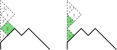
Figure 31. Vanishing of $R_{2}$ in $h_{i}(1)\psi_{\alpha}$ for the path $\alpha$ given by Figure 26 a). In the second step we already changed the content of the top half-tile from $i=5$ to $i-2p-2=-1$. Now we apply the reflection equation (2.20) to move the shaded tile $h_{1}(2)$ up and evaluate it using (6.7). The two shaded half-tiles then meet together and annihilate: $\bar{h}_{0}(1)\bar{h}_{0}(-1)=s_{0}(-a_{0})=0$.

b)  $\,i$ even and $p=\frac{i}{2}-1$. In this case, in the second step, the content of the top half-tile has to be changed from $i$ to $i-2p-2=0$. This is why we extended in (6.15) the domain of definition for $\bar{h}(u)$ and derived (6.17) and (6.18) for the case $u=0$. With these extensions the calculation of $h_{i}(1)\psi_{\alpha}$ goes the standard way.

$$h_{i}(1)\psi_{\alpha}\;=\;\;\; =\;\psi_{\alpha^{-}}\,-\,\frac{[\omega]}{[\omega+1]}\psi_{\alpha^{+0}}\,+\,\psi_{\alpha^{+1}}\,+\,R^{\prime}_{2}$$

Figure 32. The result of the transformations described in Figures 27–30 in the case $m\geq 2$. The path $\alpha$ has local minima of the same height at points $i-2p_{k}-1$, $k=1,\dots,m$, and at $i-1$. In the particular example shown here we have $i=10$, $m=2$, $p_{1}=2$ and $p_{2}=4$. The term $R^{\prime}_{2}$ in the right hand side comes in place of $\psi_{\alpha^{+2}}$ in Figure 30.

Consider now a path with $m\geq 2$ local minima preceding the minimum at $i-1$ which all have the same height $\alpha_{i-1}$ (recall that we do not care about higher preceding minima and do not allow lower ones). In this case the transformations of the third step described earlier are not enough to extract the term $\psi_{\alpha^{+2}}$ and so we continue the transformation. We explain this for the case of the path shown on Figure 32.

$$=\psi_{\alpha^{+2}}\,+\tfrac{1}{[2][3]} +\,\tfrac{[3][3+\omega]}{[5][6][\omega+1]} R^{\prime}_{2}\;=\;$$

$$=\,\psi_{\alpha^{+2}}\,+\,\frac{[\omega]}{2[\omega+1]}\,\chi_{\alpha^{+0}}\,+\,R_{3}$$

Figure 33. Extraction of $\psi_{\alpha^{+2}}$ from $R^{\prime}_{2}$ in the case $m\geq 2$.

                                                                                      $$=\,\psi_{\alpha^{+3}}\,-\,\frac{[\omega]}{2[\omega+1]}\,\chi_{\alpha^{+0}} \chi_{\alpha^{+0}}\,=\; R_{3}\,=\;$$

Figure 34. Definition of the term $\chi_{\alpha^{+0}}$ and calculation of the third step residue $R_{3}$ in the case $m=2$.

Continuation of the Step 3.  As can be seen on Figure 32, the terms $\psi_{\alpha^{-}}$, $\psi_{\alpha^{+0}}$ and $\psi_{\alpha^{+1}}$ are already fixed. The term $R^{\prime}_{2}$ displayed in Figure 33 appears in the place of $\psi_{\alpha^{+2}}$ and we now continue its transformation. To extract the term $\psi_{\alpha^{+2}}$ we increase by one the contents of the (half-)tiles in the shaded trapezium in the first equality on Figure 33. This trapezium is a composition of a rectangle and a triangle and we consecutively use (6.14) and (6.17) to increase their contents, see also Figures 20 and 24). As a result, besides $\psi_{\alpha^{+0}}$ we get two more terms whose pictures are shown in the second equality on Figure 33. Using the by now standard procedures of lowering the content of the boundary half-tile (from $i-2p_{1}-1$ to $i-2p_{2}-2$ in general, and from $5$ to $0$ in the specific example on Figure 33) and pushing up, reflecting at the boundary and evaluating the strips of tiles, we extract the third step residue $R_{3}$ from the middle picture in Figure 33. All the other terms can be reduced to the same form $\chi_{\alpha^{+0}}$. Both terms $R_{3}$ and $\chi_{\alpha^{+0}}$ are shown in Figure 34 (note that $\chi_{\alpha^{+0}}$ is composed of the same factors as $\psi_{\alpha^{+0}}$ but the contents may be different).

Step 4.  Further transformation of $R_{3}$ is identical to the calculation of $R_{2}$, see Figure 30, and the result, for the case $m=2$, is presented in Figure 34. We obtain the term $\psi_{\alpha^{+3}}$ and the term $\chi_{\alpha^{+0}}$ which cancels similar term in the preceding transformation (cf. the second line in Figure 33 and the right hand side in Figure 34).

Collecting the terms in Figures 32–34 we eventually find that for the case $m=2$ the factorised formulas (4.5) indeed satisfy the type B qKZ equations in the bulk (3.22). Consideration of the cases with $m>3$ goes along the same lines.

It lasts to check the type B boundary qKZ relation (3.24) (the boundary relation (3.3) is valid due to the same arguments used in the proof of Theorem 1). Indeed, rewriting (3.24) as

$$\bar{h}_{0}(1)\,\psi_{\alpha}\,=\,\psi_{\alpha^{-0}}\,$$

one makes the assertion obvious.

This completes the proof of Theorem 2.

Appendix A Factorised solutions for type B

A.1. Case $N=2$

Here we have two paths, $\Omega^{B}=\raisebox{0.0pt}{\includegraphics[height=20.0pt]{2_210.eps}}$ and . From the preliminary analysis we know that $\psi_{\,\includegraphics[width=8.0pt]{2_210.eps}}$ is given by (3.20) and satisfies equation

$$-a_{1}\psi_{\,\includegraphics[width=8.0pt]{2_210.eps}}\,=\,h_{1}(-1)\psi_{\,\includegraphics[width=8.0pt]{2_210.eps}}\,=\,0.$$ (A.1)

Now we may apply the boundary generator to obtain the component function $\psi_{\,\includegraphics[width=8.0pt]{2_010.eps}}$, and from (3.24) we find

$$s_{0}\psi_{\,\includegraphics[width=8.0pt]{2_210.eps}}\,=\,\psi_{\,\includegraphics[width=8.0pt]{2_010.eps}}.$$ (A.2)

Notice, that acting by $h_{1}(1)$ on $\psi_{\,\includegraphics[width=8.0pt]{2_010.eps}}$ we can get back to $\psi_{\,\includegraphics[width=8.0pt]{2_210.eps}}$, see (3.22),

$$h_{1}(1)\psi_{\,\includegraphics[width=8.0pt]{2_010.eps}}\,=\,\psi_{\,\includegraphics[width=8.0pt]{2_210.eps}},$$

which can be equivalently written as

$$h_{1}(1)\Bigl{(}s_{0}-\frac{1}{[2]}\Bigr{)}\psi_{\,\includegraphics[width=8.0pt]{2_210.eps}}\,=\,0,$$ (A.3)

where we used (A.1), (A.2) and relation (2.12). Equation (A.3) is the truncation condition to be satisfied by $\psi_{\,\includegraphics[width=8.0pt]{2_210.eps}}$.

A.2. Case $N=3$

In this case there are three paths: $\Omega^{B}=\raisebox{0.0pt}{\includegraphics[height=20.0pt]{3_3210.eps}}$, and .

As before, we start with the component function $\psi_{\Omega}^{\rm B}=\psi_{\,\includegraphics[width=12.0pt]{3_3210.eps}}$ given by (3.20) and satisfying relations

$$h_{1}(-1)\psi_{\,\includegraphics[width=12.0pt]{3_3210.eps}}\,=\,h_{2}(-1)\psi_{\,\includegraphics[width=12.0pt]{3_3210.eps}}\,=\,0.$$ (A.4)

Then we act with the boundary generator and obtain

$$s_{0}\psi_{\,\includegraphics[width=12.0pt]{3_3210.eps}}\,=\,\psi_{\,\raisebox{-4.0pt}{\smash{\includegraphics[width=12.0pt]{3_1210.eps}}}}.$$ (A.5)

Next, we apply $h_{1}(1)$ and find

$$h_{1}(1)\psi_{\,\raisebox{-4.0pt}{\smash{\includegraphics[width=12.0pt]{3_1210.eps}}}}\,=\,\psi_{\,\includegraphics[width=12.0pt]{3_3210.eps}}\,+\,\psi_{\,\raisebox{-4.0pt}{\smash{\includegraphics[width=12.0pt]{3_1010.eps}}}}.$$ (A.6)

This can be rewritten to give the following expression cf. (A.3),

$$\psi_{\,\raisebox{-4.0pt}{\smash{\includegraphics[width=12.0pt]{3_1010.eps}}}}\,=\,h_{1}(1)\Bigl{(}s_{0}-\frac{1}{[2]}\Bigr{)}\psi_{\,\includegraphics[width=12.0pt]{3_3210.eps}},$$ (A.7)

where we have used (A.4), (A.5) and (2.12). Finally, we act by operators $s_{0}$ and $h_{2}(1)$ to the rightmost term in (A.6) and obtain

$$s_{0}\psi_{\,\raisebox{-4.0pt}{\smash{\includegraphics[width=12.0pt]{3_1010.eps}}}} =\,0,$$

$$h_{2}(1)\psi_{\,\raisebox{-4.0pt}{\smash{\includegraphics[width=12.0pt]{3_1010.eps}}}} =\,\psi_{\,\raisebox{-4.0pt}{\smash{\includegraphics[width=12.0pt]{3_1210.eps}}}}\,-\,\tfrac{[\omega]}{[\omega+1]}\psi_{\,\includegraphics[width=12.0pt]{3_3210.eps}}.$$

The latter relations can be rewritten as the truncation conditions on $\psi_{\,\includegraphics[width=12.0pt]{3_3210.eps}}$:

$$s_{0}h_{1}(2)\Bigl{(}s_{0}-\tfrac{[\omega+2]}{[3][\omega+1]}\Bigr{)}\psi_{\,\includegraphics[width=12.0pt]{3_3210.eps}} =\,0,$$ (A.8)

$$h_{2}(1)h_{1}(2)\Bigl{(}s_{0}-\tfrac{[\omega+2]}{[3][\omega+1]}\Bigr{)}\psi_{\,\includegraphics[width=12.0pt]{3_3210.eps}} =\,0,$$

where we used (A.4), (A.5), (A.6) and, again, (2.12) to find factorised expressions.

Analysing the factorised expressions for the component functions in the cases $N=2,3$ we see that a proper definition for the dashed boundary half-tile is

$$\raisebox{-18.0pt}{\includegraphics[height=36.0pt]{h0.eps}}\,=\,\bar{h}_{0}(k)\,:=\,h_{0}(k)|_{\nu=\omega+p_{k}}\,=\,s_{0}\,-\,\frac{\left[\lfloor{k/2}\rfloor\right]\left[\omega+\lfloor{(k+1)/2}\rfloor\right]}{[k][\omega+1]},$$

where $p_{k}=k\mbox{~{}mod 2}$. Note that the Baxterised boundary element ${\bar{h}}_{0}(u)$ is defined for integer values of its spectral parameter $u\in{\mathbb{Z}}$ as only such values appear in our considerations.

Using this notation, the expressions for the coefficients $\psi_{\alpha}$ and the truncation conditions take a simple form. For example, formulas (A.5), (A.7), (A.8) read

$$\psi_{\,\raisebox{-4.0pt}{\smash{\includegraphics[width=12.0pt]{3_1210.eps}}}}=\bar{h}_{0}(1)\psi_{\,\includegraphics[width=12.0pt]{3_3210.eps}},\qquad\psi_{\,\raisebox{-4.0pt}{\smash{\includegraphics[width=12.0pt]{3_1010.eps}}}}=h_{1}(1)\bar{h}_{0}(2)\psi_{\,\includegraphics[width=12.0pt]{3_3210.eps}},\qquad\bar{h}_{0}(1)h_{1}(2)\bar{h}_{0}(3)\psi_{\,\includegraphics[width=12.0pt]{3_3210.eps}}=0.$$

Appendix B Type A solutions

Using the factorised expressions of Theorem 1, we have computed polynomial solutions of the qKZ equation for type A from Proposition 4 in the limit $x_{i}\rightarrow 0$ up to $N=10$. These solutions are, surprisingly, polynomials in $\tau^{2}$ with positive coefficients, up to an overall factor which is a power of $\tau$. The complete solution is determined up to an overall normalisation we have chosen so that

$$\psi^{\rm A}_{\Omega}=\tau^{\lfloor N/2\rfloor(\lfloor N/2\rfloor-1)/2}.$$

Let $\alpha=(\alpha_{0},\alpha_{1},\ldots,\alpha_{N})\in\mathcal{D}_{N,p}$ be a Dyck path of length $N$ whose minima lie on or above height $\tilde{p}-1$. Then we define $c_{\alpha,p}$ as the signed sum of boxes between $\alpha$ and $\Omega(N,p)$, where the boxes at height $\tilde{p}+h$ are assigned $(-1)^{h}$. An example is given in the main text in Figure 10. The explicit expression for $c_{\alpha,p}$ is given by

$$c_{\alpha,p}=\frac{(-1)^{\tilde{p}+1}}{2}\left(\sum_{i=1}^{\lfloor N/2\rfloor}(\alpha_{2i}-\Omega_{2i}(N,p))-\sum_{i=0}^{\lfloor(N-1)/2\rfloor}(\alpha_{2i+1}-\Omega_{2i+1}(N,p))\right).$$

We furthermore define the subset $\mathcal{D}_{N,p}$ of Dyck paths of length $N$ whose local minima lie on or above height $\tilde{p}=\lfloor(N-1)/2\rfloor-p$, i.e.

$$\mathcal{D}_{N,p}=\left\{\alpha\in\mathcal{D}_{N}|\ \alpha_{i}\geq\min(\Omega_{i},\tilde{p})\right\}.$$

These definitions allow us to define the partial sums

$$S_{\pm}(N,p)=\sum_{\alpha\in\mathcal{D}_{N,p}}\tau^{\pm c_{\alpha,p}}\psi_{\alpha},$$

for which we formulate some conjectures in the main text.

B.1. $N=4$

$$\begin{array}[]{c|lc}\alpha&\psi_{\alpha}&\tau^{\pm c_{\alpha,1}}\\ \hline\cr\includegraphics[width=24.0pt]{4_01010.eps}&1+\tau^{2}&1\\ \includegraphics[width=24.0pt]{4_01210.eps}&\tau&\tau^{\pm 1}\end{array}$$

$$\begin{array}[]{ll}S_{-}(4,0)=\tau&S_{+}(4,0)=\tau\\ S_{-}(4,1)=2+\tau^{2}&S_{+}(4,1)=1+2\tau^{2}\end{array}$$

B.2. $N=5$

$$\begin{array}[]{c|lcc}\alpha&\psi_{\alpha}&\tau^{\pm c_{\alpha,2}}&\tau^{\pm c_{\alpha,1}}\\ \hline\cr\includegraphics[width=30.0pt]{5_010101.eps}&\tau^{2}(2+\tau^{2})&1&\\ \includegraphics[width=30.0pt]{5_012101.eps}&\tau^{3}&\tau^{\pm 1}&\\ \includegraphics[width=30.0pt]{5_010121.eps}&\tau(2+\tau^{2})&\tau^{\pm 1}&\\ \includegraphics[width=30.0pt]{5_012121.eps}&1+2\tau^{2}&\tau^{\pm 2}&1\\ \includegraphics[width=30.0pt]{5_012321.eps}&\tau&\tau^{\pm 1}&\tau^{\pm 1}\end{array}$$

$$\begin{array}[]{ll}S_{-}(5,0)=\tau&S_{+}(5,0)=\tau\\ S_{-}(5,1)=2(1+\tau^{2})&S_{+}(5,1)=1+3\tau^{2}\\ S_{-}(5,2)=\tau^{-2}(1+5\tau^{2}+4\tau^{4}+\tau^{6})&S_{+}(5,2)=\tau^{2}(6+5\tau^{2})\end{array}$$

B.3. $N=6$

$$\begin{array}[]{c|lcc}\alpha&\psi_{\alpha}&\tau^{\pm c_{\alpha,2}}&\tau^{\pm c_{\alpha,1}}\\ \hline\cr\includegraphics[width=36.0pt]{6_0101010.eps}&1+5\tau^{2}+4\tau^{4}+\tau^{6}&1&\\ \includegraphics[width=36.0pt]{6_0121010.eps}&\tau(2+2\tau^{2}+\tau^{4})&\tau^{\pm 1}&\\ \includegraphics[width=36.0pt]{6_0101210.eps}&\tau(1+3\tau^{2}+\tau^{4})&\tau^{\pm 1}&\\ \includegraphics[width=36.0pt]{6_0121210.eps}&2\tau^{2}(1+\tau^{2})&\tau^{\pm 2}&1\\ \includegraphics[width=36.0pt]{6_0123210.eps}&\tau^{3}&\tau^{\pm 1}&\tau^{\pm 1}\end{array}$$

$$\begin{array}[]{ll}S_{-}(6,0)=\tau^{3}&S_{+}(6,0)=\tau^{3}\\ S_{-}(6,1)=\tau^{2}(3+2\tau^{2})&S_{+}(6,1)=\tau^{2}(2+3\tau^{2})\\ S_{-}(6,2)=6+13\tau^{2}+6\tau^{4}+\tau^{6}&S_{+}(6,2)=1+8\tau^{2}+12\tau^{4}+5\tau^{6}\end{array}$$

From now on we abbreviate polynomials of the form $P(\tau)=\tau^{p}\sum_{k=0}^{r}a_{k}\tau^{2k}$ by

$$P(\tau)=\tau^{p}(a_{0},a_{1},\ldots,a_{r}).$$

For example,

$$6\tau^{2}+13\tau^{4}+6\tau^{6}+\tau^{8}\equiv\tau^{2}(6,13,6,1)$$

B.4. $N=7$

$$\begin{array}[]{c|lccc}\alpha&\psi_{\alpha}&\tau^{\pm c_{\alpha,3}}&\tau^{\pm c_{\alpha,2}}&\tau^{\pm c_{\alpha,1}}\\ \hline\cr\includegraphics[width=42.0pt]{7_01010101.eps}&\tau^{3}(6,13,6,1)&1\\ \includegraphics[width=42.0pt]{7_01210101.eps}&\tau^{4}(5,4,1)&\tau^{\pm 1}\\ \includegraphics[width=42.0pt]{7_01012101.eps}&\tau^{4}(3,4,1)&\tau^{\pm 1}\\ \includegraphics[width=42.0pt]{7_01010121.eps}&\tau^{2}(6,13,6,1)&\tau^{\pm 1}\\ \includegraphics[width=42.0pt]{7_01212101.eps}&\tau^{5}(3,2)&\tau^{\pm 2}\\ \includegraphics[width=42.0pt]{7_01232101.eps}&\tau^{6}&\tau^{\pm 1}\\ \includegraphics[width=42.0pt]{7_01210121.eps}&\tau^{3}(5,3,1)&\tau^{\pm 2}\\ \includegraphics[width=42.0pt]{7_01012121.eps}&\tau(3,11,10,2)&\tau^{\pm 2}\\ \includegraphics[width=42.0pt]{7_01012321.eps}&\tau^{2}(3,5,1)&\tau^{\pm 1}\\ \includegraphics[width=42.0pt]{7_01212121.eps}&(1,8,12,5)&\tau^{\pm 3}&1\\ \includegraphics[width=42.0pt]{7_01232121.eps}&\tau(2,3,3)&\tau^{\pm 2}&\tau^{\pm 1}\\ \includegraphics[width=42.0pt]{7_01212321.eps}&\tau(1,6,3)&\tau^{\pm 2}&\tau^{\pm 1}\\ \includegraphics[width=42.0pt]{7_01232321.eps}&\tau^{2}(2,3)&\tau^{\pm 1}&\tau^{\pm 2}&1\\ \includegraphics[width=42.0pt]{7_01234321.eps}&\tau^{3}&\tau^{\pm 2}&\tau^{\pm 1}&\tau^{\pm 1}\end{array}$$

$$\begin{array}[]{ll}S_{-}(7,0)=\tau^{3}&S_{+}(7,0)=\tau^{3}\\ S_{-}(7,1)=\tau^{2}(3,3)&S_{+}(7,1)=\tau^{2}(2,4)\\ S_{-}(7,2)=(6,21,18,5)&S_{+}(7,2)=(1,11,24,14)\\ S_{-}(7,3)=\tau^{-3}(1,14,49,62,34,9,1)&S_{+}(7,3)=\tau^{3}(24,76,56,14)\end{array}$$

B.5. $N=8$

$$\begin{array}[]{c|lccc}\alpha&\psi_{\alpha}&\tau^{\pm c_{\alpha,3}}&\tau^{\pm c_{\alpha,2}}&\tau^{\pm c_{\alpha,1}}\\ \hline\cr\includegraphics[width=48.0pt]{8_010101010.eps}&(1,14,49,62,34,9,1)&1\\ \includegraphics[width=48.0pt]{8_012101010.eps}&\tau(3,15,29,20,7,1)&\tau^{\pm 1}\\ \includegraphics[width=48.0pt]{8_010121010.eps}&\tau(2,15,27,19,7,1)&\tau^{\pm 1}\\ \includegraphics[width=48.0pt]{8_010101210.eps}&\tau(1,12,28,25,8,1)&\tau^{\pm 1}\\ \includegraphics[width=48.0pt]{8_012121010.eps}&\tau^{2}(6,21,18,9,2)&\tau^{\pm 2}\\ \includegraphics[width=48.0pt]{8_012321010.eps}&\tau^{3}(5,5,3,1)&\tau^{\pm 1}\\ \includegraphics[width=48.0pt]{8_012101210.eps}&\tau^{2}(3,9,12,5,1)&\tau^{\pm 2}\\ \includegraphics[width=48.0pt]{8_010121210.eps}&\tau^{2}(2,15,24,13,2)&\tau^{\pm 2}\\ \includegraphics[width=48.0pt]{8_010123210.eps}&\tau^{3}(1,6,6,1)&\tau^{\pm 1}\\ \includegraphics[width=48.0pt]{8_012121210.eps}&\tau^{3}(6,21,18,5)&\tau^{\pm 3}&1\\ \includegraphics[width=48.0pt]{8_012321210.eps}&\tau^{4}(5,6,3)&\tau^{\pm 2}&\tau^{\pm 1}\\ \includegraphics[width=48.0pt]{8_012123210.eps}&\tau^{4}(3,8,3)&\tau^{\pm 2}&\tau^{\pm 1}\\ \includegraphics[width=48.0pt]{8_012323210.eps}&\tau^{5}(3,3)&\tau^{\pm 1}&\tau^{\pm 2}&1\\ \includegraphics[width=48.0pt]{8_012343210.eps}&\tau^{6}&\tau^{\pm 2}&\tau^{\pm 1}&\tau^{\pm 1}\end{array}$$

$$\begin{array}[]{ll}S_{-}(8,0)=\tau^{6}&S_{+}(8,0)=\tau^{6}\\ S_{-}(8,1)=\tau^{5}(4,3)&S_{+}(8,1)=\tau^{5}(3,4)\\ S_{-}(8,2)=\tau^{3}(17,39,24,5)&S_{+}(8,2)=\tau^{3}(6,29,36,14)\\ S_{-}(8,3)=(24,136,234,176,63,12,1)&S_{+}(8,3)=(1,20,108,219,200,84,14)\end{array}$$

B.6. $N=9$

$$\begin{array}[]{c|lc}\alpha&\psi_{\alpha}&\tau^{\pm c_{\alpha,4}}\\ \hline\cr\includegraphics[width=54.0pt]{9_0101010101.eps}&\tau^{4}(24,136,234,176,63,12,1)&1\\ \includegraphics[width=54.0pt]{9_0121010101.eps}&\tau^{5}(28,84,94,43,10,1)&\tau^{\pm 1}\\ \includegraphics[width=54.0pt]{9_0101210101.eps}&\tau^{5}(20,72,84,41,10,1)&\tau^{\pm 1}\\ \includegraphics[width=54.0pt]{9_0101012101.eps}&\tau^{5}(12,58,74,41,10,1)&\tau^{\pm 1}\\ \includegraphics[width=54.0pt]{9_0101010121.eps}&\tau^{3}(24,136,234,176,63,12,1)&\tau^{\pm 1}\\ \includegraphics[width=54.0pt]{9_0121210101.eps}&\tau^{6}(28,65,45,15,2)&\tau^{\pm 2}\\ \includegraphics[width=54.0pt]{9_0121012101.eps}&\tau^{6}(14,31,23,7,1)&\tau^{\pm 2}\\ \includegraphics[width=54.0pt]{9_0121010121.eps}&\tau^{4}(28,84,90,40,10,1)&\tau^{\pm 2}\\ \includegraphics[width=54.0pt]{9_0101212101.eps}&\tau^{6}(12,41,41,16,2)&\tau^{\pm 2}\\ \includegraphics[width=54.0pt]{9_0101210121.eps}&\tau^{4}(20,68,74,34,9,1)&\tau^{\pm 2}\\ \includegraphics[width=54.0pt]{9_0101012121.eps}&\tau^{2}(12,86,208,213,103,22,2)&\tau^{\pm 2}\\ \includegraphics[width=54.0pt]{9_0123210101.eps}&\tau^{7}(14,13,6,1)&\tau^{\pm 1}\\ \includegraphics[width=54.0pt]{9_0101232101.eps}&\tau^{7}(4,10,7,1)&\tau^{\pm 1}\\ \includegraphics[width=54.0pt]{9_0101012321.eps}&\tau^{3}(12,62,88,51,11,1)&\tau^{\pm 1}\end{array}$$

$$\begin{array}[]{c|lc}\alpha&\psi_{\alpha}&\tau^{\pm c_{\alpha,4}}\\ \hline\cr\includegraphics[width=54.0pt]{9_0121212101.eps}&\tau^{7}(17,39,24,5)&\tau^{\pm 3}\\ \includegraphics[width=54.0pt]{9_0121210121.eps}&\tau^{5}(28,59,33,12,2)&\tau^{\pm 3}\\ \includegraphics[width=54.0pt]{9_0121012121.eps}&\tau^{3}(14,56,84,54,15,2)&\tau^{\pm 3}\\ \includegraphics[width=54.0pt]{9_0101212121.eps}&\tau(4,46,160,230,154,47,5)&\tau^{\pm 3}\\ \includegraphics[width=54.0pt]{9_0123212101.eps}&\tau^{8}(9,9,3)&\tau^{\pm 2}\\ \includegraphics[width=54.0pt]{9_0121232101.eps}&\tau^{8}(6,10,3)&\tau^{\pm 2}\\ \includegraphics[width=54.0pt]{9_0123232101.eps}&\tau^{9}(4,3)&\tau^{\pm 1}\\ \includegraphics[width=54.0pt]{9_0123432101.eps}&\tau^{10}&\tau^{\pm 2}\\ \includegraphics[width=54.0pt]{9_0123210121.eps}&\tau^{6}(14,9,4,1)&\tau^{\pm 2}\\ \includegraphics[width=54.0pt]{9_0121012321.eps}&\tau^{4}(14,28,25,7,1)&\tau^{\pm 2}\\ \includegraphics[width=54.0pt]{9_0101232121.eps}&\tau^{2}(8,40,68,61,26,3)&\tau^{\pm 2}\\ \includegraphics[width=54.0pt]{9_0101212321.eps}&\tau^{2}(4,38,96,84,28,3)&\tau^{\pm 2}\\ \includegraphics[width=54.0pt]{9_0101232321.eps}&\tau^{3}(8,40,56,27,3)&\tau^{\pm 1}\\ \includegraphics[width=54.0pt]{9_0101234321.eps}&\tau^{4}(4,14,9,1)&\tau^{\pm 2}\end{array}$$

$$\begin{array}[]{c|lcccc}\alpha&\psi_{\alpha}&\tau^{\pm c_{\alpha,4}}&\tau^{\pm c_{\alpha,3}}&\tau^{\pm c_{\alpha,2}}&\tau^{\pm c_{\alpha,1}}\\ \hline\cr\includegraphics[width=54.0pt]{9_0121212121.eps}&(1,20,108,219,200,84,14)&\tau^{\pm 4}&1\\ \includegraphics[width=54.0pt]{9_0123212121.eps}&\tau(3,19,58,69,38,9)&\tau^{\pm 3}&\tau^{\pm 1}\\ \includegraphics[width=54.0pt]{9_0121232121.eps}&\tau(2,27,67,75,47,10)&\tau^{\pm 3}&\tau^{\pm 1}\\ \includegraphics[width=54.0pt]{9_0121212321.eps}&\tau(1,18,75,106,51,9)&\tau^{\pm 3}&\tau^{\pm 1}\\ \includegraphics[width=54.0pt]{9_0123232121.eps}&\tau^{2}(6,29,36,30,11)&\tau^{\pm 3}&\tau^{\pm 2}\\ \includegraphics[width=54.0pt]{9_0123212321.eps}&\tau^{2}(3,13,33,21,6)&\tau^{\pm 2}&\tau^{\pm 2}\\ \includegraphics[width=54.0pt]{9_0121232321.eps}&\tau^{2}(2,27,64,51,11)&\tau^{\pm 2}&\tau^{\pm 2}\\ \includegraphics[width=54.0pt]{9_0123432121.eps}&\tau^{3}(5,7,6,4)&\tau^{\pm 3}&\tau^{\pm 1}\\ \includegraphics[width=54.0pt]{9_0121234321.eps}&\tau^{3}(1,12,17,4)&\tau^{\pm 3}&\tau^{\pm 1}\\ \includegraphics[width=54.0pt]{9_0123232321.eps}&\tau^{3}(6,29,36,14)&\tau^{\pm 1}&\tau^{\pm 3}&1\\ \includegraphics[width=54.0pt]{9_0123432321.eps}&\tau^{4}(5,8,6)&\tau^{\pm 2}&\tau^{\pm 2}&\tau^{\pm 1}\\ \includegraphics[width=54.0pt]{9_0123234321.eps}&\tau^{4}(3,12,6)&\tau^{\pm 2}&\tau^{\pm 2}&\tau^{\pm 1}\\ \includegraphics[width=54.0pt]{9_0123434321.eps}&\tau^{5}(3,4)&\tau^{\pm 3}&\tau^{\pm 1}&\tau^{\pm 2}&1\\ \includegraphics[width=54.0pt]{9_0123454321.eps}&\tau^{6}&\tau^{\pm 2}&\tau^{\pm 2}&\tau^{\pm 1}&\tau^{\pm 1}\\ \end{array}$$

$$S_{-}(9,0) =\tau^{6}$$

$$S_{-}(9,1) =\tau^{5}(4,4)$$

$$S_{-}(9,2) =\tau^{3}(17,54,48,14)$$

$$S_{-}(9,3) =(24,196,520,624,372,112,14)$$

$$S_{-}(9,4) =\tau^{-4}(1,30,273,1042,2006,2121,1321,501,117,16)$$

$$S_{+}(0,0) =\tau^{6}$$

$$S_{+}(9,1) =\tau^{5}(3,5)$$

$$S_{+}(9,2) =\tau^{3}(6,37,60,30)$$

$$S_{+}(9,3) =(1,26,189,524,660,378,84)$$

$$S_{+}(9,4) =\tau^{4}(120,920,2242,2440,1305,360,42)$$

B.6.1. $N=10$

$$\begin{array}[]{c|lc}\alpha&\psi_{\alpha}&\tau^{\pm c_{\alpha,4}}\\ \hline\cr\includegraphics[width=54.0pt]{10_01010101010.eps}&(1,30,273,1042,2006,2121,1321,501,117,16,1)&1\\ \includegraphics[width=54.0pt]{10_01210101010.eps}&\tau(4,56,294,738,977,735,327,89,14,1)&\tau^{\pm 1}\\ \includegraphics[width=54.0pt]{10_01012101010.eps}&\tau(3,49,269,683,912,691,312,87,14,1)&\tau^{\pm 1}\\ \includegraphics[width=54.0pt]{10_01010121010.eps}&\tau(2,47,267,686,915,688,313,88,14,1)&\tau^{\pm 1}\\ \includegraphics[width=54.0pt]{10_01010101210.eps}&\tau(1,28,220,669,996,820,384,101,15,1)&\tau^{\pm 1}\\ \includegraphics[width=54.0pt]{10_01212101010.eps}&\tau^{2}(12,116,396,684,348,117,23,2)&\tau^{\pm 2}\\ \includegraphics[width=54.0pt]{10_01210121010.eps}&\tau^{2}(8,60,206,350,329,176,58,11,1)&\tau^{\pm 2}\\ \includegraphics[width=54.0pt]{10_01210101210.eps}&\tau^{2}(4,48,210,394,403,230,72,13,1)&\tau^{\pm 2}\\ \includegraphics[width=54.0pt]{10_01012121010.eps}&\tau^{2}(6,89,368,665,618,342,120,24,2)&\tau^{\pm 2}\\ \includegraphics[width=54.0pt]{10_01012101210.eps}&\tau^{2}(3,43,184,343,349,200,64,12,1)&\tau^{\pm 2}\\ \includegraphics[width=54.0pt]{10_01010121210.eps}&\tau^{2}(2,47,264,632,744,469,159,27,2)&\tau^{\pm 2}\\ \includegraphics[width=54.0pt]{10_01232101010.eps}&\tau^{3}(14,70,151,180,111,43,10,1)&\tau^{\pm 1}\\ \includegraphics[width=54.0pt]{10_01012321010.eps}&\tau^{3}(5,57,156,174,111,46,11,1)&\tau^{\pm 1}\\ \includegraphics[width=54.0pt]{10_01010123210.eps}&\tau^{3}(1,22,102,97,172,72,13,1)&\tau^{\pm 1}\end{array}$$

$$\begin{array}[]{c|lc}\alpha&\psi_{\alpha}&\tau^{\pm c_{\alpha,4}}\\ \hline\cr\includegraphics[width=54.0pt]{10_01212121010.eps}&\tau^{3}(24,196,520,624,408,174,44,5)&\tau^{\pm 3}\\ \includegraphics[width=54.0pt]{10_01212101210.eps}&\tau^{3}(12,92,216,276,198,76,18,2)&\tau^{\pm 3}\\ \includegraphics[width=54.0pt]{10_01210121210.eps}&\tau^{3}(8,60,194,286,226,94,20,2)&\tau^{\pm 3}\\ \includegraphics[width=54.0pt]{10_01012121210.eps}&\tau^{3}(6,89,368,649,564,256,58,5)&\tau^{\pm 3}\\ \includegraphics[width=54.0pt]{10_01232121010.eps}&\tau^{4}(28,112,187,140,69,21,3)&\tau^{\pm 2}\\ \includegraphics[width=54.0pt]{10_01212321010.eps}&\tau^{4}(20,118,189,142,71,22,3)&\tau^{\pm 2}\\ \includegraphics[width=54.0pt]{10_01232321010.eps}&\tau^{5}(28,84,73,42,16,3)&\tau^{\pm 1}\\ \includegraphics[width=54.0pt]{10_01234321010.eps}&\tau^{6}(14,14,9,4,1)&\tau^{\pm 2}\\ \includegraphics[width=54.0pt]{10_01232101210.eps}&\tau^{4}(14,42,64,57,25,7,1)&\tau^{\pm 2}\\ \includegraphics[width=54.0pt]{10_01210123210.eps}&\tau^{4}(4,24,63,70,39,9,1)&\tau^{\pm 2}\\ \includegraphics[width=54.0pt]{10_01012321210.eps}&\tau^{4}(5,58,166,190,111,32,3)&\tau^{\pm 2}\\ \includegraphics[width=54.0pt]{10_01012123210.eps}&\tau^{4}(3,42,147,206,126,33,3)&\tau^{\pm 2}\\ \includegraphics[width=54.0pt]{10_01012323210.eps}&\tau^{5}(3,34,90,85,31,3)&\tau^{\pm 1}\\ \includegraphics[width=54.0pt]{10_01012343210.eps}&\tau^{6}(1,10,20,10,1)&\tau^{\pm 2}\end{array}$$

$$\begin{array}[]{c|lccccc}\alpha&\psi_{\alpha}&\tau^{\pm c_{\alpha,4}}&\tau^{\pm c_{\alpha,3}}&\tau^{\pm c_{\alpha,2}}&\tau^{\pm c_{\alpha,1}}\\ \hline\cr\includegraphics[width=54.0pt]{10_01212121210.eps}&\tau^{4}(24,196,520,6224,372,112,14)&\tau^{\pm 4}&1\\ \includegraphics[width=54.0pt]{10_01232121210.eps}&\tau^{5}(28,112,191,144,55,9)&\tau^{\pm 3}&\tau^{\pm 1}\\ \includegraphics[width=54.0pt]{10_01212321210.eps}&\tau^{5}(20,122,209,162,165,10)&\tau^{\pm 3}&\tau^{\pm 1}\\ \includegraphics[width=54.0pt]{10_01212123210.eps}&\tau^{5}(12,88,192,174,64,9)&\tau^{\pm 3}&\tau^{\pm 1}\\ \includegraphics[width=54.0pt]{10_01232321210.eps}&\tau^{6}(28,90,80,48,11)&\tau^{\pm 3}&\tau^{\pm 2}\\ \includegraphics[width=54.0pt]{10_01232123210.eps}&\tau^{6}(14,45,60,29,6)&\tau^{\pm 2}&\tau^{\pm 2}\\ \includegraphics[width=54.0pt]{10_01212323210.eps}&\tau^{6}(12,71,110,63,11)&\tau^{\pm 2}&\tau^{\pm 2}\\ \includegraphics[width=54.0pt]{10_01234321210.eps}&\tau^{7}(14,18,12,4)&\tau^{\pm 3}&\tau^{\pm 1}\\ \includegraphics[width=54.0pt]{10_01212343210.eps}&\tau^{7}(4,20,20,4)&\tau^{\pm 3}&\tau^{\pm 1}\\ \includegraphics[width=54.0pt]{10_01232323210.eps}&\tau^{7}(17,54,48,14)&\tau^{\pm 1}&\tau^{\pm 3}&1\\ \includegraphics[width=54.0pt]{10_01234323210.eps}&\tau^{8}(9,12,6)&\tau^{\pm 2}&\tau^{\pm 2}&\tau^{\pm 1}\\ \includegraphics[width=54.0pt]{10_01232343210.eps}&\tau^{8}(6,15,6)&\tau^{\pm 2}&\tau^{\pm 2}&\tau^{\pm 1}\\ \includegraphics[width=54.0pt]{10_01234343210.eps}&\tau^{9}(4,4)&\tau^{\pm 3}&\tau^{\pm 1}&\tau^{\pm 2}&1\\ \includegraphics[width=54.0pt]{10_01234543210.eps}&\tau^{10}&\tau^{\pm 2}&\tau^{\pm 2}&\tau^{\pm 1}&\tau^{\pm 1}\\ \end{array}$$

$$S_{-}(10,0) =\tau^{10}$$

$$S_{-}(10,1) =\tau^{9}(5,4)$$

$$S_{-}(10,2) =\tau^{7}(36,86,60,14)$$

$$S_{-}(10,3) =\tau^{4}(155,811,1490,1306,592,140,14)$$

$$S_{-}(10,4) =(120,1400,5754,11584,13071,8900,3805,1044,186,20,1)$$

$$S_{+}(10,0) =\tau^{10}$$

$$S_{+}(10,1) =\tau^{9}(4,5)$$

$$S_{+}(10,2) =\tau^{7}(17,69,80,30)$$

$$S_{+}(10,3) =\tau^{4}(24,256,914,1496,1230,504,84)$$

$$S_{+}(10,4) =(1,40,508,2799,7940,12652,12026,6967,2430,480,42)$$

Appendix C Type B solutions

Using the factorised expressions of Theorem 2, we have computed polynomial solutions of the qKZ equation for type B from Proposition 6 in the limit $x_{i}\rightarrow 0$ up to $N=6$. In the following variables,

$$\tau^{\prime 2}=2-\tau=2+[2]=[2]_{q^{1/2}}^{2},\qquad a=-\left.\frac{[\omega+1]}{[\frac{\omega-\delta}{2}][\frac{\omega+\delta}{2}]}\right|_{\omega=-1/2},$$

see also Remark 1, and up to an overall normalisation, these solutions become polynomials with positive coefficients. We choose the normalisation such that

$$\psi_{\Omega}^{\rm B}=a^{\lfloor N/2\rfloor}.$$

C.1. $N=2$

$$\begin{array}[]{c|l}\alpha&\psi_{\alpha}\\ \hline\cr\includegraphics[width=12.0pt]{2_010.eps}&1\\ \includegraphics[width=12.0pt]{2_210.eps}&a\end{array}$$

C.2. $N=3$

$$\begin{array}[]{c|l}\alpha&\psi_{\alpha}\\ \hline\cr\includegraphics[width=18.0pt]{3_1010.eps}&1+\tau^{\prime 2}+a\\ \includegraphics[width=18.0pt]{3_1210.eps}&2\\ \includegraphics[width=18.0pt]{3_3210.eps}&a\end{array}$$

C.3. $N=4$

$$\begin{array}[]{c|l}\alpha&\psi_{\alpha}\\ \hline\cr\includegraphics[width=24.0pt]{4_01010.eps}&5+\tau^{\prime 2}+a(2+\tau^{\prime 2})\\ \includegraphics[width=24.0pt]{4_21010.eps}&a(3+2\tau^{\prime 2}+\tau^{\prime 4})+a^{2}(2+\tau^{\prime 2})\\ \includegraphics[width=24.0pt]{4_01210.eps}&2+\tau^{\prime 2}\\ \includegraphics[width=24.0pt]{4_21210.eps}&2a(2+\tau^{\prime 2})+2a^{2}\\ \includegraphics[width=24.0pt]{4_23210.eps}&3a\\ \includegraphics[width=24.0pt]{4_43210.eps}&a^{2}\end{array}$$

C.4. $N=5$

$$\begin{array}[]{c|l}\alpha&\psi_{\alpha}\\ \hline\cr\includegraphics[width=30.0pt]{5_101010.eps}&9+17\tau^{\prime 2}+6\tau^{\prime 4}+\tau^{\prime 6}+a(16+17\tau^{\prime 2}+3\tau^{\prime 4})+a^{2}(7+2\tau^{\prime 2})\\ \includegraphics[width=30.0pt]{5_101210.eps}&2+5\tau^{\prime 2}+3\tau^{\prime 4}+\tau^{\prime 6}+a(4+6\tau^{\prime 2}+2\tau^{\prime 4})+a^{2}(2+\tau^{\prime 2})\\ \includegraphics[width=30.0pt]{5_121010.eps}&12+17\tau^{\prime 2}+4\tau^{\prime 4}+a(12+5\tau^{\prime 2}+\tau^{\prime 4})\\ \includegraphics[width=30.0pt]{5_321010.eps}&a(1+\tau^{\prime 2})(5+3\tau^{\prime 2}+\tau^{\prime 4})+a^{2}(5+3\tau^{\prime 2}+\tau^{\prime 4})\\ \includegraphics[width=30.0pt]{5_121210.eps}&24+8\tau^{\prime 2}+\tau^{\prime 4}+a(8+3\tau^{\prime 2})\\ \includegraphics[width=30.0pt]{5_321210.eps}&a(12+7\tau^{\prime 2}+2\tau^{\prime 4})+2a^{2}(3+\tau^{\prime 2})\\ \includegraphics[width=30.0pt]{5_123210.eps}&8+3\tau^{\prime 2}\\ \includegraphics[width=30.0pt]{5_323210.eps}&3a(3+\tau^{\prime 2})+3a^{2}\\ \includegraphics[width=30.0pt]{5_343210.eps}&4a\\ \includegraphics[width=30.0pt]{5_543210.eps}&a^{2}\end{array}$$

C.5. $N=6$

$$\begin{array}[]{c|l}\alpha&\psi_{\alpha}\\ \hline\cr\includegraphics[width=36.0pt]{6_0101010.eps}&149+107\tau^{\prime 2}+27\tau^{\prime 4}+3\tau^{\prime 6}+a(126+131\tau^{\prime 2}+45\tau^{\prime 4}+9\tau^{\prime 6}+\tau^{\prime 8})\\ &+a^{2}(32+36\tau^{\prime 2}+9\tau^{\prime 4}+\tau^{\prime 6})\\ \includegraphics[width=36.0pt]{6_0101210.eps}&58+57\tau^{\prime 2}+14\tau^{\prime 4}+\tau^{\prime 6}+a(32+44\tau^{\prime 2}+21\tau^{\prime 4}+6\tau^{\prime 6}+\tau^{\prime 8})\\ &+a^{2}(1+\tau^{\prime 2})(8+4\tau^{\prime 2}+\tau^{\prime 4})\\ \includegraphics[width=36.0pt]{6_0121010.eps}&52+50\tau^{\prime 2}+21\tau^{\prime 4}+6\tau^{\prime 6}+\tau^{\prime 8}+a(32+36\tau^{\prime 2}+9\tau^{\prime 4}+\tau^{\prime 6})\\ \includegraphics[width=36.0pt]{6_0121210.eps}&2(20+24\tau^{\prime 2}+7\tau^{\prime 4}+\tau^{\prime 6})+a(1+\tau^{\prime 2})(8+4\tau^{\prime 2}+\tau^{\prime 4})\\ \includegraphics[width=36.0pt]{6_0123210.eps}&(1+\tau^{\prime 2})(8+4\tau^{\prime 2}+\tau^{\prime 4})\\ \includegraphics[width=36.0pt]{6_2101010.eps}&a(81+101\tau^{\prime 2}+70\tau^{\prime 4}+26\tau^{\prime 6}+7\tau^{\prime 8}+\tau^{\prime 10})+a^{2}(94+127\tau^{\prime 2}+72\tau^{\prime 4}+17\tau^{\prime 6}+2\tau^{\prime 8})\\ &+a^{3}(32+36\tau^{\prime 2}+9\tau^{\prime 4}+\tau^{\prime 6})\\ \includegraphics[width=36.0pt]{6_2101210.eps}&a(26+37\tau^{\prime 2}+25\tau^{\prime 4}+11\tau^{\prime 6}+4\tau^{\prime 8}+\tau^{\prime 1}0)+a^{2}(12+20\tau^{\prime 2}+14\tau^{\prime 4}+5\tau^{\prime 6}+\tau^{\prime 8})\\ &+a^{3}(1+\tau^{\prime 2})(8+4\tau^{\prime 2}+\tau^{\prime 4})\\ \includegraphics[width=36.0pt]{6_2121010.eps}&a(72+104\tau^{\prime 2}+81\tau^{\prime 4}+25\tau^{\prime 6}+4\tau^{\prime 8})+a^{2}(84+107\tau^{\prime 2}+55\tau^{\prime 4}+9\tau^{\prime 6})\\ &+a^{3}(2+\tau^{\prime 2})(12+5\tau^{\prime 2})\\ \includegraphics[width=36.0pt]{6_2321010.eps}&a(39+58\tau^{\prime 2}+49\tau^{\prime 4}+10\tau^{\prime 6})+a^{2}(2+\tau^{\prime 2})(17+8\tau^{\prime 2}+\tau^{\prime 4})\\ \includegraphics[width=36.0pt]{6_4321010.eps}&a^{2}(11+19\tau^{\prime 2}+19\tau^{\prime 4}+7\tau^{\prime 6}+\tau^{\prime 8})+a^{3}(2+\tau^{\prime 2})(5+3\tau^{\prime 2}+\tau^{\prime 4})\\ \includegraphics[width=36.0pt]{6_2121210.eps}&a(104+128\tau^{\prime 2}+44\tau^{\prime 4}+9\tau^{\prime 6}+\tau^{\prime 8})+a^{2}(104+92\tau^{\prime 2}+22\tau^{\prime 4}+2\tau^{\prime 6})\\ &+a^{3}(32+11\tau^{\prime 2}+\tau^{\prime 4})\\ \includegraphics[width=36.0pt]{6_2123210.eps}&3a(1+\tau^{\prime 2})(8+4\tau^{\prime 2}+\tau^{\prime 4})+a^{2}(3+2\tau^{\prime 2})(8+3\tau^{\prime 2})+a^{3}(14+3\tau)\\ \end{array}$$

$$\begin{array}[]{c|l}\alpha&\psi_{\alpha}\\ \hline\cr\includegraphics[width=36.0pt]{6_2321210.eps}&a(84+78\tau^{\prime 2}+19\tau^{\prime 4}+\tau^{\prime 6})+a^{2}(50+20\tau^{\prime 2}+3\tau^{\prime 4})\\ \includegraphics[width=36.0pt]{6_4321210.eps}&2a^{2}(2+\tau^{\prime 2})(7+4\tau^{\prime 2}+\tau^{\prime 4})+2a^{3}(24+6\tau^{\prime 2}+2\tau^{\prime 4})\\ \includegraphics[width=36.0pt]{6_2323210.eps}&a(75+26\tau^{\prime 2}+3\tau^{\prime 4})+2a^{2}(10+3\tau^{\prime 2})\\ \includegraphics[width=36.0pt]{6_4323210.eps}&a^{2}(31+15\tau^{\prime 2}+3\tau^{\prime 4})+3a^{3}(4+\tau^{\prime 2})\\ \includegraphics[width=36.0pt]{6_2343210.eps}&2a(10+3\tau^{\prime 2})\\ \includegraphics[width=36.0pt]{6_4343210.eps}&4a^{2}(4+\tau^{\prime 2})+4a^{3}\\ \includegraphics[width=36.0pt]{6_4543210.eps}&5a^{2}\\ \includegraphics[width=36.0pt]{6_6543210.eps}&a^{3}\end{array}$$

References

- [1] F.C. Alcaraz, P. Pyatov, and V. Rittenberg, Raise and Peel Models of fluctuating interfaces and combinatorics of Pascal’s hexagon, [arXiv:0709.4575].
- [2] M.T. Batchelor, J. de Gier and B. Nienhuis, The quantum symmetric XXZ chain at , alternating sign matrices and plane partitions, 2001 J. Phys. A 34 L265–L270, arXiv:cond-mat/0101385.
- [3] M. Beccaria and G. F. De Angelis, Exact Ground State and Finite Size Scaling in a Supersymmetric Lattice Model, Phys. Rev. Lett. 94 (2005) 100401, arXiv:cond-mat/0407752;
- [4] D. Bressoud, Proofs and confirmations. The story of the alternating sign matrix conjecture (Cambridge University Press, 1999).
- [5] I Cherednik, Double affine Hecke algebras, London Mathematical Society Lecture Notes Series 319, (Cambridge University Press, Cambridge, 2005).
- [6] J. de Gier, Loops, matchings and alternating-sign matrices, Discr. Math. 298 (2005) 365-388, arXiv:math.CO/0211285.
- [7] J. de Gier, A. Nichols, P.Pyatov and V. Rittenberg, Magic in the spectra of the XXZ quantum chain with boundaries at and , Nucl. Phys. B729 (2005) 387-418, arXiv:hep-th/0505062.
- [8] J. de Gier and B. Nienhuis, Brauer loops and the commuting variety, J. Stat. Mech. (2005) P01006, [math-ph/0410392]
- [9] J. de Gier, B. Nienhuis, P.A. Pearce and V. Rittenberg, The raise and peel model of a fluctuating interface, J. Stat. Phys. 114 (2004) 1–35, arXiv:cond-mat/0301430.
- [10] J. de Gier, B. Nienhuis, P. A. Pearce and V. Rittenberg, Stochastic processes and conformal invariance, Phys. Rev. E 67 (2003) 016101-016104, [cond-mat/0205467].
- [11] J. de Gier and V. Rittenberg, Refined Razumov-Stroganov conjectures for open boundaries, J. Stat. Mech. (2004), P09009, [math-ph/0408042]
- [12] P. Di Francesco, Boundary qKZ equation and generalized Razumov-Stroganov sum rules for open IRF models, J. Stat. Mech. (2005) P09004, arXiv:math-ph/0509011.
- [13] P. Di Francesco, Totally Symmetric Self Complementary Plane Partitions and the quantum Knizhnik-Zamolodchikov equation: a conjecture, J. Stat. Mech. (2006) P09008, arXiv:cond-mat/0607499.
- [14] P. Di Francesco, Open boundary Quantum Knizhnik-Zamolodchikov equation and the weighted enumeration of symmetric plane partitions, J. Stat. Mech. (2007) P01024, arXiv:math-ph/0611012.
- [15] P. Di Francesco and P. Zinn-Justin, Around the Razumov-Stroganov conjecture: proof of a multi-parameter sum rule, 2005 Electron. J. Combin. 12, R6, arXiv:math-ph/0410061
- [16] P. Di Francesco, P. Zinn-Justin, Inhomogeneous model of crossing loops and multidegrees of some algebraic varieties, Commun. Math. Phys. 262 (2006), 459-487, arXiv:math-ph/0412031.
- [17] P. Di Francesco and P. Zinn-Justin, Quantum Knizhnik-Zamolodchikov equation, generalized Razumov-Stroganov sum rules and extended Joseph polynomials, 2005 J. Phys. A 38, L815–L822, arXiv:math-ph/0508059.
- [18] P. Di Francesco and P. Zinn-Justin, Quantum Knizhnik-Zamolodchikov equation: reflecting boundary conditions and combinatorics, arXiv:math-ph/0709.3410
- [19] P. Di Francesco, P. Zinn-Justin and J.-B. Zuber A Bijection between classes of Fully Packed Loops and Plane Partitions, Electron. J. Combin. 11 (2004) 64, arXiv:math/0311220.
- [20] P. Di Francesco, P. Zinn-Justin and J.-B. Zuber Sum rules for the ground states of the O(1) loop model on a cylinder and the XXZ spin chain, Electron. J. Combin. 11 (2004) 64, arXiv:math-ph/0603009.
- [21] G. Duchamp, D. Krob, A. Lascoux, B. Leclerc, T. Scharf, and J.-Y. Thibon, Euler-Poincaré characteristic and polynomial representations of Iwahori-Hecke algebras, Publ. RIMS, 31 (1995) 179-201.
- [22] P.I. Etingof, I.B. Frenkel and A.A. Kirillov Jr., Lectures on representation theory and Knizhnik-Zamolodchikov equations, Mathematical Surveys and Monographs 58 (AMS, Providence, 1998).
- [23] P. Fendley, B. Nienhuis and K. Schoutens, Lattice fermion models with supersymmetry, J. Phys. A 36 (2003) 12399-12424, arXiv:cond-mat/0307338.
- [24] I.B. Frenkel and N. Reshetikhin, Quantum affine algebras and holonomic difference equations, Commun. Math. Phys. 146 (1992), 1–60.
- [25] A.P. Isaev and O.V. Ogievetsky, Baxterized Solutions of Reflection Equation and Integrable Chain Models, Nucl. Phys. B760 (2007) 167-183, arXiv:math-ph/0510078.
- [26] M. Jimbo and T. Miwa, Algebraic analysis of solvable lattice models (AMS, Providence, 1995).
- [27] V.F.R. Jones, On a certain value of the Kauffman polynomial, Comm. Math. Phys. 125 (1989) 459–467.
- [28] M. Kasatani and V. Pasquier, On polynomials interpolating between the stationary state of a O(n) model and a Q.H.E. ground state, arXiv:cond-mat/0608160.
- [29] M. Kasatani and Y. Takeyama, The quantum Knizhnik-Zamolodchikov equation and non-symmetric Macdonald polynomials, arXiv:math.CO/0608773.
- [30] A. Kirillov Jr. and A. Lascoux, Factorization of Kazhdan-Lusztig elements for Grassmanians, Adv. Stud. 28 (2000), 143–154; arXiv:math.CO/9902072.
- [31] A. Knutson, P. Zinn-Justin, A scheme related to the Brauer loop model, Adv. in Math. 214 (2007) 40-77, arXiv:math.CO/0503224.
- [32] P.P. Martin and H. Saleur, The blob algebra and the periodic Temperley-Lieb algebra, Lett. Math. Phys. 30 (1994) 189-206, arXiv:hep-th/9302094.
- [33] S. Mitra, B. Nienhuis, J. de Gier and M.T. Batchelor, Exact expressions for correlations in the ground state of the dense O(1) loop model, J. Stat. Mech. (2004) P09010 arXiv:cond-mat/0401245.
- [34] V. Pasquier, Quantum incrompressibility and Razumov Stroganov type conjectures, Ann. Henri Poincare’ 7, 397-421 (2006) arXiv:cond-mat/0506075.
- [35] P. A. Pearce, V. Rittenberg, J. de Gier and B. Nienhuis, Temperley-Lieb stochastic processes, J. Phys. A 35 (2002) L661-L668, arXiv:math-ph/0209017.
- [36] P. Pyatov, Raise and Peel Models of fluctuating interfaces and combinatorics of Pascal’s hexagon, J. Stat. Mech. (2004) P09003, arXiv:math-ph/0406025.
- [37] A.V. Razumov and Yu.G. Stroganov, Bethe roots and refined enumeration of alternating-sign matrices., J. Stat. Mech. (2006) P07004, arXiv:math-ph/0605004;
- [38] A.V. Razumov, Yu.G. Stroganov and P. Zinn-Justin, Polynomial solutions of qKZ equation and ground state of XXZ spin chain at ., arXiv:math-ph/07043542;
- [39] A.V. Razumov and Yu.G. Stroganov, Spin chains and combinatorics, 2001 J. Phys. A 34 3185–3190, arXiv:cond-mat/0012141.
- [40] A.V. Razumov and Yu.G. Stroganov, Combinatorial nature of gound state vector of O(1) loop model, 2004 Theor. Math. Phys. 138 333–337, arXiv:math.CO/0104216.
- [41] K. Shigechi and M. Uchiyama, Ak generalization of the O(1) loop model on a cylinder: Affine HeckeS algebra, -KZ equation and the sum rule, arXiv:math-ph/0612001
- [42] E. Sklyanin, Boundary conditions for integrable quantum systems, J. Phys. A 21 (1988) 2375–2489.
- [43] F.A. Smirnov, A general formula for soliton form factors in the quantum sine-Gordon model, J. Phys. A 19 (1986) L575–L578
- [44] F.A. Smirnov, Form factors in completely integrable modles of Quantum Field Theory, World Scientific, Singapore, 1992.
- [45] Yu.G. Stroganov, The importance of being odd, 2001 J. Phys. A 34 L179–L185, arXiv:cond-mat/0012035;
- [46] V. Tarasov and A. Varchenko, Jackson integrable representations for solutions of the quantized Knizhnik-Zamolodchikov equation, St.Petersburg. Math. J. 6 (1994) no.2, 275–314.
- [47] A. Varchenko, Quantized Knizhnik-Zamolodchikov equations, quantum Yang-Baxter equation, and difference equations for -hypergeometric functions, Commun. Math. Phys. 162 (1994) 499–528.
- [48] G. Veneziano and J. Wosiek, A supersymmetric matrix model: III. Hidden SUSY in statistical systems, JHEP 0611 (2006) 030, arXiv:hep-th/0609210.
- [49] X. Yang and P. Fendley, Non-local space-time supersymmetry on the lattice, J. Phys. A 37 (2004) 8937, arXiv:cond-mat/0404682.
- [50] P. Zinn-Justin, Combinatorial point for fused loop models, Commun. Math. Phys. 272 (2007), 661-682, arXiv:math-ph/0603018.
- [51] P. Zinn-Justin, Loop model with mixed boundary conditions, KZ equation and Alternating Sign Matrices, J. Stat. Mech. (2007) P01007, arXiv:math-ph/0610067.