SLOCC Convertibility between Two-Qubit States

Abstract

In this paper we classify the four-qubit states that commute with $U\otimes{U}\otimes{V}\otimes{V}$, where $U$ and $V$ are arbitrary members of the Pauli group. We characterize the set of separable states for this class, in terms of a finite number of entanglement witnesses. Equivalently, we characterize the two-qubit, Bell-diagonal-preserving, completely positive maps that are separable. These separable completely positive maps correspond to protocols that can be implemented with stochastic local operations assisted by classical communication (SLOCC). This allows us to derive a complete set of SLOCC monotones for Bell-diagonal states, which, in turn, provides the necessary and sufficient conditions for converting one two-qubit state to another by SLOCC.

I Introduction

Entanglement has, unmistakeably, played a crucial role in many quantum information processing tasks. Despite the various separability criteria that have been developed, determining whether a general multipartite mixed state is entangled is far from trivial. In fact, computationally, the problem of deciding if a quantum state is separable has been proven to be NP-hard NP-hard .

To date, separability of a general bipartite quantum state is fully characterized only for dimension $2\times 2$ and $2\times 3$ PPT . For higher dimensional quantum systems, there is no single criterion that is both necessary and sufficient for separability. Nevertheless, for quantum states that are invariant under some group of local unitary operators, separability can often be determined relatively easily R.F.Werner:PRA:1989 ; M.Horodecki:PRA:1999 ; K.G.H.Vollbrecht:PRA:2001 ; T.Eggeling:PRA:2001 .

On the other hand, it is often of interest in quantum information processing to determine if a given state can be transformed to some other desired state by local operations. Indeed, convertibility between two (entangled) states using local quantum operations assisted by classical communication (LOCC) is closely related to the problem of quantifying the entanglement associated to each quantum system. Intuitively, one expects that a (single copy) entangled state can be locally and deterministically transformed to a less entangled one but not the other way round.

This intuition was made concrete in Nielsen’s work M.A.Nielsen:PRL:1999 where he showed that a single copy of a bipartite pure state $|\Psi\rangle$ can be locally and deterministically transformed to another bipartite state $|\Phi\rangle$, if and only if $|\Phi\rangle$ takes equal or lower values for a set of functions known as entanglement monotones G.Vidal:JMP:2000 . One can, nevertheless, relax the notion of convertibility by only requiring that the conversion succeeds with some nonzero probability. Such transformations are now known as stochastic LOCC (SLOCC) W.Dur:PRA:2000 . In this case, it was shown by Vidal G.Vidal:PRL:1999 that in the single copy scenario, a pure state $|\Psi\rangle$ can be locally transformed to $|\Phi\rangle$ with nonzero probability if and only if the Schmidt rank of $|\Psi\rangle$ is higher than or equal to that of $|\Phi\rangle$ (see also Ref. W.Dur:PRA:2000 ).

The analogous situation for mixed quantum states is not as well understood even for two-qubit systems. If it were possible to obtain a singlet state by SLOCC from a single copy of any mixed state, it would be possible to convert any mixed state to any other state C.H.Bennett:PRA:1996 . However, as was shown by Kent et al. A.Kent:PRL:1999 (see also Ref. LX.Cen ), the best that one can do – in terms of increasing the entanglement of formation S.Hill:PRL:1997 – is to obtain a Bell-diagonal state with higher but generally non-maximal entanglement. In fact, apart from some rank deficient states, this conversion process is known to be invertible (with some probability) F.Verstraete:PRA:2001 . Hence, most two-qubit states are known to be SLOCC equivalent to a unique fn:unique Bell-diagonal state of maximal fn:maximal entanglement A.Kent:PRL:1999 ; F.Verstraete:PRA:2001 ; F.Verstraete:PRA:2002 .

In this paper, we will complete the picture of two-qubit convertibility under SLOCC by providing the necessary and sufficient conditions for converting among Bell-diagonal states. This characterization of the separable completely positive maps (CPM) that take Bell diagonal states to Bell diagonal states has other applications. Specifically, it was required in the proof of our recent work ANL which showed that all bipartite entangled states display a certain kind of hidden non-locality Hidden.Nonlocality . (We show that a bipartite quantum state violates the Clauser-Horne-Shimony-Holt (CHSH) inequality CHSH after local pre-processing with some non-CHSH violating ancilla state if and only if the state is entangled.) Thus this paper completes the proof of that result.

The structure of this paper is as follows. In Sec. II, we will start by characterizing the set of separable states commuting with $U\otimes{U}\otimes{V}\otimes{V}$, where $U$ and $V$ are arbitrary members of the Pauli group. Then, after reviewing the one-to-one correspondence between separable maps and separable quantum states in Sec. III.1, we will derive, in Sec. III.2, the full set of Bell-diagonal preserving SLOCC transformations. A complete set of SLOCC monotones are then derived in Sec. III.3 to provide the necessary and sufficient conditions for converting a Bell-diagonal state to another. This will then lead us to the necessary and sufficient conditions that can be used to determine if a two-qubit state can be converted to another using SLOCC transformations. Finally, we conclude the paper with a summary of results.

Throughout, the $(i,j)$-th entry of a matrix $W$ is denoted as $[W]_{ij}$ (likewise $[\beta]_{i}$ for the $i$-th component of a vector) whereas null entry in a matrix will be replaced by $\cdot$ for ease of reading. Moreover, $\mathbb{I}$ is the identity matrix and $\Pi$ is used to denote a projector.

II Four-qubit Separable States with $U\otimes{U}\otimes{V}\otimes{V}$ Symmetry

Let us begin by reminding an important property of two-qubit states which commute with all unitaries of the form $U\otimes{U}$, where $U$ are members of the Pauli group. The Pauli group is generated by the Pauli matrices $\{\sigma_{i}\}_{i=x,y,z}$, and has 16 elements. The representation $U\otimes{U}$ decomposes onto four one-dimensional irreducible representations, each acting on the subspace spanned by one vector of the Bell basis

$$|\Phi_{{}^{1}_{2}}\rangle \equiv \frac{1}{\sqrt{2}}\left(|00\rangle\pm|11\rangle\right),$$ (1)

$$|\Phi_{{}^{3}_{4}}\rangle \equiv \frac{1}{\sqrt{2}}\left(|01\rangle\pm|10\rangle\right).$$ (2)

This implies that K.G.H.Vollbrecht:PRA:2001 any two-qubit state which commutes with $U\otimes{U}$ can be written as $\rho=\sum_{i=1}^{4}[r]_{i}\Pi_{i}$, where $\Pi_{i}\equiv|\Phi_{i}\rangle\!\langle\Phi_{i}|$. With this information in mind, we are now ready to discuss the case that is of our interest.

We would like to characterize the set of four-qubit states which commute with all unitaries $U\otimes{U}\otimes{V}\otimes{V}$, where $U$ and $V$ are members of the Pauli group. Let us denote this set of states by $\varrho$ and the state space of $\rho\in\varrho$ as $\mathcal{H}\simeq\mathcal{H}_{\mathcal{A}^{\prime}}\otimes\mathcal{H}_{\mathcal{B}^{\prime}}\otimes\mathcal{H}_{\mathcal{A}^{\prime\prime}}\otimes\mathcal{H}_{\mathcal{B}^{\prime\prime}}$, where $\mathcal{H}_{\mathcal{A}^{\prime}}$, $\mathcal{H}_{\mathcal{B}^{\prime}}$ etc. are Hilbert spaces of the constituent qubits. In this notation, both the subsystems associated with $\mathcal{H}_{\mathcal{A}^{\prime}}\otimes\mathcal{H}_{\mathcal{B}^{\prime}}$ and that with $\mathcal{H}_{\mathcal{A}^{\prime\prime}}\otimes\mathcal{H}_{\mathcal{B}^{\prime\prime}}$ have $U\otimes{U}$ symmetry and hence are linear combinations of Bell-diagonal projectors K.G.H.Vollbrecht:PRA:2001 .

Our aim in this section is to provide a full characterization of the set of $\rho$ that are separable between $\mathcal{H}_{\mathcal{A}}\equiv\mathcal{H}_{\mathcal{A}^{\prime}}\otimes\mathcal{H}_{\mathcal{A}^{\prime\prime}}$ and $\mathcal{H}_{\mathcal{B}}\equiv\mathcal{H}_{\mathcal{B}^{\prime}}\otimes\mathcal{H}_{\mathcal{B}^{\prime\prime}}$ (see Fig. 1). Throughout this section, a state is said to be separable if and only if it is separable between $\mathcal{H}_{\mathcal{A}}$ and $\mathcal{H}_{\mathcal{B}}$.

Figure 1: A schematic diagram for the subsystems constituting $\rho$. Subsystems that are arranged in the same row in the diagram have $U\otimes{U}$ symmetry and hence are represented by Bell-diagonal states K.G.H.Vollbrecht:PRA:2001 (see text for details). In this paper, we are interested in states that are separable between subsystems enclosed in the two dashed boxes.

The symmetry of $\rho$ allows one to write it as a non-negative combination of (tensored-) Bell projectors:

$$\rho=\sum_{i=1}^{4}\sum_{j=1}^{4}[r]_{ij}\Pi_{i}\otimes\Pi_{j},$$ (3)

where the Bell projector before and after the tensor product, respectively, acts on $\mathcal{H}_{\mathcal{A}^{\prime}}\otimes\mathcal{H}_{\mathcal{B}^{\prime}}$ and $\mathcal{H}_{\mathcal{A}^{\prime\prime}}\otimes\mathcal{H}_{\mathcal{B}^{\prime\prime}}$ (Fig. 1). Thus, any state $\rho\in\varrho$ can be represented in a compact manner, via the corresponding $4\times 4$ matrix $r$. More generally, any operator $\mu$ acting on the same Hilbert space $\mathcal{H}$ and having the same symmetry admits a $4\times 4$ matrix representation $M$ via:

$$\mu=\sum_{i=1}^{4}\sum_{j=1}^{4}[M]_{ij}\Pi_{i}\otimes\Pi_{j},$$ (4)

where $[M]_{ij}$ is now not necessarily non-negative. When there is no risk of confusion, we will also refer to $r$ and $M$, respectively, as a state and an operator having the aforementioned symmetry.

Evidently, in this representation, an operator $\mu$ is non-negative if and only if all entries in the corresponding $4\times 4$ matrix $M$ are non-negative. Notice also that by appropriate local unitary transformation, one can swap any $\Pi_{i}$ with any other $\Pi_{j}$, $j\neq i$ while keeping all the other $\Pi_{k}$, $k\neq i,j$ unaffected. Here, the term local is used with respect to the $\mathcal{A}$ and $\mathcal{B}$ partitioning. Specifically, via the local unitary transformation

$$V_{ij}\equiv\left\{\begin{array}[]{c@{\quad:\quad}l}\frac{1}{2}(\mathbb{I}_{2}-{\rm i}\sigma_{z})\otimes(\mathbb{I}_{2}+{\rm i}\sigma_{z})&i=1,j=2,\\ \frac{1}{2}(\sigma_{x}+\sigma_{z})\otimes(\sigma_{x}+\sigma_{z})&i=2,j=3,\\ \frac{1}{2}(\mathbb{I}_{2}+{\rm i}\sigma_{z})\otimes(\mathbb{I}_{2}+{\rm i}\sigma_{z})&i=3,j=4,\end{array}\right.$$ (5)

one can swap $\Pi_{i}$ and $\Pi_{j}$ while leaving all the other Bell projectors unaffected. In terms of the corresponding $4\times 4$ matrix representation, the effect of such local unitaries on $\mu$ amounts to permutation of the rows and/or columns of $M$. For brevity, in what follows, we will say that two matrices $M$ and $M^{\prime}$ are local unitarily equivalent if we can obtain $M$ by simply permuting the rows and/or columns of $M^{\prime}$ and vice versa. A direct consequence of this observation is that if $r$ represents a separable state, so is any other $r^{\prime}$ that is obtained from $r$ by independently permuting any of its rows and/or columns.

Before we state the main result of this section, let us introduce one more definition.

Definition 1.

Let $\mathcal{P}_{s}\subset\varrho$ be the convex hull of the states

$$D_{0}\equiv\frac{1}{4}\left(\begin{array}[]{cccc}1&\cdot&\cdot&\cdot\\ \cdot&1&\cdot&\cdot\\ \cdot&\cdot&1&\cdot\\ \cdot&\cdot&\cdot&1\\ \end{array}\right),\quad G_{0}\equiv\frac{1}{4}\left(\begin{array}[]{cccc}1&1&\cdot&\cdot\\ 1&1&\cdot&\cdot\\ \cdot&\cdot&\cdot&\cdot\\ \cdot&\cdot&\cdot&\cdot\\ \end{array}\right),$$ (6)

and the states that are local unitarily equivalent to these two.

Simple calculations show that with respect to the $\mathcal{A}$ and $\mathcal{B}$ partitioning, $D_{0}$, $G_{0}$ are separable fn:separable . Hence, $\mathcal{P}_{s}$ is a separable subset of $\varrho$. The main result of this section consists of showing the converse, and hence the following theorem.

Theorem 2.

$\mathcal{P}_{s}$ is the set of states in $\varrho$ that are separable with respect to the $\mathcal{A},\mathcal{B}$ partitioning.

Now, we note that $\mathcal{P}_{s}$ is a convex polytope. Its boundary is therefore described by a finite number of facets B.Grunbaum:polytope . Hence, to prove the above theorem, it suffices to show that all these facets correspond to valid entanglement witnesses. Denoting the set of facets by $\mathcal{W}=\{W_{i}\}$. Then, using the software PORTA PORTA , the nontrivial facets were found to be equivalent under local unitaries to one of the following:

$$W_{1}\equiv\left(\begin{array}[]{rrrr}1&1&1&-1\\ 1&1&1&-1\\ 1&1&1&-1\\ -1&-1&-1&1\\ \end{array}\right),~{}W_{2}\equiv\left(\begin{array}[]{cccc}1&1&\cdot&-1\\ \cdot&\cdot&1&\cdot\\ \cdot&\cdot&1&\cdot\\ \cdot&\cdot&1&\cdot\\ \end{array}\right),~{}W_{3}\equiv\left(\begin{array}[]{rrrr}3&3&1&-1\\ 3&-1&1&3\\ 1&1&3&1\\ -1&-1&1&-1\\ \end{array}\right),~{}W_{4}\equiv\left(\begin{array}[]{rrrr}3&3&1&-1\\ 3&-1&1&3\\ 3&-1&1&-1\\ 1&1&-1&1\\ \end{array}\right).$$ (23)

Apart from these, there is also a facet $W_{0}$ whose only nonzero entry is $[W_{0}]_{11}=1$. $W_{0}$ and the operators local unitarily equivalent to it give rise to positive definite matrices [c.f. Eq. (24)], and thus correspond to trivial entanglement witnesses. On the other hand, it is also not difficult to verify that $W_{1}$ (and operators equivalent under local unitaries) are decomposable and therefore demand that $\rho_{s}$ remains positive semidefinite after partial transposition. These are all the entanglement witnesses that arise from the positive partial transposition (PPT) requirement PPT for separable states.

To complete the proof of Theorem 2, it remains to show that $W_{2}$, $W_{3}$, $W_{4}$ give rise to Hermitian matrices

$$Z_{w,k}=\sum_{i=1}^{4}\sum_{j=1}^{4}[W_{k}]_{ij}~{}\left(\Pi_{i}\otimes\Pi_{j}\right)$$ (24)

that are valid entanglement witnesses, i.e., $\text{tr}(\rho_{s}Z_{w,k})\geq 0$ for any separable $\rho_{s}\in\varrho$. It turns out that this can be proved with the help of the following lemma from Ref. ACD:Extension .

Lemma 3.

For a given Hermitian matrix $Z_{w}$ acting on $\mathcal{H}_{\mathcal{A}}\otimes\mathcal{H}_{\mathcal{B}}$, with $dim(\mathcal{H}_{\mathcal{A}})=d_{\mathcal{A}}$ and $dim(\mathcal{H}_{\mathcal{B}})=d_{\mathcal{B}}$, if there exists $m,n\in\mathbb{Z}^{+}$, positive semidefinite $\mathcal{Z}$ acting on $\mathcal{H}_{\mathcal{A}}^{\otimes m}\otimes\mathcal{H}_{\mathcal{B}}^{\otimes n}$ and a subset $s$ of the $m+n$ tensor factors such that

$$\pi_{\mathcal{A}}\otimes\pi_{\mathcal{B}}~{}\left(\mathbb{I}_{d_{\mathcal{A}}}^{\otimes m-1}\otimes Z_{w}\otimes\mathbb{I}_{d_{\mathcal{B}}}^{\otimes n-1}\right)~{}\pi_{\mathcal{A}}\otimes\pi_{\mathcal{B}}=\pi_{\mathcal{A}}\otimes\pi_{\mathcal{B}}~{}\left(\mathcal{Z}^{{\rm T}_{s}}\right)~{}\pi_{\mathcal{A}}\otimes\pi_{\mathcal{B}},$$ (25)

where $\pi_{\mathcal{A}}$ is the projector onto the symmetric subspace of $\mathcal{H}_{\mathcal{A}}^{\otimes m}$ (likewise for $\pi_{\mathcal{B}}$) and $(.)^{{\rm T}_{s}}$ refers to partial transposition with respect to the subsystem $s$, then $Z_{w}$ is a valid entanglement witness across $\mathcal{H}_{\mathcal{A}}$ and $\mathcal{H}_{\mathcal{B}}$, i.e., $\text{tr}(Z_{w}\rho_{\text{sep}})\geq 0$ for any state $\rho_{\text{sep}}$ that is separable with respect to the $\mathcal{A}$ and $\mathcal{B}$ partitioning.

Proof.

Denote by $\mathcal{A}_{k}$ the subsystem associated with the $k$-th copy of $\mathcal{H}_{\mathcal{A}}$ in $\mathcal{H}_{\mathcal{A}}^{\otimes m}$; likewise for $\mathcal{B}_{l}$. To prove the above lemma, let $|\alpha\rangle\in\mathcal{H}_{\mathcal{A}}$ and $|\beta\rangle\in\mathcal{H}_{\mathcal{B}}$ be (unit) vectors, and for definiteness, let $s=\mathcal{B}_{n}$ then it follows that

$$\langle\alpha|\langle\beta|~{}Z_{w}~{}|\alpha\rangle|\beta\rangle$$

$$= \langle\alpha|^{\otimes m}\langle\beta|^{\otimes n}\left(\mathbb{I}_{d_{\mathcal{A}}}^{\otimes m-1}\otimes Z_{w}\otimes\mathbb{I}_{d_{\mathcal{B}}}^{\otimes n-1}\right)|\alpha\rangle^{\otimes m}|\beta\rangle^{\otimes n}$$

$$= \langle\alpha|^{\otimes m}\langle\beta|^{\otimes n}\left[\pi_{\mathcal{A}}\otimes\pi_{\mathcal{B}}\left(\mathcal{Z}^{{\rm T}_{s}}\right)\pi_{\mathcal{A}}\otimes\pi_{\mathcal{B}}\right]|\alpha\rangle^{\otimes m}|\beta\rangle^{\otimes n}$$

$$= \langle\alpha|^{\otimes m}\langle\beta|^{\otimes n}\left(\mathcal{Z}^{{\rm T}_{\mathcal{B}_{n}}}\right)|\alpha\rangle^{\otimes m}|\beta\rangle^{\otimes n}$$

$$= \langle\alpha|^{\otimes m}\langle\beta|^{\otimes n-1}\otimes\langle\beta^{*}|~{}\mathcal{Z}~{}|\alpha\rangle^{\otimes m}|\beta\rangle^{\otimes n-1}\otimes|\beta^{*}\rangle$$

$$\geq 0,$$

where $|\beta^{*}\rangle$ is the complex conjugate of $|\beta\rangle$. We have made use of the identity $\pi_{\mathcal{A}}|\alpha\rangle^{\otimes m}=|\alpha\rangle^{\otimes m}$ (likewise for $\pi_{\mathcal{B}}$) in the second and third equality, Eq. (25) in the second equality, and the positive semidefiniteness of $\mathcal{Z}$. To cater for general $s$, we just have to modify the second to last line of the above computation accordingly (i.e., to perform complex conjugation on all the states in the set $s$) and the proof will proceed as before. ∎

More generally, let us remark that instead of having one $\mathcal{Z}$ on the right hand side of Eq. (25), one can also have a sum of different $\mathcal{Z}$’s, with each of them partial transposed with respect to different subsystems $s$. Clearly, if the given $Z_{w}$ admits such a decomposition, it is also an entanglement witness ACD:Extension . For our purposes these more complicated decompositions do not offer any advantage over the simple decomposition given in Eq. (25).

By solving some appropriate semidefinite programs SDP , we have found that when $m=3$, $n=2$ and $s=\mathcal{B}_{2}$, there exist some $\mathcal{Z}_{k}\geq 0$, such that Eq. (25) holds true for each $k\in\{1,2,3,4\}$. Due to space limitations, the analytic expression for these $\mathcal{Z}_{k}$’s will not be reproduced here but are made available online at url:z . For $W_{2}$, the fact that the corresponding $Z_{w,2}$ is a witness can even be verified by considering $m=2$, $n=1$ and $s=\mathcal{A}_{1}$. In this case, $d_{\mathcal{A}}=d_{\mathcal{B}}=4$. If we label the local basis vectors by $\{|i\rangle\}_{i=0}^{3}$, the corresponding $\mathcal{Z}$ reads

$$\mathcal{Z}_{2}=\frac{1}{2}\sum_{i=1}^{4}|z_{i}\rangle\!\langle z_{i}|,$$

$$|z_{1}\rangle=|01,0\rangle-|02,3\rangle+|11,1\rangle+|13,3\rangle+|22,1\rangle+|23,0\rangle,$$

$$|z_{2}\rangle=|10,3\rangle+|11,2\rangle+|20,0\rangle+|22,2\rangle-|31,0\rangle+|32,3\rangle,$$

$$|z_{3}\rangle=|00,0\rangle+|02,2\rangle+|10,1\rangle-|13,2\rangle+|32,1\rangle+|33,0\rangle,$$

$$|z_{4}\rangle=|00,3\rangle+|01,2\rangle-|20,1\rangle+|23,2\rangle+|31,1\rangle+|33,3\rangle,$$

where we have separated $\mathcal{A}$’s degree of freedom from $\mathcal{B}$’s ones by comma fn:Reorder . This completes the proof for Theorem 2.

III SLOCC Convertibility of Bell-Diagonal States

An immediate corollary of the characterization given in Sec. II is that we now know exactly the set of Bell-diagonal preserving transformations that can be performed locally on a Bell-diagonal state. In this section, we will make use of the Choi-Jamiołkowski isomorphism Jamiolkowski , i.e., the one-to-one correspondence between completely positive map (CPM) and quantum state, to make these SLOCC transformations explicit. This will allow us to derive a complete set of SLOCC monotones G.Vidal:JMP:2000 which, in turn, serve as a set of necessary and sufficient conditions for converting one Bell-diagonal state to another.

III.1 Separable Maps and SLOCC

Now, let us recall some well-established facts about CPM. To begin with, a separable CPM, denoted by $\mathcal{E}_{s}$ takes the following form E.M.Rains:9707002 ; V.Vedral:PRA:1998

$$\mathcal{E}_{s}:\rho\to\sum_{i=1}^{n}(A_{i}\otimes B_{i})~{}\rho~{}(A_{i}^{\dagger}\otimes B_{i}^{\dagger}),$$ (26)

where $\rho$ acts on $\mathcal{H}_{\mathcal{A}_{\rm in}}\otimes\mathcal{H}_{\mathcal{B}_{\rm in}}$, $A_{i}$ acts on $\mathcal{H}_{\mathcal{A}_{\rm in}}$, $B_{i}$ acts on $\mathcal{H}_{\mathcal{B}_{\rm in}}$ fn:Kraus . If, moreover,

$$\sum_{i}\left(A_{i}\otimes{B_{i}}\right)^{\dagger}\left(A_{i}\otimes{B_{i}}\right)=\mathbb{I},$$ (27)

the map is trace-preserving, i.e., if $\rho$ is normalized, so is the output of the map $\mathcal{E}_{s}(\rho)$. Equivalently, the trace-preserving condition demands that the transformation from $\rho$ to $\mathcal{E}_{s}(\rho)$ can always be achieved with certainty. It is well-known that all LOCC transformations are of the form Eq. (26) but the converse is not true C.H.Bennett:PRA:1999 .

However, if we allow the map $\rho\to\mathcal{E}_{s}(\rho)$ to fail with some probability $p<1$, the transformation from $\rho$ to $\mathcal{E}_{s}(\rho)$ can always be implemented probabilistically via LOCC. In other words, if we do not impose Eq. (27), then Eq. (26) represents, up to some normalization constant, the most general LOCC possible on a bipartite quantum system. These are the SLOCC transformations W.Dur:PRA:2000 .

To make a connection between the set of SLOCC transformations and the set of states that we have characterized in Sec. II, let us also recall the Choi-Jamiołkowski isomorphism Jamiolkowski between CPM and quantum states: for every (not necessarily separable) CPM $\mathcal{E}:\mathcal{H}_{\mathcal{A}_{\rm in}}\otimes\mathcal{H}_{\mathcal{B}_{\rm in}}\to\mathcal{H}_{\mathcal{A}_{\rm out}}\otimes\mathcal{H}_{\mathcal{B}_{\rm out}}$ there is a unique – again, up to some positive constant $\alpha$ – quantum state $\rho_{\mathcal{E}}$ corresponding to $\mathcal{E}$:

$$\rho_{\mathcal{E}}=\alpha~{}\mathcal{E}\otimes\mathcal{I}\left(|\Phi^{+}\rangle_{\mathcal{A}_{\rm in}}\langle\Phi^{+}|\otimes|\Phi^{+}\rangle_{\mathcal{B}_{\rm in}}\langle\Phi^{+}|\right),$$ (28)

where $|\Phi^{+}\rangle_{\mathcal{A}_{\rm in}}\equiv\sum_{i=1}^{d_{\mathcal{A}_{\rm in}}}|i\rangle\otimes|i\rangle$ is the unnormalized maximally entangled state of dimension $d_{\mathcal{A}_{\rm in}}$ (likewise for $|\Phi^{+}\rangle_{\mathcal{B}_{\rm in}}$). In Eq. (28), it is understood that $\mathcal{E}$ only acts on half of $|\Phi^{+}\rangle_{\mathcal{A}_{\rm in}}$ and half of $|\Phi^{+}\rangle_{\mathcal{B}_{\rm in}}$. Clearly, the state $\rho_{\mathcal{E}}$ acts on a Hilbert space of dimension $d_{\mathcal{A}_{\rm in}}\times d_{\mathcal{A}_{\rm out}}\times d_{\mathcal{B}_{\rm in}}\times d_{\mathcal{B}_{\rm out}}$, where $d_{\mathcal{A}_{\rm out}}\times d_{\mathcal{B}_{\rm out}}$ is the dimension of $\mathcal{H}_{\mathcal{A}_{\rm out}}\otimes\mathcal{H}_{\mathcal{B}_{\rm out}}$.

Conversely, given a state $\rho_{\mathcal{E}}$ acting on $\mathcal{H}_{\mathcal{A}_{\rm out}}\otimes\mathcal{H}_{\mathcal{B}_{\rm out}}\otimes\mathcal{H}_{\mathcal{A}_{\rm in}}\otimes\mathcal{H}_{\mathcal{B}_{\rm in}}$, the corresponding action of the CPM $\mathcal{E}$ on some $\rho$ acting on $\mathcal{H}_{\mathcal{A}_{\rm in}}\otimes\mathcal{H}_{\mathcal{B}_{\rm in}}$ reads:

$$\mathcal{E}(\rho)=\frac{1}{\alpha}\text{tr}_{\mathcal{A}_{\rm in}\mathcal{B}_{\rm in}}\left[\rho_{\mathcal{E}}\left(\mathbb{I}_{\mathcal{A}_{\rm out}\mathcal{B}_{\rm out}}\otimes\rho^{\mbox{\tiny T}}\right)\right],$$ (29)

where $\rho^{\mbox{\tiny T}}$ denote transposition of $\rho$ in some local bases of $\mathcal{H}_{\mathcal{A}_{\rm in}}\otimes\mathcal{H}_{\mathcal{B}_{\rm in}}$. For a trace-preserving CPM, it then follows that we must have $\text{tr}_{\mathcal{A}_{\rm out}\mathcal{B}_{\rm out}}(\rho_{\mathcal{E}})=\alpha\mathbb{I}_{\mathcal{A}_{\rm in}\mathcal{B}_{\rm in}}$. A point that should be emphasized now is that $\mathcal{E}$ is a separable map [c.f. Eq. (26)] if and only if the corresponding $\rho_{\mathcal{E}}$ given by Eq. (28) is separable across $\mathcal{H}_{\mathcal{A}_{\rm in}}\otimes\mathcal{H}_{\mathcal{A}_{\rm out}}$ and $\mathcal{H}_{\mathcal{B}_{\rm in}}\otimes\mathcal{H}_{\mathcal{B}_{\rm out}}$ J.I.Cirac:PRL:2001 . Moreover, at the risk of repeating ourselves, the map $\rho\to\mathcal{E}(\rho)$ derived from a separable $\rho_{\mathcal{E}}$ can always be implemented locally, although it may only succeed with some (nonzero) probability. Hence, if we are only interested in transformations that can be performed locally, and not the probability of success in mapping $\rho\to\mathcal{E}(\rho)$, the normalization constant $\alpha$ as well as the normalization of $\rho_{\mathcal{E}}$ becomes irrelevant. This is the convention that we will adopt for the rest of this section.

III.2 Bell-diagonal Preserving SLOCC Transformations

We shall now apply the isomorphism to the class of states $\varrho$ that we have characterized in Sec. II. In particular, if we identify $\mathcal{A}_{\rm in}$, $\mathcal{A}_{\rm out}$, $\mathcal{B}_{\rm in}$ and $\mathcal{B}_{\rm out}$ with, respectively, $\mathcal{A}^{\prime\prime}$, $\mathcal{A}^{\prime}$, $\mathcal{B}^{\prime\prime}$ and $\mathcal{B}^{\prime}$, it follows from Eq. (3) and Eq. (29) that for any two-qubit state $\rho_{\rm in}$, the action of the CPM derived from $\rho\in\varrho$ reads:

$$\mathcal{E}:\rho_{\rm in}\to\rho_{\rm out}\propto\sum_{i,j}[r]_{ij}\text{tr}\left(\rho^{\mbox{\tiny T}}_{\rm in}\Pi_{j}\right)\Pi_{i}.$$ (30)

Hence, under the action of $\mathcal{E}$, any $\rho_{\rm in}$ is transformed to another two-qubit state that is diagonal in the Bell basis, i.e., a Bell-diagonal state. In particular, for a Bell-diagonal $\rho_{\rm in}$, i.e.,

$$\rho_{\rm in}=\sum_{k}[\beta]_{k}\Pi_{k},$$

$$[\beta]_{k}\geq 0,\quad\sum_{k}[\beta]_{k}=1,$$ (31)

the map outputs another Bell-diagonal state

$$\rho_{\rm out}=\mathcal{E}(\rho_{\rm in})\propto\sum_{i,j}[\beta]_{j}[r]_{ij}\Pi_{i}.$$ (32)

It is worth noting that for general $\rho_{\mathcal{E}}\in\varrho$, $\text{tr}_{\mathcal{A}^{\prime}\mathcal{B}^{\prime}}\rho_{\mathcal{E}}$ is not proportional to the identity matrix, therefore some of the CPMs derived from $\rho\in\varrho$ are intrinsically non-trace-preserving fn:Stochasticity .

By considering the convex cone fn:cone of separable states $\mathcal{P}_{s}$ that we have characterized in Sec. II, we therefore obtain the entire set of Bell-diagonal preserving SLOCC transformations. Among them, we note that the extremal maps, i.e., those derived from Eq. (6), admit simple physical interpretations and implementations. In particular, the extremal separable map for $D_{0}$, and the maps that are related to it by local unitaries, correspond to permutation of the input Bell projectors $\Pi_{i}$ – which can be implemented by performing appropriate local unitary transformations. The other kind of extremal separable map, derived from $G_{0}$, corresponds to making a measurement that determines if the initial state is in a subspace spanned by a given pair of Bell states and if successful discarding the input state and replacing it by an equal but incoherent mixture of two of the Bell states. This operation can be implemented locally since the equally weighted mixture of two Bell states is a separable state and hence both the measurement step and the state preparation step can be implemented locally.

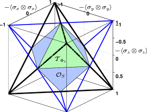
Figure 2: (Color online) State space for Bell-diagonal states. The set of physical states is the tetrahedron $\mathcal{T}_{0}$ whose edges are marked with thick (black) lines whereas the set having positive partial transpose is another tetrahedron whose edges are marked with thinner (blue) lines. The intersection of the two tetrahedra gives rise to the octahedron $\mathcal{O}_{S}$ (blue) which is the set of separable Bell-diagonal states. Entangled Bell-diagonal states satisfying Eq. (34) are contained within the tetrahedron $\mathcal{T}_{\Phi_{1}}$ (green), which is discussed further in Fig. 3.

III.3 Complete Set of SLOCC Monotones for Bell-diagonal States

Now, let us make use of the above characterization to derive a complete set of non-increasing SLOCC monotones for Bell-diagonal states. To begin with, we recall that the set of normalized Bell-diagonal states forms a tetrahedron $\mathcal{T}_{0}$ in $\mathbb{R}^{3}$, and the set of separable Bell-diagonal states forms an octahedron $\mathcal{O}_{S}$ (see Fig. 2) that is contained in $\mathcal{T}_{0}$ K.G.H.Vollbrecht:PRA:2001 . We will follow Ref. K.G.H.Vollbrecht:PRA:2001 and use the expectation values $(-\langle\sigma_{x}\otimes\sigma_{x}\rangle,-\langle\sigma_{y}\otimes\sigma_{y}\rangle,-\langle\sigma_{z}\otimes\sigma_{z}\rangle)$ as the coordinates of this three-dimensional space. The coordinates of the four Bell states $\{|\Phi_{i}\rangle\}_{i=1}^{4}$ are then $(-1,1,-1)$, $(1,-1,-1)$,$(-1,-1,1)$ and $(1,1,1)$ respectively.

Since Bell-diagonal states are convex mixtures of the four Bell projectors, we may also label any point in the state space of Bell-diagonal states by a four-component weight vector $\vec{\lambda}=(\lambda_{1},\lambda_{2},\lambda_{2},\lambda_{4})$ such that the corresponding Bell-diagonal state reads

$$\rho_{\text{BD}}(\vec{\lambda})=\sum_{i}^{4}\lambda_{i}\Pi_{i}.$$ (33)

Moreover, as remarked above, we can apply local unitary transformation to swap any of the two Bell projectors while leaving others unaffected. Thus, without loss of generality, we will restrict our attention to Bell-diagonal states such that

$$\lambda_{1}\geq\lambda_{2}\geq\lambda_{3}\geq\lambda_{4},$$ (34)

and determine when it is possible to transform between two such states under SLOCC.

Figure 3: (Color online) Tetrahedron $\mathcal{T}_{\Phi_{1}}$ (with edges marked with thick black lines) is the set of Bell-diagonal states with $\lambda_{1}\geq 1/2$. Its four vertices are the Bell state $|\Phi_{1}\rangle$ (marked with a $\bigtriangledown$) and the three separable states $\vec{\lambda}_{12}$, $\vec{\lambda}_{13}$ and $\vec{\lambda}_{14}$. Within $\mathcal{T}_{\Phi_{1}}$ is the convex polytope $\mathcal{P}_{\lambda}$, which are points within $\mathcal{T}_{\Phi_{1}}$ that can be obtained from $\vec{\lambda}$ (marked with a $\star$) by performing SLOCC transformations. Three of the facets of $\mathcal{P}_{\lambda}$, namely $\mathcal{F}_{1}$, $\mathcal{F}_{2}$ and $\mathcal{F}_{3}$ are shown with cyan, green and light purple colors, respectively; the other facets of $\mathcal{P}_{\lambda}$ are shown with blue color.

Clearly, any (entangled) Bell-diagonal state can be transformed to any separable Bell-diagonal state via SLOCC – one can simply discard the original Bell-diagonal state and prepare the separable state using LOCC. Also separable Bell-diagonal states can only be transformed among themselves with SLOCC.

What about transformations among entangled Bell-diagonal states? To answer this question, we shall adopt the following strategy. Firstly, we will clarify – in relation to Fig. 2 – the set of entangled Bell-diagonal states satisfying Eq. (34). Then, we will make use of the characterization obtained in Sec. III.2 to determine the set of states that can be obtained from SLOCC transformations when we have an input (entangled) state satisfying Eq. (34). After that, we will restrict our attention to the subset of these output states satisfying Eq. (34). Once we have got this, a simple set of necessary and sufficient conditions can be derived to determine if an entangled Bell-diagonal state can be converted to another.

We now take a closer look at the set of entangled Bell-diagonal states, in particular those that satisfy Eq. (34). In Fig. 2, the set of entangled Bell-diagonal states is the relative complement of the (blue) octahedron $\mathcal{O}_{S}$ in the tetrahedron $\mathcal{T}_{0}$. In this set, those points that satisfy Eq. (34) are a strict subset contained in the (green) tetrahedron $\mathcal{T}_{\Phi_{1}}$, which has the Bell state $|\Phi_{1}\rangle$ and the three mixed separable states

$$\rho_{1i}=\frac{1}{2}\left(|\Phi_{1}\rangle\!\langle\Phi_{1}|+|\Phi_{i}\rangle\!\langle\Phi_{i}|\right),\quad i=2,3,4,$$ (35)

as its four vertices. In terms of weight vectors, the three separable vertices read

$$\vec{\lambda}_{12}=\frac{1}{2}\left(\begin{array}[]{c}1\\ 1\\ \cdot\\ \cdot\end{array}\right),\vec{\lambda}_{13}=\frac{1}{2}\left(\begin{array}[]{c}1\\ \cdot\\ 1\\ \cdot\end{array}\right),\vec{\lambda}_{14}=\frac{1}{2}\left(\begin{array}[]{c}1\\ \cdot\\ \cdot\\ 1\end{array}\right).$$ (36)

$\mathcal{T}_{\Phi_{1}}$ is the set of Bell-diagonal states satisfying $\lambda_{1}\geq 1/2$ which includes both entangled states (denoted by $\mathcal{T}_{E}$) and separable states (denoted by $\mathcal{F}_{0}$). For the purpose of subsequent discussion, it is important to note that every entangled state satisfying Eq. (34) is in $\mathcal{T}_{E}$ but not every state in $\mathcal{T}_{E}$ satisfies Eq. (34).

Now, let us consider an entangled Bell-diagonal state $\rho_{\text{BD}}(\vec{\lambda})$ with weight vector

$$\vec{\lambda}=\left(\begin{array}[]{c}\lambda_{1}\\ \lambda_{2}\\ \lambda_{3}\\ \lambda_{4}\end{array}\right)$$ (37)

satisfying Eq. (34). Note from the above discussion that $\vec{\lambda}\in\mathcal{T}_{E}$. Recall that our goal is to determine the set of (entangled) output states – satisfying Eq. (34) – which can be obtained from $\vec{\lambda}$ via SLOCC. To achieve that, we will begin by first determining the set of output weight vectors $\{\vec{\lambda}^{\prime}\}$ which are in the superset $\mathcal{T}_{\Phi_{1}}$.

In particular, we note that under extremal SLOCC transformations associated with $G_{0}$, and the operators local unitarily equivalent to it [c.f. Eq. (6) and Sec. III.2], $\vec{\lambda}$ can be brought into any of the separable states $\{\rho_{1i}\}_{i=2}^{4}$ [c.f. Eqs. (35) and (36)]. Similarly, under extremal SLOCC transformations associated with $D_{0}$, and the operators local unitarily equivalent to it, $\vec{\lambda}$ can be brought into any of the following entangled Bell-diagonal states by permuting the weights associated with some of the Bell projectors:

$$\vec{\lambda}_{(34)}=\left(\begin{array}[]{c}\lambda_{1}\\ \lambda_{2}\\ \lambda_{4}\\ \lambda_{3}\end{array}\right),\vec{\lambda}_{(324)}=\left(\begin{array}[]{c}\lambda_{1}\\ \lambda_{3}\\ \lambda_{4}\\ \lambda_{2}\end{array}\right),\vec{\lambda}_{(24)}=\left(\begin{array}[]{c}\lambda_{1}\\ \lambda_{4}\\ \lambda_{3}\\ \lambda_{2}\end{array}\right),$$ (50)

$$\vec{\lambda}_{(234)}=\left(\begin{array}[]{c}\lambda_{1}\\ \lambda_{4}\\ \lambda_{2}\\ \lambda_{3}\end{array}\right),\vec{\lambda}_{(23)}=\left(\begin{array}[]{c}\lambda_{1}\\ \lambda_{3}\\ \lambda_{2}\\ \lambda_{4}\end{array}\right).$$ (59)

Evidently, any convex combinations of the vectors listed in Eq. (36), Eq. (37) and Eq. (59) are also attainable from $\vec{\lambda}$ using (non-extremal) SLOCC. Moreover, within $\mathcal{T}_{\Phi_{1}}$, only convex combinations of these states, denoted by $\mathcal{P}_{\lambda}$, are attainable from $\vec{\lambda}$ using SLOCC. $\mathcal{P}_{\lambda}$ is thus a convex polytope with vertices given by the union of vectors listed in Eq. (36), Eq. (37) and Eq. (59).

Then, to determine if $\vec{\lambda}$ can be transformed to another $\vec{\lambda^{\prime}}\in\mathcal{T}_{\Phi_{1}}$ amounts to deciding if $\vec{\lambda^{\prime}}\in\mathcal{P}_{\lambda}$. It is a well known fact that a convex polytope can also be described by a finite set of inequalities that are associated with each of the facets of the polytope B.Grunbaum:polytope . Therefore, the above task can be done, for example, by checking if $\vec{\lambda^{\prime}}$ satisfies all the linear equalities defining the polytope $\mathcal{P}_{\lambda}$.

Our real interest, however, is in the set of entangled Bell-diagonal states satisfying Eq. (34). With some thought, it should be clear that this simplifies the problem at hand so that we will only need to check that $\vec{\lambda^{\prime}}$ satisfies all the inequalities (facets) that contain $\vec{\lambda}$. From Fig. 3, it can be seen that only three facets of $\mathcal{P}_{\lambda}$ contain $\vec{\lambda}$. These are $\mathcal{F}_{1}=\text{conv}\{\vec{\lambda},\vec{\lambda}_{(34)},\vec{\lambda}_{(324)},\vec{\lambda}_{(24)},\vec{\lambda}_{(234)},\vec{\lambda}_{(23)}\}$, $\mathcal{F}_{2}=\text{conv}\{\vec{\lambda},\vec{\lambda}_{12},\vec{\lambda}_{(34)}\}$ and $\mathcal{F}_{3}=\text{conv}\{\vec{\lambda},\vec{\lambda}_{12},\vec{\lambda}_{13},\vec{\lambda}_{(23)}\}$, where $\text{conv}\{.\}$ represents the convex hull formed by the set of points in $\{.\}$ B.Grunbaum:polytope .

Recall that each vector $\vec{\lambda}_{(.)}$ listed in Eq. (59) is obtained by performing the appropriate permutation $(.)$ on all but the first component of $\vec{\lambda}$. Hence $\mathcal{F}_{1}$ is a facet of constant $\lambda_{1}$. After some simple algebra, the inequalities associated with $\mathcal{F}_{2}$ fn:F2 and $\mathcal{F}_{3}$ fn:F3 can be shown to be, respectively,

$$\mathcal{F}_{2}:\frac{\lambda_{3}+\lambda_{4}}{\lambda_{1}-\lambda_{2}}\left(\langle\sigma_{x}\otimes\sigma_{x}\rangle-\langle\sigma_{y}\otimes\sigma_{y}\rangle\right)+\langle\sigma_{z}\otimes\sigma_{z}\rangle\leq 1,$$ (60)

$$\mathcal{F}_{3}:\langle\sigma_{x}\otimes\sigma_{x}\rangle+\langle\sigma_{z}\otimes\sigma_{z}\rangle-\frac{1-2\lambda_{1}+2\lambda_{4}}{1-2\lambda_{2}-2\lambda_{3}}\langle\sigma_{y}\otimes\sigma_{y}\rangle\leq 1.$$ (61)

Imposing the requirement that $\vec{\lambda^{\prime}}$ satisfies these inequalities gives, respectively,

$$\frac{1-2\lambda_{2}}{\lambda_{3}+\lambda_{4}}\geq\frac{1-2\lambda^{\prime}_{2}}{\lambda^{\prime}_{3}+\lambda^{\prime}_{4}},$$

and

$$\frac{1-2\lambda_{2}-2\lambda_{3}}{\lambda_{4}}\geq\frac{1-2\lambda^{\prime}_{2}-2\lambda^{\prime}_{3}}{\lambda^{\prime}_{4}}.$$

Together with the requirement imposed by $\mathcal{F}_{1}$, we see that by defining

$$E_{1}(\vec{\lambda}) \equiv\lambda_{1},$$ (62)

$$E_{2}(\vec{\lambda}) \equiv\frac{1-2\lambda_{2}}{\lambda_{3}+\lambda_{4}},$$ (63)

$$E_{3}(\vec{\lambda}) \equiv\frac{1-2\lambda_{2}-2\lambda_{3}}{\lambda_{4}},$$ (64)

the intercovertibility between two entangled Bell-diagonal states can be succinctly summarized in the following theorem.

Theorem 4.

Let $\rho$ and $\rho^{\prime}$ be two entangled Bell-diagonal states with, respectively, weight vectors $\vec{\lambda}$ and $\vec{\lambda}^{\prime}$ satisfying Eq. (34). Transformation from $\rho$ to $\rho^{\prime}$ via SLOCC is possible iff

$$E_{1}(\vec{\lambda})\geq E_{1}(\vec{\lambda^{\prime}}),$$ (65)

$$E_{2}(\vec{\lambda})\geq E_{2}(\vec{\lambda^{\prime}}),$$ (66)

$$E_{3}(\vec{\lambda})\geq E_{3}(\vec{\lambda^{\prime}}).$$ (67)

In other words, $\{E_{i}(\vec{\lambda})\}_{i=1}^{3}$ is a complete set of SLOCC monotones for entangled Bell-diagonal states satisfying Eq. (34).

IV SLOCC Convertibility of Two-Qubit States

With Theorem 4, it is just another small step to determine if a two-qubit state $\rho$ can be converted to another, say $\rho^{\prime}$ using SLOCC. To this end, let us first recall the following definition from Ref. W.Dur:PRA:2000 .

Definition 5.

Two states $\rho$ and $\rho^{\prime}$ are said to be SLOCC equivalent if $\rho$ can be converted to $\rho^{\prime}$ via SLOCC with nonzero probability and vice versa.

Next, we recall the following theorem, which can be deduced from Theorem 1 in Ref. F.Verstraete:PRA:2002 (see also Theorems 1–3 in Ref. F.Verstraete:PRA:2001 ).

Theorem 6.

A two-qubit state $\rho$ is SLOCC equivalent to either (1) a unique Bell-diagonal state satisfying Eq. (34), (2) a separable state, or (3) a (normalized) non-Bell-diagonal state of the form:

$$\rho_{\rm ND}=\frac{1}{4}\left(\begin{array}[]{cccc}2&\cdot&\cdot&\cdot\\ \cdot&1&2b&\cdot\\ \cdot&2b&1&\cdot\\ \cdot&\cdot&\cdot&\cdot\end{array}\right),$$ (68)

where $\rho_{\rm ND}$ is expressed in the standard product basis and $b\leq\frac{1}{2}$ is unique.

Moreover, as was shown in Ref. F.Verstraete:PRA:2001 , the unique Bell-diagonal state in case (1) is the state with maximal entanglement that can be obtained from the original two-qubit state using SLOCC. The two-qubit state associated with case (2) is clearly a separable one since a separable state is, and can only be, SLOCC equivalent to another separable state.

The situation for case (3) is somewhat more complicated and the original two-qubit states associated with this case are either of rank 3 or 2 (in the case of $b=1/2$)  LX.Cen ; F.Verstraete:PRA:2001 ; F.Verstraete:PRA:2002 . By very inefficient SLOCC transformations – quasi-distillation MPR.Horodecki:PRA:1999 – the entanglement in the equivalent state $\rho_{\text{ND}}$ can be maximized by converting it into the following Bell-diagonal state:

$$\rho_{\rm ND}^{\prime}=\frac{1}{2}\left(\begin{array}[]{cccc}\cdot&\cdot&\cdot&\cdot\\ \cdot&1&-2b&\cdot\\ \cdot&-2b&1&\cdot\\ \cdot&\cdot&\cdot&\cdot\end{array}\right).$$ (69)

However, it remains unclear from existing results LX.Cen ; MPR.Horodecki:PRA:1999 ; F.Verstraete:PRA:2001 ; F.Verstraete:PRA:2002 if this process is reversible fn:reverse . In this regard, we have found that the reverse process can indeed be carried out via a separable map with two terms involved in the Kraus decomposition. In particular, a possible form of the Kraus operators associated with this separable map reads [Eq. (26)]:

$$A_{1}=\left(\begin{array}[]{cc}-2b+\sqrt{1+4b^{2}}&-1/2\\ 1&\cdot\end{array}\right),\quad B_{1}=\left(\begin{array}[]{cc}1&1/2\\ 1&\cdot\end{array}\right),$$

$$A_{2}=\left(\begin{array}[]{cc}2b-\sqrt{1+4b^{2}}&1/2\\ 1&\cdot\end{array}\right),\quad B_{2}=\left(\begin{array}[]{cc}1&1/2\\ -1&\cdot\end{array}\right).$$

Thus, a two-qubit state that is SLOCC equivalent to $\rho_{\text{ND}}$ is also SLOCC equivalent to a unique Bell-diagonal state $\rho_{\text{ND}}^{\prime}$. By further local unitary transformation, we can bring $\rho_{\text{ND}}^{\prime}$ into a form that satisfies Eq. (34). Hence, this leads us to the following theorem.

Theorem 7.

All entangled two-qubit states are SLOCC equivalent to a unique Bell-diagonal state satisfying Eq. (34).

With this theorem, one can now readily determine if an entangled two-qubit state $\rho$ can be converted to another, say, $\rho^{\prime}$, using SLOCC. For that matter, let $\rho_{\text{BD}}(\vec{\lambda})$ and $\rho_{\text{BD}}(\vec{\lambda}^{\prime})$ be, respectively, the unique Bell-diagonal state satisfying Eq. (34) that is SLOCC equivalent to $\rho$ and $\rho^{\prime}$. Then, it follows from Theorem 4 that $\rho$ can be transformed to $\rho^{\prime}$ using SLOCC if and only if the corresponding weight vectors of the associated Bell-diagonal states $\vec{\lambda}$ and $\vec{\lambda}^{\prime}$ satisfy Eqs. (65)-(67). In other words, the SLOCC convertibility of two two-qubit states can be decided via the following theorem.

Theorem 8.

Let $\rho_{\text{BD}}(\vec{\lambda})$ and $\rho_{\text{BD}}(\vec{\lambda}^{\prime})$ be, respectively, the Bell-diagonal state satisfying Eq. (34) that is SLOCC equivalent to $\rho$ and $\rho^{\prime}$. $\rho$ can be locally transformed onto $\rho^{\prime}$ with nonzero probability if and only if (1) $\rho^{\prime}$ is separable or (2) $\rho$ is entangled and the associated weight vectors $\vec{\lambda}$ and $\vec{\lambda}^{\prime}$ satisfy Eqs. (65)-(67).

Schematically, if neither $\rho$ nor $\rho^{\prime}$ are separable and if Eqs. (65)-(67) are satisfied, then one possible way of transforming $\rho$ to $\rho^{\prime}$ via SLOCC is by performing the following chain of conversions:

$$\rho\to\rho_{\text{BD}}(\vec{\lambda})\to\rho_{\text{BD}}(\vec{\lambda}^{\prime})\to\rho^{\prime},$$

whereas if any one of Eqs. (65)-(67) is not satisfied, then

$$\rho\not\to\rho^{\prime}.$$

V Discussion and Conclusion

In this paper, we have investigated the bi-separability of the set of four-qubit states commuting with $U\otimes{U}\otimes{V}\otimes{V}$ where $U$ and $V$ are arbitrary members of the Pauli group. These are essentially convex combination of two (not necessarily identical) copies of Bell states. Evidently, these states are all separable across the two copies. For the other bi-partitioning, we have found that the separable subset is a convex polytope and hence can be described by a finite set of entanglement witnesses.

Equivalently, this characterization has also given us the complete set of separable, Bell-diagonal preserving, completely positive maps. This has enabled us to derive a complete set of SLOCC monotones for Bell-diagonal states, which can be used to determine if a Bell-diagonal state can be converted to another using SLOCC.

We have then supplemented the result on SLOCC equivalence presented in Refs. F.Verstraete:PRA:2001 ; F.Verstraete:PRA:2002 to arrive at the conclusion that all entangled two-qubit states are SLOCC equivalent to a unique Bell-diagonal state. Combining this with the SLOCC monotones that we have derived immediately leads us to some simple necessary and sufficient criteria on the SLOCC convertibility between two-qubit states.

- (1) L. Gurvits, in Proceedings of the Thirty-Fifth ACM Symposium on Theory of Computing (ACM, New York, 2003), pp. 10-19; L. M. Ioannou, Quant Inf. Comput. 7, 335 (2007).
- (2) A. Peres, Phys. Rev. Lett. 77, 1413 (1996); M. Horodecki, P. Horodecki, R. Horodecki, Phys. Lett. A 223, 1 (1996).
- (3) R. F. Werner, Phys. Rev. A40, 4277 (1989).
- (4) M. Horodecki and P. Horodecki, Phys. Rev. A59, 4206 (1999).
- (5) K. G. H.Vollbrecht and R. F. Werner, Phys. Rev. A64, 062307 (2001).
- (6) T. Eggeling and R. F. Werner, Phys. Rev. A63, 042111 (2001).
- (7) M. A. Nielsen, Phys. Rev. Lett. 83, 436 (1999).
- (8) G. Vidal, J. Mod. Opt. 47, 355 (2000).
- (9) W. Dür, G. Vidal, and J. I. Cirac, Phys. Rev. A62, 062314 (2000).
- (10) G. Vidal, Phys. Rev. Lett. 83, 1046 (1999).
- (11) C. H. Bennett, H. J. Bernstein, S. Popescu, and B. Schumacher, 53, 2046 (1996).
- (12) A. Kent, N. Linden, and S. Massar, Phys. Rev. Lett. 83, 2656 (1999).
- (13) L.-X. Cen, F. -L. Li, and S. -Y. Zhu, Phys. Lett. A 275, 368 (2000); L.-X. Cen, N.-J. Wu, F.-H. Yang, and J.-H. An, Phys. Rev. A65 052318 (2002).
- (14) S. Hill and W. K. Wootters, Phys. Rev. Lett. 78, 5022 (1997).
- (15) F. Verstraete, J. Dehaene, and B. DeMoor, Phys. Rev. A64, 010101(R) (2001).
- (16) Obviously, unique up to local unitary transformations.
- (17) Maximal, in the sense that no SLOCC transformations can bring the state to another one with higher entanglement of formation.
- (18) F. Verstraete, J. Dehaene, and B. DeMoor, Phys. Rev. A65, 032308 (2002).
- (19) Ll. Masanes, Y.-C. Liang, and A. C. Doherty, e-print quant-ph/0703268.
- (20) S. Popescu, Phys. Rev. Lett. 74, 2619 (1995); N. Gisin, Phys. Lett. A 210, 151 (1996).
- (21) J. F. Clauser, M. A. Horne, A. Shimony and R. Holt, Phys. Rev. Lett. 23, 880 (1969); J. S. Bell, in Foundation of Quantum Mechanics. Proceedings of the International School of Physics ’Enrico Fermi’, course IL (Academic, New York, 1971), pp. 171-181.
- (22) Their separability can be veirfied, for example, by writing these operators in full in the product basis via Eq. (4) and showing that they admit convex decomposition in terms of separable states. Alternatively, via the Choi-Jamiołkowski isomorphism that will be discussed later in Sec. III.1 and the remarks made towards the end of Sec. III.2, one can also see that these matrices correspond to separable states.
- (23) B. Grünbaum, Convex Polytopes (Springer, New York, 2003).
- (24) This software package, which stands for POlyhedron Representation Transformation Algorithm, is available at http://www.zib.de/Optimization/Software/Porta/
- (25) A. C. Doherty, P. A. Parrilo, and F. M. Spedalieri, Phys. Rev. Lett. 88, 187904 (2002); A. C. Doherty, P. A. Parrilo, and F. M. Spedalieri, Phys. Rev. A69, 022308 (2004).
- (26) L. Vandenberghe and S. Boyd, SIAM Review 38, 49 (1996); S. Boyd and L. Vandenberghe, Convex Optimization (Cambridge, New York, 2004).
- (27) http://www.physics.uq.edu.au/qisci/yerng/
- (28) Note that to verify against Eq. (25), one should also rewrite obtained in Eq. (24) in the appropriate tensor-product basis such that acts on .
- (29) A. Jamiołkowski, Rep. Math. Phys. 3, 275 (1972); M. D. Choi, Lin. Alg. Appl. 10, 285 (1975); V. P. Belavin and P. Staszewski, Rep. Math. Phys. 24, 49 (1986).
- (30) E. M. Rains, e-print quant-ph/9707002.
- (31) V. Vedral and M. B. Plenio, Phys. Rev. A57, 1619 (1998).
- (32) Following Kraus’ work on CPM Kraus , this specific form of the CPM is also known as a Kraus decomposition of the CPM, with each in the sum conventionally called the Kraus operator associated with the CPM.
- (33) K. Kraus, State, Effects, and Operations (Springer, Berlin, 1983); Ann. Phys. (N.Y.) 64, 311 (1971).
- (34) C. H. Bennett, D. P. DiVincenzo, C. A. Fuchs, T. Mor, E. Rains, P. W. Shor, J. A. Smolin, and W. K. Wootters, Phys. Rev. A59, 1070 (1999).
- (35) J. I. Cirac, W. Dür, B. Kraus, and M. Lewenstein, Phys. Rev. Lett. 86, 544 (2001).
- (36) The derived from in Eq. (6) is an example of this sort. In fact, in this case, if the input state has no support on nor , the map always outputs the zero matrix.
- (37) Since the mapping from any to a separable CPM via Eq. (29) is only defined up to a positive constant, for the subsequent discussion, we might as well consider the cone generated by .
- (38) M. Horodecki, P. Horodecki, and R. Horodecki, Phys. Rev. A60, 1888 (1999).
- (39) Strictly, the inequality (60) is only valid when . When , degenerates into an edge of the polytope . If , collapses into a single point .
- (40) Within , only when and . In this case, degenerates into the line joining and .
- (41) By this, of course, we are referring only to the states given in Eq. (68) that are originally of rank three, and which becomes rank two upon quasi-distillation. The states given in Eq. (68) that are of rank two get quasi-distilled to the singlet state and so the process is clearly reversible in this case.