Urban and Scientific Segregation: The Schelling-Ising Model

Dietrich Stauffer and Christian Schulze
Institute for Theoretical Physics, Cologne University
D-50923 Köln, Euroland

Abstract: Urban segregation of different communities, like blacks and whites in the USA, has been simulated by Ising-like models since Schelling 1971. This research was accompanied by a scientific segregation, with sociologists and physicists ignoring each other until 2000. We review recent progress and also present some new two-temperature multi-cultural simulations.

1 Introduction

The Schelling-Ising model of urban segregation is for two reasons of interest for readers of sociophysics [1] papers: 1) It may explain aspects of racial, ethnic, religious, … segregation in large cities (“ghetto formation”); 2) it is an example of decades-long non-cooperation between social sciences and physics.

Harlem in New York City, USA, is the “black” residential district of Manhattan, where hundreds of thousands of Afro-Americans live. In most of the rest of Manhattan the population is at least 80 percent “white” (ignoring Hispanic), while Harlem is at least 80 percent ”black” [2]. Similar residential segregation has been observed in other places, along ethnic, religious or other barriers, though often on a smaller scale. The city of the present authors [3] has since years a tenth of its population from Turkish background and now it tries to deal with a plan to build a large mosque here, after years of partial segregation into several “Turkish” city districts.

Such segregated residential districts can be caused by external forces, like the orders of Nazi Germany that all Jews have to live in small ghettos of Warsaw, Cracow, …. The alternative to be discussed here is the emergence of urban segregation without external force, only through self-organisation due to the wishes of the residents.

This second possibility was already pointed out 25 centuries ago by the Greek philosopher Empedokles, who (according to J. Mimkes) found that humans are like liquids: some live together like wine and water, and some like oil and water refuse to mix. This idea was formulated more clearly by the German poet Johann Wolfgang von Goethe in “Wahlverwandtschaften” two centuries ago (also according to J. Mimkes). The rest of this article deals with the implementation of this basic idea.

Schelling published in 1971 the first quantitative model for the emergence of urban segregation [4], in the same year in which physicist Weidlich [5] published his first paper on sociodynamics. Schelling in 2005 got the economics “Nobel” prize; his 1971 paper has an exponentially rising citation rate and is the second-most-cited paper in this Journal of Mathematical Sociology. His model is a complicated zero-temperature Ising ferromagnet but this similarity to statistical physics was overlooked [6]. Only very recent publications [7, 8] pointed out that Schelling’s original model fails to form large ghettos and leads only to small clusters of residences for the two groups in the population. Long before, Jones [9] introduced some randomness into the model to produce large ghettos; this good paper, in turn, was mostly ignored for two decades.

The first citation to Schelling 1971 from physicists known to us is the book of Levy, Levy and Solomon [10], nearly three decades after publication. One of us (DS) learned about the Schelling model from a meeting on Simulating Society in Poland, fall 2001 (though he should have learned it from [10] of which he got preprints). He then was advised in spring 2002 by Weidlich [5] to study learning for urban segregation, and forwarded this idea to [11, 12]. Vinkovic and Kirman [7] reviewed nicely the physics of hundred years ago in the Empedokles-Goethe sense, but ignored the physics research of recent decades. We are not aware of sociology to have taken note of the Ising model in the follow-up of the Schelling model [4]; as mentioned sociologists also mostly ignored the paper of their colleague Jones [9] in a sociology journal.

Thus we see here not only residential segregation, but also scholarly segregation, with physicists ignoring the Schelling model until recently, and sociologists ignoring the similarity of the Schelling to the Ising model until now. Books like the present one can help to bridge the gap.

This article is written for physicists; an earlier article [8] was supposed to help also non-physicists understand the Ising model in connection with urban segregation.

2 Schelling model

In order to check whether urban segregation can emerge from personal preferences without any overall management, discrimination etc, Schelling published in 1971 a modification of the spin 1/2 Ising model at zero temperature. The majority of sites on a square lattice are occupied by people who belong to one of two groups A and B. The initial distribution is random: A and B in equal proportion; a minority of sites is empty. Everybody likes to be surrounded by nearest and next-nearest neighbours of the same kind. People are defined as unhappy if the majority of their neighbours belongs to the other group, and as happy if at least half of these neighbours belong to the own group. (Empty sites do not count in this determination.) At each iteration with random sequential updating, unhappy people move to the nearest place where they can be happy [4].

As a result, clusters are formed where A residences stick together, and also B people cluster together. These clusters remain also when details of the model, like the thresholds of happiness, are changed [4]. The lattices studied (by hand !) in that paper were too small to indicate whether the clusters become infinite in an infinite lattice, i.e. whether phase separation like oil in water happens. Only a third of a century later, a computational astrophysicists and an economist [7] showed that the clusters remain small even if large lattices are simulated. Thus the original Schelling model is unable to explain the formation of large ghettos like Harlem, but it can explain the clustering of a few B residences surrounded by A houses. We have not yet found papers from sociology pointing out this failure, though Jones [9] may have noticed it when he improved the model (see below), without stating it explicitly in his publication.

Even without any computer simulation one can guess that the original Schelling model had troubles. Solomon [8] pointed out that the following B cluster will never dissolve from within: Each B has four or more B sites in its neighbourhood of eight, feels happy and has no intention to move. The A have even less reason to move.

A A A A A A A A

A A A A A A A A

A A A B B A A A

A A B B B B A A

A A B B B B A A

A A A B B A A A

A A A A A A A A

A A A A A A A A

Also horizontal strips of A and B sites lead to blocking, as in Ising models [13], since even at the interface everybody is happily surrounded by neighbours mostly of the own group. To avoid such blocking of cluster growth, Jones [9] removed a small fraction of people randomly, and replaced them by people who feel happy in these vacancies. Then really large ghettos are formed. (The earlier Dethlefsen-Moody model also involves randomness and still gives only finite clusters, though larger than in the Schelling version, according to Müller [14].)

An alternative way to introduce some randomness [7] is to allow people to move even when their status (happy or unhappy) is not changed by this move. Then domains were simulated to grow towards infinity, and the detailed behaviour of this growth process was studied later [15]. This assumption seems at first sociologically nonsensical: Why should anyone go through the troubles to move if this does not improve the situation?

However, one may regard such “useless” moves as coming from forces external to the model, like when one moves to another city in order to switch employment. In that case, however, one may also be forced from a happy place to one where one feels unhappy, as is done below through a finite temperature $T$. Thus the model of [7, 15] is a nice physics model with limited sociological appeal.

[Schelling assumed that A people stay A people forever, and the same applies to B people. This may not be true with respect to religion or citizenship but is correct with respect to skin colour. However, people also move out into another city, or in from another city, and thus within the simulated area the number of A and B people can change. The blacks in Harlem may have had ancestors who worked on tobacco or cotton plantations, but these plantations were further south and not in Manhattan. Jones [9] already simulated fluctuating compositions, and in contrast to an assertion in [7], the Ising models has been simulated since decades for both fixed (Kawasaki) and fluctuating (Glauber, Metropolis) magnetisations.]

3 Two groups, one temperature

3.1 Schelling and Ising at positive $T$

Life is unfair, and we do not always get what we want. Thus for accidents outside the model, like loss of job, marriage, …, we sometimes have to change residences even if we like the one in which we live. Thus we may not only have neutral moves as in [7] from unhappy to unhappy or from happy to happy, but also from happy to unhappy with some low probability. This is the basis of thermal Monte Carlo methods (Metropolis, Glauber, Heat Bath algorithm), also for optimization (simulated annealing etc.) [16], where the energy (unhappiness) is increased by $\Delta E$ with a probability $\propto\exp(-\Delta E/k_{B}T)$. And then it also makes sense to look at different degrees of (un)happiness, that means to treat the number of neighbours from the other group as $\Delta E$. The standard two-dimensional Ising model then is the simplest choice.

In this sense, $T$ plays the strength of the external noise which pushes us to move against our personal preferences. Instead, the temperature $T$ can also be interpreted as “tolerance” [17]: The higher $T$ is, the more are we willing to live with neighbours of the other group. In the limit of infinite $T$ the composition of the neighbourhood plays no role for changing residences; in the opposite limit of zero $T$ we never move from happy to unhappy in the Schelling version; and never from a smaller to a larger number of “wrong” neighbors in the Ising version. In the Ising version, again one can work with a constant or a fluctuating composition of the total population.

In the Schelling version at finite $T$, with probability exp($-1/T$) we consider moving out of a site where we are happy, and we always consider moving out from a site where we are unhappy [8]. If we consider moving, we check empty sites in order of their distance from us, and accept the new site if we are happy there. Otherwise we accept it only with probability exp($-1/T$) if we are unhappy there, and instead continue to look for empty sites further away with probability $1-\exp(-1/T)$. Then large ghettos are formed though very slowly [8]. Similar results are found in various variants [14].

In the Ising version at finite $T$ we have much simpler and clearer definitions and flip a spin (change the group at one site) with probability $1/[1+\exp(\Delta E/k_{B}T)]$. The degree $\Delta E/J$ of unhappiness is the number of neighbours of the other group, minus the number of neighbours of the same group. Thus, for example, neutral moves [7] are made with probability 1/2, and moves from four neighbors of the own group to four neighbours of the other group only with probability exp$(-8J/k_{B}T)$ at low $T$. (The proportionality constant $J$ is called exchange energy in physics.) This Ising model shows growth of infinitely large domains (“ghettos”) for $T<T_{c}$ and only finite clusters for $T>T_{c}$ with $J/k_{B}T_{c}=\ln(1+\sqrt{2})/2$, as is known since two-thirds of a century. Such pictures are also nice for teaching [18].

More novel Ising simulations [11] took into account the “learning”: Through education etc people become more tolerant of others or more similar to others. Thus Meyer-Ortmanns [11] showed how at low tolerance $T$ compact ghettos are formed, which dissolve through Kawasaki kinetics (constant composition of the population) if $T$ is suddenly increased. It does not matter whether this learning comes from the groups becoming more similar to each other (decrease of $J$) or from both groups increasing their tolerance $T$: Only the ratio $J/k_{B}T$ enters the simulations. We will return to this learning when dealing with more than two groups in a Potts-like segregation model [12].

V.Jentsch and W.Alt at Bonn University’s complexity centre suggested to have an individual $T(i)$ for each different site $i$, and to introduce a feedback: If one sees that all neighbours are of the own group, one realizes that strong segregation has happened, does not like this effect, and thus increases the own $T(i)$ by 0.01. If, in contrast, all neighbours belong to the other group, one also dislikes that and decreases the own $T(i)$ by 0.01. Also, one forgets the tolerance one has learned this way and decreases $T(i)$ at each time step by a fraction of a percent. Then [14] depending on this forgetting rate, a spontaneous magnetisation remains, or it goes down to zero, while the final self-organized average $T$ may differ only slightly in these two cases.

3.2 Money and random-field Ising model

Figure 1: Large domains (upper part) and small clusters (lower part) for small (0.2) and large (1.5) random fields, respectively, at $T=1$. Field and temperature are measured in units of $J/k_{B}$. After [20].

Often, a population can be approximately divided into rich and poor. Starving associate professors and luxuriously living full professors are one example, but poorer immigrants and richer natives are more widespread. Poor people cannot afford to live in expensive houses, but rich people can. If there are whole neighbourhoods of expensive and cheap housing, then these housing conditions enforce a segregation of rich from poor, and this segregation does not emerge in a self-organised way. The more interesting case allows for self-organisation of domains by assuming that each residence randomly is either expensive or cheap, with no spatial correlations in the prices. Does this model lead to spatial correlations between the two groups, assumed as poor and rich?

A suitable model is the random-field Ising magnet, where each site of a square lattice carries a magnetic field $\pm h$ which is randomly up (expensive) or down (cheap). The resulting addition to the energy prefers up spins on the expensive and down spins on the cheap sites. Simulations of the asymptotic behaviour are difficult [19], but are not needed for urban segregation happening in finite times on finite samples [20]. Fig.1 shows two examples: A small random field allows for large domains, upper part, while a large random field allows only small clusters, lower part. Sumour et al [20] presented at lower temperatures also a time series of pictures, separating growing from non-growing domains. They also listed a complete 50-line Fortran program.

Thus we see that the personal preferences are balanced by the random field, i.e. by the prices of housing; spatial correlations over short distances still exist for moderately high fields.

4 Several groups, two temperatures

While the separation into black and white corresponds to USA traditions, reality often means the coexistence of more than two major groups (like Hispanics in the USA). Similarly, while the spin 1/2 Ising model is the most basic and most widespread model in statistical physics, the Potts and Blume-Capel models have generalized it to more than two possible states of each lattice site [12].

Also, while equilibrium physics has one temperature $T$, in the above segregation studies we used $T$ for both the tolerance [17] and the external noise [8]. In reality, these two effects should be described by two independent parameters $T_{1}$ for tolerance and $T_{2}$ for noise. And again the tolerance can be different for different people and can self-organize to some average tolerance through a feedback with the local amount of segregation, as discussed above for two states and one local temperature.

If each site $i$ of a lattice carries a variable $q_{i}=1,2,\dots,Q$, it may correspond to $Q$ different ethnic groups. For Germany, $Q=5$ may represent immigrants from the Iberian peninsula ($q=1$), from Italy ($q=2$), from the former Yugoslavia ($q=4$), from Turkey ($q=5$) and native German tribes ($q=3$). The more dissimilar these groups are, the less they like each other. Thus the energy $E$ or unhappiness is assumed to be

$$E=J\sum|q_{i}-q_{k}|$$

where the sum goes over all nearest neighbour pairs on a $L\times L$ square lattice, with helical boundary conditions. We measure all temperatures in units of the Potts critical temperature [2/ln$(1+\sqrt{Q})]J/k_{B}$, even though this model does not have a sharp phase transition for $Q>2$ [12]; only for $Q=2$ is $T=1$ at the Curie temperature or segregation point. People exchange residences with others anywhere in the system (except in their immediate neighbourhood), with Glauber probability $1/[1+\exp(\Delta E/k_{B}T)]$, thus the number of members of the $Q$ groups remains the same.

As in the above Ising case [11], we allow for learning. Here that means we start at a low temperature 0.5 and with increasing time $t$ we increase $T$ during a learning time $\tau$ to a higher temperature 2.5 according to

$$T(t)=0.5+2t/\tau$$

We measure the amount of segregation through the correlation

$$C(t)=\langle n\rangle Q/4$$

where $n$ is the number of nearest neighbours of the same group and averaged over all sites. (Alternatively one can average only over the sites occupied by the central group.) In this way, $C=1$ for the initial random distribution of people, and the increase of $C$ above unity measures the amount of segregation.

The following picture shows a small configuration at $\tau=0$, i.e. when the tolerance is immediately at its maximum final value $T=2.5$; hundred sweeps through the lattice were made, and only the central group 3 for $Q=5$ is shown.

                *  ** * *            **         *                    *  * *   **
       *           * **                      *                          *** *
           *     ** ****      *        *    **        *   *          *   **  *
 * *                  ** *          *  * **** ***                   **   *    *
   *    *  *                  *      ***********          *        **       *
          ***        *              ***   * ****                   ** **
  *  *    *  * **                         **  ***      *            ****
       *  **  ****               ***           *      **        ** *  *   *   **
           * *            *       **  *        *      **       * * *****  ****
   * *  ****  *           **      *   * **     *    ***  *        * * *
    ***** ***                                  *     *   *    *    ** ***
    *  *   **   *  **                    **          * ****   **      **   *
     *                       *     *             ** ***  * **        *  *
 *      *    **                                ****  ***                *
   *   *  **   * **          * *                **    **     *                **
 *  **     * *     *          ***     *        *    *         *          *    **
 *   *  *                        **  **     *     *    *   **  * **         **
                  *     *     ** *   *   **   * *            *** **        * **
     *                      * **     *    *                    **            *
                  **       *  ***       *    *              **      *
 *  **               *        **         *  **              *
    * *          **           *     ****                   **     *
      *****      *   ***       **   ****                          *            *
      *** *                   ***               *        *
      **   ** *****      **     **    *       * *       *  *              *
            *  *        **             *      *          **
   ***              *  ****                             **          * **
    **                 * **      *     *       *        ***           **
    ** *          *   **     *  *   * **                 **      *
    *   ***   ** **       *   **    *         *         *   **                 *
      ****     **               **  **                      * *  **
        **      * *               *                  *        *  *       *
  * *   *              * *                     *      **       *        **  *  *
   *          *   *    * ***   ** *        **  **    *                ******  *
                        * *      **                 *               * * *** **
                **     **     **              ** ** *                **   **
       **   **  *     **       ***  *    *       ** *                 **      *
      ***   * **   *    *       *  **           *        *               ** *
     **** ****  ****               *          ***                       ***   *
     ** ** *  * ****          *   **       *    **                       * *  *
    ** * **   * *  ***     *          *       ** *                            *
      * *        *  *     *       **      *****
         * *         *    *         *  *    ** *        *                 *
            * *               *     * *    **                              *
            *                      *       *** **
             *  *          *** *  **     *  ***                       *
  *            **         ****     **          *        *         **  **
            *            *  * **  *       * ****                 *    **
                      * *    *  * *   ******** ***                     *
                      *****     *   **  *    *   **                  ***
   *                *           *   **  * *      ***  **              **
                    *  *   *       **           **  *  *     *         *
    *               *   *    *           *      * *   **** * **         *      *
   *             *   *       *                    *  **   ** **   *     *   * *
      *  *       **  ** **      *                **  *    ***    **  *
      *    *        **  *                               ** ***    ****  *
       *  **      *     ****  **** **                *     *    **   *
      *    *              *    *    *               *                *
  *   *       *                *    *                *           *       *
  **  * **             **   ****   **                            * *    **     *
    *                   *** *      *     *  *                    ****   *
                     ***  ***  *           ***      *   *  *     *  **
   ***               ****             **  ****     ***  *        **  *         *
    **               ***  *            ******     *****        *        * *  *
            *                          * **         * **  * *  *          ****
                **     *    *   *      *    *       **         *     * ****  * *
 *          * *    *        *        * *****                ****      ***** *
 *        * ***          *     *  *    * ***    * ****       *   *       ***  *
 * **  **  ***   *      *  *  ****  *  * **** **             *      *  ** *   **
  **  *** ** ****  *** ***   **     *  *    ****  **                    **
     *****   *** **  ** **          ****  *      ****       **           * *
   ****     ***      *           * **       **   **               *          *
    ** **   *     ** **  *              *         **   *         *           **
            *   *   ****                **    **  ***                ***      *
            ** *    ***  *              *** *  ** * *                * *      *
  *      *  *  ****                         * *  ** * ***
 ***        **  * *    **            *           *      ******
   *    *     *       * * *       **            *      ***
  ***      * ** *  ***  *          * *    *            *                    *  *

Now we bring the corresponding configuration for much slower learning $\tau=20$:

 *  ****       **  ***       ** *** ***   *****     ***             ** * *
  ******       *** *            *******    **       *     *
   ******      *****     *  **   ******     *       *
    ****     ********         ********              *
           *   **               *   *


                                                  *
         *                                   **  *                    **   ***
        **                                   *** *                 **        *
       ****                                *******                 **
       ******                             ****              *   *  **
        ******                            **                *           *
  *      **                              **                 *
  *       *******                 *****                     *         **
            *  ***              *   **                                 *
  *                                 ** * **                 *         **
  *                                 *   *                   *        *
  *                                     ***                 *        *
  *   *        *                                          ***
   ****  *** *** ***                                     **        *
   **    *** *** ******        **               ** *      *
          ***** *******       **                   *       *     **
          *************   ***                      *     ****
        **   ********** ***                        *     *****             *
        *     ***    ** **                               ** **        *
               *        ***                              *****
                         **          *                    ***                *
                          *         **         *          ***                **
                          **       *                     * ***                *
        **                **                          ********                *
        **                *                         ***********               *
       *         *        *                       ***********         ****   ***
             ******      **                         *******             **  ****
 *****         ****      **     *                    ******    *          ******
 ****              **   ***     *                      ***       *        ******
 **                *  *****     *                      ***        **           *
                      *****     *                      ***         **
           **          ****     *                      ***           **
           *****     *******   ***                     *** **  ***  ****
           ******     ****** *                         ****    *********
              ***     ********                         ***      *********
             ****     ********                         ***      *********
       *       **      *******                        ****        * *******
        *      **     ** *****                    *    **              ****
               **    ******      ***                                   ****
         *     **    ***          **             *       *              ** *
         ** *        ***           ***                    *            *****
                       *                         **                    *****
                 *                                        **           *****
                                          * **    **                  **** **
                                         *****     **                 ****  ****
    ** *                                 *******   ***                 ***     *
   *****                                   ***             *          ****
 *******                                   ***            **           ***
 ***                  *    ***              **            *           **********
 **                   ***  ***              ***                      ***********
 ***   *             **  * ***                            *        *************
       *             ***     *    **                      *       *   ******  **
      **    *        **           **               *      **         *****
    ****    **                    **                *      *     *       *
    ***    * **        *      * ** *                 *       ****
     ***                      ********  *                    ****
     *                   **   ***************                *****
                          *   ****************               ****          *** *
               *                ******   * ***        *    *******          ****
               **                ****       **        *  * * *****          *
      **       **                  *         **       * **** * ***
               ***                 ***        *       *  ***   **
       *         ** **             ****       **     *   ***
       **          ****              **       **   ***  **
        *            *******   *     **        *   **   **
        **           *******                 ***   *
        *            ******      *            **
        *               **       **    *     ***   *
    *   ***             **           * ** *******                 ******
    ** ****             ***        ** **********                  *******
    **********          ***        ***********                  ************
    ************     *             ****** *********          *    **** ***    **

The second picture shows a clear compactification compared with the first, though the domains grow only slowly to infinity. The situation may correspond more to Cologne, Germany, than to Harlem, New York City. More quantitatively, the upper part of Fig. 2 (plus signs) shows how segregation increases to high intermediate levels if people do not learn fast enough.

Figure 2: Segregation for $Q=5,\;L=30001$ at learning times 0, 5, 10, 15 and 20, from bottom to top. The plus signs correspond to no noise, the x signs to strong noise $T_{2}=3$.

Figure 3: As Fig.2, for learning time $\tau=20$, and noise increasing from top to bottom.

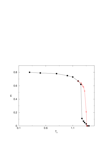
Figure 4: First-order transition with hysteresis for Ódor’s two-temperature Ising model. This and the last figure were kindly supplied by G. Ódor for this review.

Figure 5: Correlation and temperature $\langle T_{1}\rangle$ for negligible noise and various forgetting rates; $L=3001$. The lowest part shows one of the curves for longer times.

Figure 6: As Fig. 4, for various noise levels and a forgetting rate of 0.3 %. The curves for $T_{2}=0.2$ and 0.5 nearly overlap.

Figure 7: Correlations at $t=1000$, from previous figure, versus noise level.

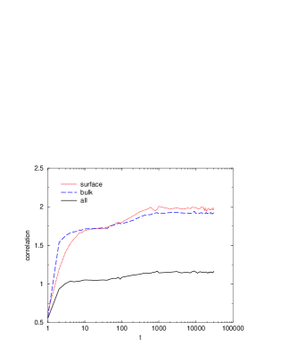
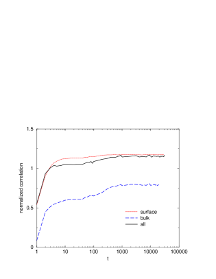
Figure 8: Noise $k_{B}T_{2}/J=2.5$ applied to surface sites only, to bulk sites only, and to both (left part). The right part applies a normalisation by the number of surface or bulk sites and shows that bulk noise reduces more strongly the segregation. 1 % forgetting, 0.003 tolerance steps.

As promised, now we introduce a second temperature $T_{2}$ in addition to the $T_{1}=T$ used above [21]. At each spin flip attempt, the spin flips if a random number is smaller than the above Glauber probability determined by the tolerance, or if another random number is smaller than the Glauber probability corresponding to the noise $T_{2}$. Thus both flips happen more often when the amount of unhappiness decreases more strongly, depending on exp($\Delta E/k_{B}T_{1}$) or exp($\Delta E/k_{B}T_{2}$), respectively. Such simulations were made first by Ódor [21] for spin 1/2 Ising models; noise lets the spontaneous magnetisation (= strength of long-range segregation) jump to zero, Fig.4 below. Also for our $Q=5$ Potts-like model and strong noise (x symbols in Fig. 2), segregation is strongly reduced, though in a continuous way. Fig.3 shows better the dependence on the strength $T_{2}$ of the noise.

Now we allow for individual temperatures $T_{1}(i)$ depending on the lattice site $i$. As discussed in the preceding section, at each iteration $T_{1}(i)$ increases by 0.01 if all four nearest neighbours belong to the same group as $i$, and it decreases by the same amount 0.01 if none of the four neighbours belong to the same group as $i$. In addition, at each iteration all $T_{1}$ are decreased by a small percentage, i.e. tolerance is slowly forgotten.

Fig.5 shows the resulting correlation $C$ and average temperature $T_{1}$ for negligible noise and various forgetting rates. Fig.6 shows the same two quantities for various noise levels at a forgetting rate of 0.3 percent. Fig.7 shows these results at the end of the simulation, $t=1000$, against the noise level $T_{2}$; for $T_{2}$ up to 1 the noise effects are nearly negligible, and above $T_{2}=5$ their effects are strong and nearly independent of $T_{2}$.

[For large $T_{2}$ we omitted the reduction of $T_{1}(i)$ by 0.01 since otherwise these temperatures became negative. Apparently for $Q>2$ the condition $n=0$ (none of my neighbours belongs to my group) occurs much more often than the opposite condition $n=4$ (all my neighbours belong to my group), and thus the previous changes by $\pm 0.01$ no longer balance each other. Thus we used only increases by 0.01 if $n=4$, balanced by the overall forgetting rate of 0.003.]

From Ódor’s simulations, Fig.8 distinguishes between the noise $T_{2}$ applied to the surface sites, to the bulk sites or to both. Its left part shows the lowest segregation if both surface and bulk sites are subjected to noise. However, its right part normalizes the functions by the number of surface and bulk sites, respectively, and then shows that bulk noise reduces segregation much more than surface noise. (Here, ”bulk” are the sites surrounded by four neighbours of the same group, and “surface” is the opposite case.)

Thus this section showed that a lot of external noise can perturb the personal preferences for neighbours of the same group. For two groups [21], there is a first-order phase transition at some critical noise level; for $Q=5$ there is no such sharp transition, neither as a function of $T_{1}$ nor as a function of $T_{2}$, but noise still can reduce appreciably the strength of segregation. This sounds trivial but for zero noise the Schelling and Ising models do not lead to large domains [9, 7, 8, 13]. Thus only small but nonzero noise can produce segregation into ghettos.

5 Summary

This review and the earlier publications from physicists [10, 11, 12, 7, 14, 21] tried to overcome the segregation between sociology and physics with regard to the possible self-organisation (“emergence”) of residential segregation in cities. Besides outside forces like racial discrimination, also personal preferences can lead to segregation, as pointed out by Schelling [4] through his Ising-like model. Whether this clustering leads to “infinitely” large domains (=ghettos) depends on details. The original Schelling model failed to give ghettos; with some randomness [9], neutral moves [7], or positive temperature [8] that can be repaired. Nevertheless, the inclusion of empty residences and the search for the nearest suitable residence make the Schelling model unnecessarily complicated, and the two-dimensional Ising model seems to be a suitable simplification, giving infinite domains for $0<T<T_{c}$.

Schelling not only asked the right question but also invented a model similar to those typically studied by physicists like the Ising model of 1925. Thus sociologist who like the Schelling model should not complain about physics models with up and down spins to be too unrealistic, and physicists studying up and down spins should not claim that they bring something very novel to sociology.

We thank S. Solomon, G. Ódor, K. Müller, W. Jentsch, W. Alt and S. Galam for cooperation and suggestions.

References

- [1] C. Castellano, S. Fortunato, V. Loreto, Statistical physics of social dynamics, arXiv:0710:3256, preprint for Rev. Mod. Phys.
- [2] R. Sethi, R. Somanathan, (2007). “Racial Income Disparities and the Measurement of Segregation: Evidence from the 2000 Census.” Unpublished Manuscript, Barnard College, Columbia University.
- [3] J. Friedrichs (1998) Urban Studies 35: 1745 (1998)
- [4] T.C. Schelling (1971) J. Math. Sociol. 1: 143; see also M. Fossett (2006) ibid. 30: 185; S. Benard, R. Willer (2007) ibid. 31: 149
- [5] W. Weidlich, Sociodynamics: A Systematic Approach to Mathematical Modelling in the Social Sciences (Gordon and Breach, London, 2000).
- [6] N.E. Aydinomat, A short interview with Thomas C. Schelling, Economics Bulletin 2, 1 (2005).
- [7] D. Vinkovic, A. Kirman (2006) Proc. Natl. Acad. Sci. USA 103: 19261
- [8] D. Stauffer, S. Solomon (2007), Eur. Phys. J. B 57: 473
- [9] E. Dethlefsen, C. Moody (July 1982) Byte 7: 178; F.L. Jones (1985) Aust. NZ J. Sociol. 21: 431
- [10] M. Levy, H. Levy and S. Solomon, Microscopic Simulation of Financial Markets, Academic Press, San Diego (2000).
- [11] H. Meyer-Ortmanns (2003) Int. J. Mod. Phys. C 14: 311
- [12] C. Schulze (2005) Int. J. Mod. Phys. C 16: 351
- [13] V. Spirin, P.L. Krapivsky and S. Redner (2001) Phys. Rev. E 63: 036118.
- [14] K. Müller, C. Schulze and D. Stauffer (2008) Int. J. Mod. Phys. C 19: issue 3.
- [15] L. Dall’Asta, C. Castellano and M. Marsili, eprint arXiv:0707.1681
- [16] J.J. Schneider, S. Kirkpatrick, Stochastic Optimization, Springer, Berlin, Heidelberg, New York, 2006.
- [17] J. Mimkes (1996) J. Thermal Anal. 43: 521.
- [18] D. Stauffer (2007) Am. J. Phys. 75, issue 11.
- [19] D. Stauffer, C. Hartzstein, K. Binder and A. Aharony (1984) Z. Physik B 55: 325.
- [20] M. A. Sumour, A.H. El-Astal, M.A. Radwan, M.M. Shabat (2008) preprint for Int. J. Mod. Phys. C 19.
- [21] G. Ódor (2008) Int. J. Mod. Phys. C 19, issue 11.