Anomalous shell effect in the transition from a circular to a triangular billiard

Abstract

We apply periodic orbit theory to a two-dimensional non-integrable billiard system whose boundary is varied smoothly from a circular to an equilateral triangular shape. Although the classical dynamics becomes chaotic with increasing triangular deformation, it exhibits an astonishingly pronounced shell effect on its way through the shape transition. A semiclassical analysis reveals that this shell effect emerges from a codimension-two bifurcation of the triangular periodic orbit. Gutzwiller’s semiclassical trace formula, using a global uniform approximation for the bifurcation of the triangular orbit and including the contributions of the other isolated orbits, describes very well the coarse-grained quantum-mechanical level density of this system. We also discuss the role of discrete symmetry for the large shell effect obtained here.

I Introduction

The periodic orbit theory (POT) is a very useful tool to study shell structure in single-particle energy spectra. In POT, the quantum-mechanical level density is semiclassically approximated in terms of the periodic orbits of the corresponding classical system. For systems with only isolated orbits, Gutzwiller derived the so-called “trace formula” Gutz which is particularly successful for chaotic systems. The POT for 3D cavities was developed in BB . In integrable systems, semiclassical trace formulae can be derived from torus quantization BerryTabor ; CrLit1 . However, most physical systems lie between the above two extreme situations, i.e., they exhibit mixed phase-space dynamics in which both regular and chaotic motion coexists on the same energy shell. For systems with various types of continuous symmetries, trace formulae have been derived in CrLit1 ; StruMa ; CrLit2 . For an introductory text book on semiclassical physics and applications of the POT to various physical systems, we refer to BrackText .

In both integrable and mixed systems, bifurcations of periodic orbits can significantly influence the shell structure. The above-mentioned semiclassical trace formulae, which are all based on the stationary-phase approximation (SPA), diverge when bifurcations of periodic orbits occur under variations of energy or potential parameters (e.g., deformations). In the SPA, the classical action integral is expanded around its stationary points (corresponding to periodic orbits) up to quadratic terms and the trace integral is evaluated in terms of Gauss-Fresnel integrals. At bifurcation points, the determinant of the coefficient matrix of the quadratic terms becomes zero and the Gauss-Fresnel integral becomes singular. In order to obtain a finite semiclassical level density near bifurcation points, higher-order expansion terms of the action integral are needed, which are most conveniently found from the normal forms appropriate to the types of bifurcation under consideration Ozorio ; Sie96 ; SchSie97 .

Quantum billiards (and their 3D versions, cavities), besides being quite useful toy models to study POT, reflect important features of finite physical quantum systems such as quantum dots, metallic clusters, and atomic nuclei. E.g., non-integrable 3D cavities with realistic shapes appropriate for fission barriers of actinide nuclei have been used in POT to explain the onset of the mass asymmetry of the nascent fission fragments fisasy . On the other hand, many integrable billiard systems are well known and fully understood semiclassically, e.g., circular, equilateral triangular, square, and elliptic billiards (cf. BrackText ), and may be used as simple models for physical systems. In these, bifurcations of short periodic orbits may lead to a considerable enhancement of shell effects. E.g., in the elliptic billiard, the short diametric orbit undergoes successive bifurcations with increasing deformation, and new periodic-orbit families emerge Sie96 ; Nishioka1 ; Magner99 . The same type of bifurcations occur for equatorial orbits in the 3D spheroidal cavity Nishioka2 and provide a schematic explanation of nuclear super-deformed and hyper-deformed shell structure ASM ; Magner02 . In these studies, it was shown that a system may turn strongly chaotic by adding small reflection-asymmetric (e.g., octupole) deformations SAM .

In this paper, we apply the POT to a two-dimensional non-integrable billiard system whose boundary is continuously varied from a circular to an equilateral triangular shape. This study is initiated to explore a possible quantum dot system. Many studies have been undertaken for quantum dots, but this type of deformation has not been studied before. Another important aim is to investigate the role of discrete symmetries. As will be discussed, the present model possesses the discrete $C_{3v}$ point-group symmetry. Recently, several mean-field studies of nuclei have suggested the possible existence of low-lying states with exotic shapes with point-group symmetries, such as tetrahedral and octahedral deformations Dudek . In order for such shapes to be stabilized, rather large quantum shell effects in the single-particle spectra are necessary. We will discuss the role of discrete symmetries in establishing strong shell effects.

II Shell Structure and Level Statistics

II.1 The model system

We consider the two-dimensional billiard system

$$H=\frac{\bm{p}^{2}}{2m}+V(\bm{r}),\qquad V(\bm{r})=\left\{\!\!\begin{array}[]{c@{\quad}l}0&r<R(\theta)\\ \infty&r>R(\theta)\end{array}\right.$$ (1)

in polar coordinates $\bm{r}=(r,\theta)$, whereby the boundary shape $R(\theta)$ is parameterized implicitly by the equation

$$R^{2}+\frac{2\sqrt{3\alpha}}{9}\frac{R^{3}}{R_{0}}\cos(3\theta)=R_{0}^{2}\,,\qquad\theta\in[0,2\pi)\,.$$ (2)

Figure 1 shows the shape of the boundary for several values of $\alpha$.

Figure 1: Shapes of the boundary given by Eq. (2) for several values of deformation parameter $\alpha$.

This system possesses the discrete symmetries of the point group $C_{3v}$, consisting of $\pm 2\pi/3$ rotations about the origin and reflections with respect to the three axes through the origin with $\theta=0,\pm\pi/3$. The deformation parameter $\alpha=0$ yields a circular shape and $\alpha=1$ an equilateral triangle. The system is integrable in these two limits, but non-integrable in between.

For the calculation of the quantum spectrum of this system, it is useful to decompose the wave functions into free circular waves:

$$\psi_{k}(r,\theta)=\sum_{m=-\infty}^{\infty}c_{m}J_{|m|}(kr)e^{im\theta},$$ (3)

where $k=\sqrt{2me}/\hbar$ is the wave number and $e$ the energy.

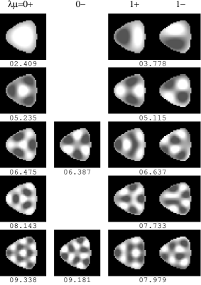
Figure 2: Wave functions of some lowest eigenstates for $\alpha=0.4$. $0+$, $0-$ and $1\pm$ are states of type (5a), (5b) and (5c’), respectively. Their $k$ values are also indicated.

Taking the $C_{3v}$ symmetry into account, we can classify the eigenstates according to the eigenvalues of the symmetry operators

$$\mathcal{R}\psi^{(\lambda\mu)}=e^{2\pi i\lambda/3}\psi^{(\lambda\mu)},$$ (4a)

$$\mathcal{P}\psi^{(\lambda\mu)}=(-1)^{\mu}\psi^{(\lambda\mu)},$$ (4b)

where $\mathcal{R}$ and $\mathcal{P}$ represent rotation by $2\pi/3$ around the origin and reflection with respect to the $x$ axis, respectively. We have simultaneous eigenstates of $\mathcal{R}$ and $\mathcal{P}$ for $\lambda=0$ states, and then we can classify the eigenstates into four sets, which correspond to the irreducible representations (“irreps”) of the $C_{3v}$ point group LandauQM :

$$\psi_{k}^{(0+)}(r,\theta)=\sum_{m=0}^{\infty}c_{m}^{(0+)}J_{3m}(kr)\cos(3m\theta)\,,$$ (5a)

$$\psi_{k}^{(0-)}(r,\theta)=\sum_{m=1}^{\infty}c_{m}^{(0-)}J_{3m}(kr)\sin(3m\theta)\,,$$ (5b)

$$\psi_{k}^{(\pm 1)}(r,\theta)=\sum_{m=-\infty}^{\infty}c_{m}^{(\pm 1)}J_{|3m\pm 1|}(kr)e^{i(3m\pm 1)\theta}.$$ (5c)

$\psi_{k}^{(+1)}$ are the complex conjugates of $\psi_{k}^{(-1)}$, and the two form degenerate pairs of states. (The point group $C_{3v}$ has two 1-dimensional irreps and one 2-dimensional irrep. The states $(0\pm)$ correspond to the 1-dimensional irreps, and the degenerate pairs of states $(\pm 1)$ correspond to the 2-dimensional irrep.) Taking linear combinations of these, one finds the following alternative real expressions for the states (5c):

$$\psi^{(1\pm)}_{k}(r,\theta)=\!\!\sum_{m=-\infty}^{\infty}\!\!\!c_{m}^{(1\pm)}J_{|3m+1|}(kr)\left\{\begin{array}[]{c}\cos((3m+1)\theta)\\ \sin((3m+1)\theta)\end{array}\right\}\!,$$

(5c’)

which are not eigenstates of the operator $\mathcal{R}$, but of the operator $\mathcal{P}$. The eigenvalue spectrum $\{k_{n}\}$ and the coefficients $c_{m}$ are determined by the Dirichlet boundary condition $\psi_{k_{n}}(R,\theta)=0$. We show some eigenfunctions in Fig. 2. The states belonging to the sets (5a) and (5b) have symmetry under the rotation $\mathcal{R}$. The former are even under the reflection $\mathcal{P}$, while the latter are odd.

Figure 3 shows the lower part of the energy spectrum $\{e_{n}\}=\{\hbar^{2}k_{n}^{2}/2m\}$, plotted against the deformation parameter $\alpha$.

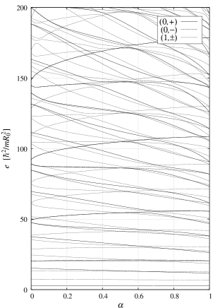
Figure 3: Lowest part of energy spectrum (in units of $\hbar^{2}\!/mR_{0}^{2}$), plotted against the deformation parameter $\alpha$.

We note that the levels bunch into small energy intervals in the region $\alpha\simeq 0.5-0.7$, forming large gaps in the spectrum. It is, in fact, quite surprising to realize that the shell gaps in this non-integrable region are much larger than in the two integrable limits $\alpha=0$ and $\alpha=1$.

Figure 4: Scaled shell-correction energy $\delta E(N)$ (in units of $\hbar^{2}/mR_{0}^{2}$) versus $\sqrt{N}$.

The gaps cause large shell effects in the total energy of a system of $N$ noninteracting fermions described by the Hamiltonian (1). We split the energy into a smooth and an oscillating part

$$E(N)=2\sum_{n=1}^{N/2}e_{n}=\bar{E}(N)+\delta E(N)\,,\quad(N\hbox{ even})$$ (6)

whereby the factor 2 accounts for the spin $s=1/2$. The smooth part $\bar{E}(N)$ is equivalently given by a Strutinsky averaging strut , the extended Thomas-Fermi model, or the Weyl expansion (cf. BrackText , Ch. 4), while the shell-correction energy $\delta E(N)$ reflects the quantum effects; it is dominated by the shortest periodic orbits of the classical system as demonstrated below for the case of the level density. Large gaps in the spectrum lead to large amplitudes of $\delta E(N)$. This is demonstrated in Figure 4 where we present $\delta E(N)$, scaled by a factor $\sqrt{N}$, for three values of $\alpha$. We note that the oscillatory pattern for $\alpha=0.5$ is quite regular and on the average has a much larger amplitude than in the integrable limits.

II.2 Level statistics

Nearest-neighbor spacing (NNS) distributions are commonly used to identify signatures of chaos in a quantum system. Generically, classically chaotic systems exhibit level repulsion and the NNS distributions are of Wigner type, while regular systems typically have degeneracies and the NNS distributions are Poisson like BoGiSch . To extract these universal fluctuation properties, one has to use unfolded spectra whose mean level density is normalized to unity. Thus, for systems with discrete symmetries, one has to study the NNS of the subsets of levels belonging to the irreps of the corresponding point group.

The average total level density of a two-dimensional billiard is given by Weyl’s asymptotic formula Weyl

$$\bar{g}(e)\sim\frac{m}{2\pi\hbar^{2}}\,A+{\cal O}(e^{-1/2})\,,$$ (7)

in which the leading-order term is proportional to the area $A$ surrounded by the boundary and does not depend on the energy. This means that for large energies $e$ the mean level spacing $\bar{\Delta}$ becomes asymptotically constant:

$$\bar{\Delta}\;\longrightarrow\;\bar{\Delta}_{0}=\frac{1}{\bar{g}}\sim\frac{2\pi\hbar^{2}}{mA}\,.$$ (8)

As discussed in the previous subsection, the quantum levels of our system fall into four sets $\{e_{n}^{\kappa}\}$ with $\kappa=0\pm$ and $\pm 1$, corresponding to the eigenstates (5a,b) and (5c) or (5c’), respectively. The numbers of levels in these sets have the relative ratios

$$N^{(0+)}:N^{(0-)}:N^{(+1)}:N^{(-1)}=1:1:2:2\,,$$

and hence the mean level spacing in each set is given by

$$\bar{\Delta}^{(0\pm)}=6\bar{\Delta}_{0}\,,\qquad\bar{\Delta}^{(\pm 1)}=3\bar{\Delta}_{0}\,.$$ (9)

The unfolded level spacings are then obtained by

$$s_{n}^{(\kappa)}=\frac{e_{n+1}^{(\kappa)}-e_{n}^{(\kappa)}}{\bar{\Delta}^{(\kappa)}}\,.\qquad(\kappa=0\pm,\pm 1)$$ (10)

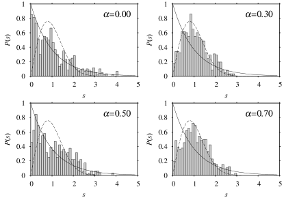
Figure 5: Nearest-neighbor spacing distribution $P(s)$ for four values of the deformation parameter $\alpha$. The lowest 600 levels (i.e., 100 and 200 levels of the subsets $0\pm$ and $\pm 1$, respectively) were used to obtain the statistics. Solid and dashed lines show Poisson and Wigner distributions, respectively.

Figure 6: Brody parameter $\omega$ for nearest-neighbor spacing distribution, plotted as a function of $\alpha$.

Figure 5 shows the NNS distributions $P(s)$, averaged over all four sets. At $\alpha=0$, the system is integrable and the distribution is Poisson like as expected. At $\alpha=0.3$, the distribution changes into Wigner form. A similar situation is also found at $\alpha=0.7$. At $\alpha=0.5$, however, the distribution deviates considerably from the Wigner form and becomes closer to a Poisson distribution. For mixed systems, the NNS distributions $P(s)$ are often fitted by a Brody distribution Brody

$$B(s,\omega)=\beta(\omega+1)s^{\omega}\exp(-\beta s^{\omega+1}),\quad\beta=\left[\Gamma\!\left(\tfrac{\omega+2}{\omega+1}\right)\right]^{\omega+1}$$ (11)

which interpolates between the Poisson ($\omega=0$) and Wigner ($\omega=1$) distributions. The Brody parameter $\omega$ can then be taken as a measure for the chaoticity of NNS distribution. In Figure 6 we show $\omega$ as obtained by fitting the $P(s)$ distributions of Fig. 5 to (11). We clearly recognize two peaks around $\alpha\simeq 0.3$ and $\simeq 0.7$, exhibiting near-chaoticity, separated by a deep minimum around $\alpha\simeq 0.5$ where the system appears to approach regularity. As we will discuss below, this near-regularity is related to an approximate restoration of local dynamical symmetry due to a periodic-orbit bifurcation.

III Fourier Analysis and Classical Periodic Orbits

In the POT, the quantum level density $g(e)$ is approximated in terms of classical periodic orbits by the semiclassical trace formula Gutz ; BB ; BerryTabor ; StruMa ; CrLit1 ; CrLit2

$$g(e) =\sum_{n}\delta(e-e_{n})$$

$$\simeq\bar{g}(e)+\sum_{\xi}A_{\xi}(e)\cos\left(\frac{S_{\xi}(e)}{\hbar}-\frac{\pi}{2}\nu_{\xi}\right)\!,~{}~{}$$ (12)

where the first term, like for the energy in (6), represents the smooth part, while the second term contains the quantum shell effects. In the latter, the sum is taken over all periodic orbits $\xi$ of the classical system (or the orbit families $\xi$ in systems with continuous symmetries BerryTabor ; StruMa ; CrLit1 ), $S_{\xi}$ is the action integral around $\xi$, and $\nu_{\xi}$ is the Maslov index CrRoLi ; Sugita . The amplitude $A_{\xi}$ depends on the stability of the orbit $\xi$ (and, for an orbit family, on the phase-space volume covered by the family). For isolated orbits, the amplitude $A_{\xi}$ was given by Gutzwiller Gutz :

$$A_{\xi}(e)=\frac{1}{\pi\hbar}\,\frac{T_{\xi}(e)}{\sqrt{|\det[1-M_{\xi}(e)]|}},$$ (13)

where $T_{\xi}(e)={\rm d}S_{\xi}(e)/{\rm d}e$ is the period of the orbit and $M_{\xi}(e)$ its stability matrix defined below. If an orbit has a discrete degeneracy $f$ (i.e., if there exist $f$ replicas with identical actions, stabilities and Maslov indices but different orientations) due to discrete symmetries, it has to be included $f$ times into the sum in (12). This holds also for time-reversed rotational orbits.

Transforming variables from energy $e$ to wave number $k$ and using the relation $S_{\xi}=\hbar kL_{\xi}$ for billiards, where $L_{\xi}$ is the length of the orbit $\xi$, the trace formula becomes

$$g(k) =\frac{\hbar^{2}k}{m}g(e)$$

$$\simeq\bar{g}(k)+\sum_{\xi}A_{\xi}(k)\cos(kL_{\xi}-\frac{\pi}{2}\nu_{\xi})\,.$$ (14)

Let us now consider the Fourier transform of the level density $g(k)$ with respect to $k$:

$$F(L)=\int_{-\infty}^{\infty}g(k)e^{-ikL}e^{-(k\Delta)^{2}/2}{\rm d}k.$$ (15)

The Gaussian damping factor is included for the truncation of the high-energy part of the spectrum. If we insert Eq. (14) and ignore the $k$ dependence of the amplitude factors $A_{\xi}$ (which are constant for isolated orbits in billiards and cavities), we obtain

$$F^{\rm sc}(L)=F_{0}(L)+\pi\sum_{\xi}e^{-i\pi\nu_{\xi}/2}A_{\xi}\,\delta_{\Delta}(L-L_{\xi})\,.$$ (16)

$\delta_{\Delta}(x)$ is a normalized Gaussian of width $\Delta$, which turns into Dirac’s delta function in the limit $\Delta\to 0$. Eq. (16) indicates that the Fourier transform $F(L)$ is a function with successive peaks at the lengths of the periodic orbits $L=L_{\xi}$, with heights proportional to the amplitudes $A_{\xi}$. We can therefore extract information about the classical periodic orbits from the Fourier transform of the quantum-mechanical level density:

$$F^{\rm qm}(L)=\sum_{n}e^{-ik_{n}L-(k_{n}\Delta)^{2}}\!,\quad k_{n}=\sqrt{2me_{n}}/\hbar\,.$$ (17)

Figure 7 shows the modulus of this Fourier transform of our system versus the deformation parameter $\alpha$. At $\alpha=0$, where the periodic orbits form degenerate families corresponding to rational tori, we find the peaks at the well-known orbit lengths of the circular billiard BB

$$L_{vw}=2vR_{0}\sin(w\pi/v)\,.$$ (18)

Here $w$ and $v$ are the winding number around the origin and the number of vertices $(v\geq 2w)$ of each orbit, respectively. For instance, $L=4R_{0}$ for the diametric orbit $(w=1,v=2)$, $L=3\sqrt{3}R_{0}$ for the triangular orbit $(w=1,v=3)$, $L=4\sqrt{2}R_{0}$ for the square orbit $(w=1,v=4)$, and so on. With increasing $\alpha$, we observe a dramatic enhancement of the peak height corresponding to the triangular orbit, $L\simeq 5.2R_{0}$ (and its second repetition, $L\simeq 10.4$), starting around $\alpha\simeq 0.4$ and culminating around $\alpha\simeq 0.55$. As we shall see below, this can be traced back to a codimension-two bifurcation of the triangular orbit.

Figure 7: Modulus $|F^{\rm qm}(L)|$ of Fourier transform of the quantum-mechanical level density versus deformation parameter $\alpha$.

In fact, for $\alpha>0$ all rational tori of the circular billiard are broken into pairs of stable and unstable isolated orbits. With increasing $\alpha$, bifurcations of the stable orbits occur and new periodic orbits emerge, which makes the phase-space increasingly chaotic. In the following, we first demonstrate this for the two shortest orbits and then focus on the triangular orbit.

The stability of a periodic orbit is described by the stability matrix $M_{\xi}$, which is defined by the linearized Poincaré map around the periodic orbit

$$M_{\xi}=\frac{\partial(\bm{q}(T_{\xi}),\bm{p}(T_{\xi}))}{\partial(\bm{q}(0),\bm{p}(0))},$$ (19)

where $(\bm{q}(t),\bm{p}(t))$ are the coordinates and momenta perpendicular to the periodic orbit $\xi$ as functions of time $t$, and $T_{\xi}$ is the period of the orbit. In a two-dimensional autonomous Hamiltonian system $M_{\xi}$ is a symplectic (2x2)-matrix, and the stability of a orbit is easily identified by looking at its trace $\mathop{\rm Tr}M_{\xi}$. For elliptic (stable) orbits, the eigenvalues of $M_{\xi}$ are of the form $(e^{iv},e^{-iv})$ with real $v\geq 0$, and thus $-2\leq\mathop{\rm Tr}M_{\xi}\leq 2$. For direct- and inverse-hyperbolic (unstable) orbits, the eigenvalues are $(e^{u},e^{-u})$ and $(-e^{u},-e^{-u})$, respectively, with real $u>0$, and hence $\mathop{\rm Tr}M_{\xi}>2$ and $\mathop{\rm Tr}M_{\xi}<-2$. Bifurcations of isolated orbits occur whenever $\mathop{\rm Tr}M_{\xi}=+2$.

Figure 8: Trace of stability matrix $\mathop{\rm Tr}M_{\xi}$ for the diameter orbits (2A) and the second repetition of the stable diameter orbit (2A²), plotted versus deformation parameter $\alpha$.

Figure 9: Same as Fig. 8 but for the triangular orbits, in the upper panel plotted versus $\sqrt{\alpha}$. The lower panel shows a magnification around the bifurcation of the stable orbit 3A occurring near $\alpha\simeq 0.407$.

Figures 8 and 9 show $\mathop{\rm Tr}M_{\xi}(\alpha)$ for the two shortest pairs of periodic orbits in our system. In Fig. 8, the stable branch (2A) of the diametric orbit is seen to undergo a period-doubling pitchfork bifurcation at $\alpha=0.166$, where a symmetric wedge-shaped orbit (4V) emerges. The latter undergoes a further pitchfork bifurcation at $\alpha=0.227$, where a pair of asymmetric wedge-shaped orbits (4U) emerges.

The bifurcation scenario of the triangular orbits is more complicated. In the upper panel of Fig. 9, where $\mathop{\rm Tr}M_{\xi}$ is plotted against $\sqrt{\alpha}$, the stable triangular orbit (3A) is seen to touch the critical line $\mathop{\rm Tr}M_{\xi}=+2$ near $\sqrt{\alpha}\simeq 0.63$ ($\alpha\simeq 0.4$) and to remain stable on either side. A pair of new stable (3D) and unstable (3C) triangular orbits emerge from the touching point. A magnification of the situation around $\alpha\simeq 0.4$, shown in the lower panel against $\alpha$, reveals that the scenario consists of two connected near-lying bifurcations, also called a “codimension-two bifurcation”. At $\alpha=0.400$, a tangent (saddle-node) bifurcation occurs, at which the new orbits 3D and 3C are born. Shortly after this bifurcation, the (old) stable orbit 3A and the new unstable orbit 3C encounter in a touch-and-go bifurcation at $\alpha=0.407$ (see Appendix A for its analytic value). Note that the new 3C and 3D orbits do not possess $C_{3v}$ symmetry, in contrast to the old 3A orbit, so that they occur in degenerate triplets obtained by successive rotations about $2\pi/3$, i.e., these orbits have a discrete degeneracy of $f=3$.

Figure 10: Poincaré surfaces of section $(\theta,\sin\varphi)$ in the fundamental domain of the $C_{3}$ group, plotted for several values of $\alpha$ (given at the upper left of each panel) in the bifurcation region of the triangular orbit 3A. $\theta$ is the polar angle of a reflection point and $\varphi$ the reflection angle measured from the normal to the boundary; the set $(\theta,\sin\varphi)$ is approximately area preserving.

Figure 10 shows excerpts of Poincaré surfaces of section $(\theta,\varphi)$ in the relevant regions. Here $\theta$ is the polar angle of a reflection point of an orbit at the boundary, while $\varphi$ represents the reflection angle measured from the normal to the boundary at the reflection point. The three upper panels illustrate the tangent bifurcation of the 3C and 3D orbits. For $\alpha=0.390$ (upper left), one sees one major regular island corresponding to the stable equilateral triangular orbit 3A. It contains its fixed point at $(\theta,\varphi)=(0,\pi/6)$, surrounded by quasi-tori (small aperiodic perturbations of the 3A orbit). At the bifurcation point $\alpha\approx 0.400$ (upper center), three cusps are formed by one of the surrounding quasi-tori in the island, and for $\alpha=0.401$ (upper right), the three stable fixed points of the new 3D orbits, surrounded by small regular islands, are seen to have emerged from each of the three cusps in the major island. The three saddles separating these three islands from the central island contain the unstable fixed points of the 3C orbits. The stable fixed point of the 3A orbit still persists at the original position at the center of the major island. The number $f=3$ of the new stable and unstable fixed points in the island is due to the three-fold discrete degeneracy of the orbits 3D and 3C mentioned above.

The lower three panels in Fig. 10 illustrate the touch-and-go bifurcation of the orbits 3A and 3C. At the bifurcation point $\alpha=0.407$ (lower left), the three unstable fixed points of the 3C orbits have contracted into a star-like intersection of three quasi-tori, located at the central fixed point $(\theta,\varphi)=(0,\pi/6)$ of the 3A orbit. The three nearby stable fixed points in the major island belong to the orbits 3D. For $\alpha=0.420$ (lower center), small stable islands have formed again around the fixed points of the 3A orbit, and nearby we recognize the three unstable fixed points of the 3C orbit. For $\alpha=0.500$ (lower right), the central island of the 3A orbits have grown, the three islands of the stable 3D orbits have shrunk, and the three unstable fixed points of the 3C orbits are about to be buried in the increasing chaotic structure.

The bifurcation of the triangular orbit 3A occurs at the deformation where we observed the onset of the large Fourier peak in Fig. 7. It is due to the appearance of the pair of six-fold degenerate new orbits 3D and 3C. In particular, the stable one (3D), besides the doubly-degenerate 3A orbit, adds to the local regularity of the phase space observed in Figs. 5, 7 and 10. It is therefore apparent that this bifurcation is responsible for the remarkable shell structure in the quantum spectrum seen in Fig. 3. Note that the maximum of the Fourier peak in Fig. 7 occurs at $\alpha\simeq 0.55$, i.e., above the bifurcation where the new orbits are born. The fact that the signature of a bifurcation is strongest after the bifurcation point (on the side where the new orbits exist) is a rather general trend for shell effects which can also be understood in terms of semiclassical uniform approximations Sie96 ; SchSie97 (see the following section and Fig. 13 below). It has also been observed recently in the level statistics of a Hamiltonian system with mixed phase space Marta .

IV Semiclassical Analysis

IV.1 Semiclassical level density near bifurcations

As mentioned above, the Gutzwiller trace formula (12) with the amplitudes (13) for isolated orbits diverges at bifurcation points. This is due to the break-down of stationary phase approximation, and higher-order terms in the expansion of the action integral must be included in the derivation of the trace formula. For this purpose, it is necessary Ozorio to express the trace integral in phase space. After integrating over the coordinate and momentum parallel to an isolated orbit $\xi$ in a two-dimensional system, its semiclassical contribution to the oscillating part of the level density becomes CrLit1 ; SchSie97 ; Magner02

$$\delta g_{\xi}(e)= \frac{1}{2\pi^{2}\hbar^{2}}\mathop{\rm Re}\int_{-\infty}^{\infty}{\rm d}q^{\prime}\int_{-\infty}^{\infty}{\rm d}p\,\frac{1}{n_{r}}\,\frac{\partial\widehat{S}}{\partial e}\,\left|\frac{\partial^{2}\widehat{S}}{\partial p\partial q^{\prime}}\right|^{1/2}$$

$$\times\exp\!\left[\frac{i}{\hbar}\widehat{S}(q^{\prime},p)-\frac{i}{\hbar}q^{\prime}p-\frac{i\pi}{2}\nu_{\xi}\right].$$ (20)

Here $q^{\prime}$ is the final coordinate and $p$ the initial momentum perpendicular to the orbit $\xi$, the two forming a canonical pair of variables $(q^{\prime},p)$ to describe the “natural” Poincaré surface of section (PSS) of the orbit on which $(q^{\prime},p)=(0,0)$ is its fixed point. For generic bifurcations, $n_{r}$ is the repetition number of the primitive orbit. The function $\widehat{S}(q^{\prime},p)$ denotes the Legendre transform of $S(q^{\prime},q)$:

$$\widehat{S}(q^{\prime},p)=S(q^{\prime},q)+q^{\prime}p\,,$$ (21)

where $S(q^{\prime},q)$ is the (open) action integral along the orbit $\xi$ (at fixed energy $e$)

$$S({\bm{r^{\prime}},\bm{r})=\int_{\bm{r^{\prime}}}^{\bm{r}}{\bm{p}}_{\xi}(\bm{r}^{\prime\prime}})\cdot{\rm d}\bm{r^{\prime\prime}},$$ (22)

projected on the $q$ axis. The function $\widehat{S}(q^{\prime},p)$ is actually the generating function of the Poincaré map:

$$\widehat{S}(q^{\prime},p):\quad(q,p)\rightarrow(q^{\prime},p^{\prime})\,.$$ (23)

If one expands the function $\Phi(q^{\prime},p)=\widehat{S}(q^{\prime},p)-q^{\prime}p$ in the phase of the integrand of (20) around $q^{\prime}=p=0$ up to quadratic terms in $q^{\prime}$ and $p$ and evaluates the integrals in (20) by the standard stationary phase approximation (SPA), one obtains the contribution of the orbit $\xi$ to Gutzwiller’s trace formula (12) with the amplitude (13). Near bifurcations of the orbit $\xi$, the SPA breaks down and one has to include higher-order terms in the expansion of $\Phi(q^{\prime},p)$. The minimum number of terms needed to describe a given bifurcation scenario on the PSS leads to the so-called “normal forms” of $\Phi(q^{\prime},p)$, which depend on the type of bifurcation. Doing the integrations in (20) using such normal forms leads to a finite combined contribution of the orbit $\xi$ and all the orbits involved in its bifurcation to the trace formula. In order to conform with standard notation, we rename the function $\Phi(q^{\prime},p)$ by $S(q^{\prime},p)$ which, according to (21), is identical with the projected action integral $S(q^{\prime},q)$, but taken as a function of the variables $q^{\prime}$ and $p$.

IV.2 Normal form for codimension-two bifurcation

For the description of the codimension-two bifurcation scenario of the orbit 3A and its satellites 3C, 3D discussed in the previous section and illustrated on the PSS in Fig. 10, the following normal form is appropriate Schom97 :

$$S(I,\varphi)=S_{0}(\alpha)-\epsilon I-aI^{3/2}\cos(3\varphi)-bI^{2}\,.$$ (24)

Here one has transformed the Poincaré variables $(q^{\prime},p)$ to quasi-polar variables $(I,\varphi)$ by

$$p=\sqrt{2I}\cos\varphi\,,\qquad q^{\prime}=\sqrt{2I}\sin\varphi\,.$$ (25)

In (24), $S_{0}(\alpha)$ is the (closed) action integral of the central (3A) orbit as a function of $\alpha$. The “bifurcation parameter” $\epsilon$ is a monotonously decreasing function of $\alpha$ such that $\epsilon=0$ at the touch-and-go bifurcation point (here $\alpha=\alpha_{0}=0.407$) of the central orbit, and that $\epsilon<0$ for $\alpha>\alpha_{0}$. $a$ and $b$ are parameters which are specific for the system and will be determined below.

That (24) is able to describe the correct fixed-point structure not only of the 3A orbit but also of its satellites 3C and 3D, will now be shown explicitly. We first rewrite (24) in terms of $q^{\prime}$ and $p$:

$$S(q^{\prime},p)=S_{0}-\frac{\epsilon}{2}(p^{2}+q^{\prime 2})-\frac{a}{\sqrt{8}}(p^{3}-3pq^{\prime 2})-\frac{b}{4}(p^{2}+q^{\prime 2})^{2}.$$ (26)

The stationary-phase conditions are

$$\frac{\partial S}{\partial q^{\prime}}\Bigr{|}_{q_{i}}=0\,,\qquad\frac{\partial S}{\partial p}\Bigr{|}_{p_{i}}=0\,.$$ (27)

One of the solutions is $q_{0}=0$, $p_{0}=0$ and corresponds to the central 3A orbit. This is so by default, due to the choice of the Poincaré variables $(q,p)$. Two further stationary points are found to be

$$q_{1,2}=0\,,\qquad p_{1,2}=-\frac{3a}{4\sqrt{2}\,b}\pm\sqrt{\frac{9a^{2}}{32b^{2}}-\frac{\epsilon}{b}}\,.$$ (28)

The fixed points $(q_{i},p_{i})$ with $i=1,2$ belong to the satellite orbits 3C and 3D, respectively. Two more pairs of fixed points for each of them are found by rotations in the $(I,\varphi)$ plane: $\varphi\to\varphi\pm 2\pi/3$. $\epsilon_{1}=9a^{2}\!/32b$ is the critical value for $p_{1,2}$ to have real values, i.e., for the real orbits 3C and 3D to exist. For our system we can choose $b>0$, and therefore $\epsilon_{1}>0$. For $\epsilon>\epsilon_{1}$, the orbits 3C and 3D become imaginary and only the central orbit 3A is real. With decreasing $\epsilon$, the three pairs of stable and unstable satellite orbits appear at $\epsilon=\epsilon_{1}$ which we identify with the tangent bifurcation point. At $\epsilon=0$ we have the touch-and-go bifurcation as stated above. For $\epsilon<0$ ($\alpha>\alpha_{0}$), all orbits are real.

The normal-form parameters $\epsilon$, $a$ and $b$ can be determined by fitting the actions $S$ and stability traces $\mathop{\rm Tr}M$ of the orbits, which have been obtained numerically, to their local behaviors predicted by the normal form (24). The stability trace is given in terms of $\widehat{S}$ by SchSie97

$$\mathop{\rm Tr}M=\left(\!\frac{\partial^{2}\widehat{S}}{\partial p\partial q^{\prime}}\!\right)^{\!\!-1}\!\left[1+\left(\!\frac{\partial^{2}\widehat{S}}{\partial p\partial q^{\prime}}\!\right)^{\!\!2}\!\!-\frac{\partial^{2}\widehat{S}}{\partial p^{2}}\frac{\partial^{2}\widehat{S}}{\partial{q^{\prime}}^{2}}\right]\!\!.$$ (29)

For the central orbit, it becomes

$$\mathop{\rm Tr}M_{0}=\mathop{\rm Tr}M_{A}=2-\epsilon^{2}\,,$$ (30)

so that $\epsilon$ can be determined as $\epsilon=\pm\sqrt{2-\mathop{\rm Tr}M_{A}}$, choosing the correct sign on either side of the bifurcation. The other parameters are obtained from the action difference of the satellite orbits 1 and 2 (i.e., 3C and 3D). Inserting $(q_{1,2},p_{1,2})$ from (28) into (26), one finds

$$\frac{S_{D}-S_{C}}{\hbar kR_{0}}=\frac{4}{3b}\sqrt{\epsilon_{1}}(\epsilon-\epsilon_{1})^{3/2}.$$ (31)

By fitting the numerical data for $S_{D}-S_{C}$ as function of $\epsilon$, we obtain $\epsilon_{1}$ and $b$, and therefore $a$. Thus we can uniquely determine all the normal form parameters. The results for the triangular orbits discussed above are

$$a=\frac{0.519252}{\sqrt{\hbar kR_{0}}}\,,\;\,b=\frac{2.34950}{\hbar kR_{0}}\,,\;\,\epsilon_{1}=0.0322755\,.$$ (32)

The formulae for the stability traces for the orbits 3C and 3D are

$$\mathop{\rm Tr}M_{C,D} =2\pm 12\sqrt{\epsilon_{1}^{3}(\epsilon_{1}-\epsilon)}-24\epsilon_{1}(\epsilon_{1}-\epsilon)$$

$$\quad\pm 12\sqrt{\epsilon_{1}(\epsilon_{1}-\epsilon)^{3}}\,,$$ (33)

and the action difference between orbits 3C and 3A is

$$\frac{S_{C}-S_{A}}{\hbar kR_{0}}=\frac{1}{12b}\!\left[\,3\epsilon^{2}\!-12\epsilon_{1}\epsilon+8\epsilon_{1}^{2}\!-8\sqrt{\epsilon_{1}(\epsilon_{1}-\epsilon)^{3}}\,\right]\!.$$ (34)

We have checked that the numerical results in the neighborhood of the bifurcations are nicely reproduced by these equations.

IV.3 Uniform approximations

Inserting the normal form (24) into the integral (20), one obtains a “local” uniform approximation Ozorio which is finite and valid near the bifurcation, i.e., for not too large absolute values of $\epsilon$. Due to the $C_{3v}$ symmetry of our system, the touch-and-go bifurcation is non-generic and isochronous. The factor $n_{r}$ in the denominator of (20) here must be chosen note as $n_{r}=f=3$. We have another degeneracy factor 2 in the numerator due to the time-reversal symmetry of all orbits. Using the variables $(I,\varphi)$ and changing the energy $e$ to the wave number $k$, we finally obtain the following expression for the local uniform approximation, in which the integration over $\varphi$ can be done analytically:

$$\delta g_{\xi}(k)=\frac{1}{3\pi^{2}\hbar}\,\mathop{\rm Re}\int_{0}^{\infty}{\rm d}I\int_{0}^{2\pi}{\rm d}\varphi\,L_{\xi}\left|\frac{\partial^{2}\widehat{S}}{\partial I\partial\varphi}\right|^{1/2}$$

$$\times\exp\left[\frac{i}{\hbar}\!\left\{S_{0}-I\varphi-\epsilon I-aI^{3/2}\cos(3\varphi)-bI^{2}\right\}-\frac{i\pi}{2}\nu_{\xi}\right]$$

$$=\frac{2L_{\xi}}{3\pi\hbar}\mathop{\rm Re}e^{ikL_{\xi}-i\pi\nu_{\xi}/2}\!\!\int_{0}^{\infty}\!\!{\rm d}I\,J_{0}(\tfrac{a}{\hbar}I^{3/2})e^{\frac{i}{\hbar}(-\epsilon I-bI^{2})}.$$ (35)

The integration over $I$ can be performed numerically using an expansion formula given in Schom97 .

As stated above, the result (35) is only useful in the neighborhood of the bifurcation. Far away from it, where all involved orbits become isolated, it can be evaluated asymptotically (corresponding to the SPA), but the amplitudes of the orbits then do not agree with the Gutzwiller values (13). In order to achieve this, one must develop “global” uniform approximations Sie96 ; SchSie97 . To that purpose, one needs to include higher-order expansion terms in the normal form. For the codimension-two bifurcation of our type one obtains, after suitable coordinate transformations Schom98 ,

$$\delta g_{\xi}(k)=\frac{1}{3\pi^{2}\hbar}\mathop{\rm Re}\int_{0}^{\infty}{\rm d}I\int_{0}^{2\pi}{\rm d}\varphi\,\Psi(I,\varphi)$$

$$\times\exp\left[\frac{i}{\hbar}\left\{S_{0}-I\varphi\!-\epsilon I-aI^{3/2}\cos(3\varphi)-bI^{2}\right\}-\frac{i\pi}{2}\nu_{\xi}\right]$$ (36)

with

$$\Psi(I,\varphi)=L_{\xi}-\alpha I-\beta I^{3/2}\cos(3\varphi),$$ (37)

where $\alpha$ and $\beta$ are expressed by a certain combination of higher-order expansion coefficients. In practice, these parameters are determined such that (36) yields the sum of contributions with amplitudes (13) of all involved isolated orbits far away from the bifurcation point. They are determined by equating (cf. Kaidel2 )

$$\frac{L_{C}}{\sqrt{|2-\mathop{\rm Tr}M_{C}|}}=\frac{L_{A}-\alpha I_{C}-\beta I_{C}^{3/2}}{\sqrt{|\det\Phi^{\prime\prime}(I_{C})|}}\,,$$ (38)

$$\frac{L_{D}}{\sqrt{|2-\mathop{\rm Tr}M_{D}|}}=\frac{L_{A}-\alpha I_{D}-\beta I_{D}^{3/2}}{\sqrt{|\det\Phi^{\prime\prime}(I_{D})|}}\,,$$ (39)

with

$$\det\Phi^{\prime\prime}=\begin{vmatrix}\frac{\partial^{2}S}{\partial{\varphi}^{2}}&\frac{\partial^{2}S}{\partial\varphi\partial I}\\ \frac{\partial^{2}S}{\partial I\partial\varphi}&\frac{\partial^{2}S}{\partial I^{2}}\end{vmatrix}_{\varphi=0}=\begin{vmatrix}\frac{\partial^{2}S}{\partial{q^{\prime}}^{2}}&\frac{\partial^{2}S}{\partial q^{\prime}\partial p}\\ \frac{\partial^{2}S}{\partial p\partial q^{\prime}}&\frac{\partial^{2}S}{\partial p^{2}}\end{vmatrix}_{q^{\prime}=0}\!\!\!,$$ (40)

and

$$I_{C,D}=\frac{1}{2}\left(q_{1,2}^{2}+p_{1,2}^{2}\right).$$ (41)

We now have all ingredients ready for calculating the semiclassical level density of our system. Since it is well-known Gutz that the sum over all periodic orbits does not converge in systems with mixed dynamics, we have to introduce a certain truncation. This is achieved BrackText ; SieSt by focusing on the gross-shell structure of the level density, coarse-graining it by a Gaussian convolution over $k$ with width $\gamma$:

$$g_{\gamma}(k)=\frac{1}{\sqrt{\pi}\gamma}\int{\rm d}k^{\prime}\,e^{-[(k^{\prime}-k)/\gamma]^{2}}g(k^{\prime})\,.$$ (42)

The semiclassical trace formula (14) then becomes

$$g_{\gamma}(k)\simeq\bar{g}(k)+\sum_{\xi}e^{-(\gamma L_{\xi}/2)^{2}}A_{\xi}(k)\cos(kL_{\xi}-\frac{\pi}{2}\nu_{\xi}).$$ (43)

Due to the Gaussian factor, periodic orbits with lengths $L_{\xi}\gtrsim 2\pi/\gamma$ are now exponentially suppressed. Choosing $\gamma=0.6$, we need only consider periodic orbits with $L_{\xi}<10R_{0}$. From Fig. 8, we see that no isochronous bifurcations of the diametric orbit occur for $\alpha>0$, so that its contribution can be evaluated by the standard Gutzwiller formula with amplitudes (13). A period-doubling bifurcation of the stable diameter occurs at $\alpha\simeq 0.15$, but does not contribute much to the coarse-grained level density. The same is true for the tetragonal and pentagonal orbits. The contributions of the triangular orbit 3A and its satellites 3C, 3D are included in the global uniform approximation (36), including the Gaussian damping factor $\exp[-(\gamma L_{A}/2)^{2}]$.

Figure 11: Same as Fig. 9 for the hexagonal orbits.

Figure 12: Profile of the function $F(\epsilon;a,b)$ in (45) for the normal form parameters (32) of the triangular orbit. The left panel is for fixed $b$ and varying $\tilde{a}=a\sqrt{\hbar kR_{0}}$, and the right panel for fixed $a$ and varying $\tilde{b}=b\hbar kR_{0}$, both for $kR_{0}=20$.

Figure 13: Same as Fig. 13, but with the normal form parameters (44) of the hexagonal orbit.

The hexagonal orbit encounters also a codimension-two bifurcation of the same type as the triangular orbit, as seen in Fig. 11. Determining the normal-form parameters in the same manner as above, we find the values

$$a=\frac{14.0046}{\sqrt{\hbar kR_{0}}}\,,\quad b=\frac{414.669}{\hbar kR_{0}}\,,$$ (44)

which are much larger than those for the triangular orbit given in (32). Since they contribute inversely to the local uniform approximation (35), this bifurcation has a much less dramatic influence on the level density than that of the triangular orbit. In order to demonstrate this more explicitly, we plot in Figs. 13 and 13 the modulus of the integral

$$F(\epsilon;a,b)=\int_{0}^{\infty}{\rm d}IJ_{0}(aI^{3/2})\,e^{i(-\epsilon I-bI^{2})}$$ (45)

appearing in (35). Fig. 13 is for the parameters (32) of the triangular and Fig. 13 for the parameters (44) of the hexagonal orbits. We see that for larger $a$ and $b$, this integral has smaller values and is a more monotonous function of $\epsilon$. For small $a$ and $b$, however, it takes large values and exhibits a considerable peak near the bifurcation point $\epsilon=0$. (Note that the maximum actually occurs slightly after the bifurcation, i.e., for $-\epsilon>0$, as discussed at the end of Sect. III.) This can be understood as follows. If the normal-form parameters $a$ and $b$ are small, the action $S$ does not depend much on $I$ and $\varphi$, and the quasiperiodic orbits around the central orbit give a more coherent contribution to the integral, yielding a better restoration of local dynamical symmetry around the central periodic orbit. Actually, the limit $a\to 0$ is sufficient to locally restore integrability: the normal form (24) then only depends on $I$ and for $b\neq 0$ describes the bifurcation of a torus from an isolated orbit (cf. Kaidel1 ).

This local dynamical symmetry is equivalent to a resonance condition for quasi-tori winding around the bifurcating periodic orbit over a rather wide region. The quantization of these quasi-tori yields a number of quasi-degenerate levels, seen as the bunches in the spectrum of Fig. 3. This increases the probability for small level spacings and renders the NNS distribution more Poisson like. The considerable changes in the NNS distributions shown in Figs. 5 and 6 around $\alpha=0.5$ therefore account for the emergence of these quasi-resonant tori.

Figure 14: Oscillating part of the coarse-grained level density. Solid and dashed lines represent the semiclassical and the quantum-mechanical results, respectively.

In Fig. 14 we compare the oscillating part of the semiclassical level density with that of the quantum-mechanical result. In the semiclassical calculation we have included the primitive diametric, triangular, tetragonal, pentagonal and hexagonal orbits as explained above. We see that, besides the rapid oscillations due to the average length of the shortest orbits included (i.e., mainly of the short diameter orbit), there is a beating pattern that comes from the interferences between the different orbits. We note that both amplitudes and phases are nicely reproduced in the semiclassical result for all deformation parameters including the bifurcation points $\alpha\simeq 0.4$. For $\alpha=0.5$ and $0.6$, the interference effects are reduced and the oscillating pattern is quite regular, indicating the dominance of the bifurcating periodic orbits and the accompanying quasi-tori which have approximately the same lengths. This is also seen in the shell-correction energy for $\alpha=0.5$ in Fig. 4, where the spacing $\Delta N$ of the regular oscillation corresponds to the length of the dominating triangular orbit.

V Discussion of discrete symmetries

We conclude by some remarks on the role of discrete symmetries. In the above model, the triangular periodic orbit undergoes a bifurcation in the course of which a pair of three-fold degenerate new orbits are created. (We only mention the relative degeneracies here; all orbits have two extra degeneracy factors of 2 due to reflections at the $x$ axis and to time-reversal.) Stated more generally: the bifurcation brings about new periodic orbits of reduced symmetry, which have several degenerate replicas, connected with the symmetry operations $\mathcal{R}$ and $\mathcal{P}$ in (4), that give coherent contributions to the level density. This is one of the reason why we obtain a strong shell effect due to this bifurcation. If the $C_{3}$ symmetry is slightly broken, the equilateral triangular orbit will split into 3 non-equilateral triangular orbits with different lengths and different stabilities. They will give destructive contributions to the level density in most of the parameter region. We would therefore expect that in billiards with $C_{nv}$ symmetry, the regular polygonal orbits with $n$ reflections will play the most prominent role, such as the triangular orbit in the present system.

This behavior can also be predicted from a perturbative trace formula, developed by Creagh Crpert , which describes semiclassically the breaking of continuous symmetries. In systems with continuous symmetries, the leading periodic orbits occur in degenerate families corresponding to rational tori. When a perturbation breaks the continuous symmetries, the tori are broken into isolated orbits. For weak perturbations, only those orbit families (tori) $\xi$ are broken for which the action change $\Delta S_{\xi}$ in lowest order of the classical perturbation theory is nonzero. Furthermore, if the perturbed system still has a discrete point symmetry, the orbit families which have the same point symmetry are in resonance with the perturbation and typically suffer the largest first-order action change. In our billiard system (2), we can treat the deviation from the circular billiard, for sufficiently small values of $\alpha$, as a perturbation that breaks the continuous U(1) symmetry. For small $\alpha$, the shape of the boundary is given by

$$R(\theta)\approx R_{0}(1-\varepsilon\cos 3\theta)\,,$$ (46)

and $\varepsilon=\sqrt{3\alpha}/9$ is the appropriate perturbation parameter. As we show in Appendix B, the length of the periodic orbit family $(v,w)$ is changed in first order of $\varepsilon$ only for $v=3w$, i.e., only triangular orbits are affected in first-order perturbation theory. The situation is similar in a spherical cavity perturbed by deformations with $2^{j}$-pole deformations. For this system it was shown explicitly Meier that the orbit families with a $j$-fold symmetry obtain the largest first-order action changes. As a consequence of this symmetry-breaking argument, we understand that the orbits with the highest point symmetry (namely that of the perturbed system itself) are those whose stability traces $\mathop{\rm Tr}M_{\xi}$ deviate fastest from their values $\mathop{\rm Tr}M_{\xi}=+2$ at $\alpha=0$. Their stable branches therefore are also the fastest to undergo a bifurcation.

Figure 15: Trace of stability matrix for the square orbits (upper panel) and the second repetition of the diametric orbits (lower panel) in the circular-to-square billiard (47) with $C_{4v}$ symmetry.

We finally note that, quite generally, orbits with point symmetries keep undergoing bifurcations whereby the new-born orbits at each successive bifurcation lose one symmetry, until the last stable branch has lost all symmetries. (We have no formal proof for this statement, but have observed this scenario in many Hamiltonian systems.) Hereby the stable branches survive up to large deformations, giving large contributions to the level density, while the unstable branches rapidly turn chaotic and their contribution decreases exponentially. In conclusion, orbits with high point symmetries tend to give large contributions to the level density, even in well-deformed systems, as long as they possess discrete symmetries.

Figure 16: Same as Fig. 7 for the circular-to-square billiard (47) with $C_{4v}$ symmetry.

To illustrate some of the above statements, let us consider a billiard system with a different discrete symmetry. The square billiard is integrable, and we can smoothly connect square and circular billiards by parameterizing the boundary shape $R(\theta)$ as

$$R^{2}-\frac{\alpha}{8}\frac{R^{4}(1+\cos 4\theta)-R_{0}^{4}}{R_{0}^{2}}=R_{0}^{2}\,.$$ (47)

For small $\alpha$, $R(\theta)$ is expressed by $R(\theta)\simeq R_{0}(1+\varepsilon\cos 4\theta)$ with $\varepsilon=\alpha/16$. This system obviously has $C_{4v}$ symmetry. $\alpha=0$ corresponds to the circle with radius $R_{0}$, and $\alpha=1$ corresponds to the square with side length $\sqrt{7/2}R_{0}$. The system is again integrable at these two limits, while it is non-integrable in between.

The square orbit here also has $C_{4v}$ symmetry, and it suffers a non-generic island-chain bifurcation at $\alpha=0.5$, as seen in the upper panel of Fig. 15 (see Appendix A for the analytical form of its stability matrix). The pair of new-born stable and unstable orbits have lost the $C_{4v}$ symmetry but still have a reflection symmetry at one axis, they are therefore doubly degenerate. The stable branch suffers a pitchfork bifurcation at $\alpha\sim 0.8$, where it loses the last reflection symmetry. The diameter orbit (seen in the lower panel of Fig. 15) has $C_{2v}$ symmetry; its second repetition suffers an island-chain bifurcation at $\alpha=0.5$, where a new pair of stable and unstable branches are born. At this point, the stable branch loses its time-reversal symmetry and keeps the $C_{2v}$ symmetry. The orbit born at a pitchfork bifurcation near $\alpha\sim 0.7$ loses the reflection symmetry but still keeps $C_{2}$ symmetry. It suffers a further pitchfork bifurcation near $\alpha\sim 0.85$ and the orbit born there has lost all symmetries. The octagonal orbits also show interesting bifurcation sequences in this system, but their contributions to the level density are small compared to those of the above ones. Other short orbits without symmetries are already strongly chaotic at much smaller values of $\alpha$.

Figure 16 shows the modulus of the Fourier transform (17) of the quantum-mechanical level density of the circular-to-square billiard (47). The above bifurcations are seen to play a significant role, although their effects are not so drastic compared as for the circle-to-triangle billiard, since the square and diameter orbits give destructive contributions.

VI Summary and Conclusions

We have used periodic orbit theory to analyze a strong enhancement of shell effects in a non-integrable billiard system, which is closely connected to the bifurcation of a periodic orbit with high point symmetry. The semiclassical trace formula, including the bifurcating orbits in a global uniform approximation and the other isolated orbits with their standard semiclassical Gutzwiller amplitudes, describes very well the coarse-grained quantum level density of the system. We have shown that the bifurcations play a significant role especially when their normal-form parameters are small. Under such a condition the quasi-periodic orbits around the bifurcating orbit give coherent contributions to the trace integral, which can be considered as an approximate local symmetry restoration around the periodic orbit. It is accompanied by a relatively large regular region in the phase space which persists around $\alpha\simeq 0.5$ (cf. Fig. 10) and is reflected by the level statistics (Figs. 5, 6), and by large shell effects in the spectrum (Fig. 3) and the shell-correction energy (Fig. 4).

The role of the discrete symmetry is also important for creating a large shell effect. The bifurcation of a highly symmetric orbit causes degenerate symmetry-reduced orbits which give additional contributions to the level density. Through successive bifurcations, at each of which one symmetry is lost by the new-born orbits, their stable branches may survive up to rather large deformations until all symmetries are lost and all remaining branches become unstable with exponentially decreasing contributions to the level density. This mechanism is operative in systems with arbitrary point symmetries (such as $C_{nv}$ discussed here), in which periodic orbits of the same symmetries exist.

Appendix A Analytic expressions for traces of stability matrices

If the geometry of a periodic orbit in a billiard is analytically given, analytic expressions for its stability matrix are often available as well. In billiard problems, the stability matrix is constructed by alternating products of translation and reflection matrices (see, e.g., Appendix B of CrRoLi ). For a periodic orbit with $v$ vertices, it becomes

$$M=M_{\rm ref}(v)M_{\rm tra}(v,v-1)\cdots M_{\rm ref}(1)M_{\rm tra}(1,0)\,,$$ (48)

where $M_{\rm ref}(i)$ stands for the matrix for reflection at the $i$-th vertex, and $M_{\rm tra}(i+1,i)$ that for translation from the $i$-th to the $i+1$-th vertex, respectively. They are given analytically by

$$M_{\rm tra}(i+1,i)=\begin{pmatrix}1&L_{i+1,i}/p\\ 0&1\end{pmatrix},$$ (49)

$$M_{\rm ref}(i)=\begin{pmatrix}-1&0\\ 2p/\rho_{i}\cos\varphi_{i}&-1\end{pmatrix},$$ (50)

where $L_{i+1,i}$ is the distance between the vertices $i$ and $i$+1, $p$ the momentum, $\rho_{i}$ the curvature radius of the boundary at $i$-th vertex, and $\varphi_{i}$ the reflection angle measured from the normal to the boundary at the $i$-th vertex. For a boundary $R(\theta)$, the curvature radius is given by

$$\rho=\frac{\left(R^{2}+{R^{\prime}}^{2}\right)^{3/2}}{R^{2}+2{R^{\prime}}^{2}-RR^{\prime\prime}},$$ (51)

where primes indicate derivatives with respect to $\theta$.

We first apply this to the equilateral triangular orbit 3A in the billiard system (2). Its vertices are located at $\theta=0,\pm 2\pi/3$, and the curvature radius at these points is

$$\rho=\frac{(3-\gamma^{2})\gamma}{2(4\gamma^{2}-3)}R_{0},$$ (52)

where $\gamma$ is the distance between the origin and the reflection points in units of $R_{0}$; it is a function of the deformation parameter $\alpha$ given implicitly by the equation

$$\gamma^{2}+\frac{2\sqrt{3\alpha}}{9}\gamma^{3}=1\,.$$ (53)

Since the reflection and translation matrices for all vertices and sides are equal, the stability matrix is simply given by $M=(M_{\rm ref}M_{\rm tr})^{3}\equiv M_{1}^{3}$. Using the symplectic nature of the matrices $M$, we can express the trace of the full $M$ in terms of the trace of $M_{1}$:

$$\mathop{\rm Tr}M=\mathop{\rm Tr}(M_{1})^{3}=(\mathop{\rm Tr}M_{1})^{3}-3\mathop{\rm Tr}M_{1}\,.$$ (54)

Inserting $L_{i+1,i}=\sqrt{3}\gamma R_{0}$, $\varphi_{i}=\pi/6$ and (52) into (49) and (50), we get $\mathop{\rm Tr}M_{1}=(34\gamma^{2}-30)/(3-\gamma^{2})$. At the bifurcation point, $\mathop{\rm Tr}M_{1}=-1$ and thus $\gamma=3/\sqrt{11}$. Inserting this into (53), we get the deformation

$$\alpha_{\rm 3A}=11/27=0.407407...$$ (55)

Bifurcations of the square orbit 4A and the linear orbit 2A in the circle-to-square billiard system (47) are analyzed in the same way. For both orbits, we have $\mathop{\rm Tr}M_{1}=2-4\alpha$. Thus, orbit 4A and the 2nd repetition of orbit 2A have the same value of $\mathop{\rm Tr}M$ at all deformations. The bifurcation deformation becomes, from $\mathop{\rm Tr}M_{1}=0$,

$$\alpha_{\rm 4A}=\alpha_{{\rm 2A}^{2}}=1/2\,.$$ (56)

Appendix B Classical perturbation of the circular billiard

In this appendix we calculate the change of the periodic orbit lengths in the circular billiard, when it is perturbed by a deformation

$$R(\theta)=R_{0}(1-\varepsilon\cos n\theta)\,.$$ (57)

We consider the primitive periodic orbit family $(v,w)$, with mutually prime integers $v$ and $w$ representing the number of vertices and the winding number around the origin, respectively. Due to the deformation, the positions of the vertices $\theta_{i}$ $(i=1,\cdots,v)$ are shifted by $\delta\theta_{i}$, which are of order $\varepsilon$. The distance between successive vertices is given by

$$L_{i+1,i}^{2}=\;R_{i}^{2}+R_{i+1}^{2}-2R_{i}R_{i+1}\cos(\theta_{i+1}-\theta_{i})\,,$$

$$R_{i}=R(\theta_{i}),\quad\theta_{i}=\theta_{0}+i\frac{2w\pi}{v}+\delta\theta_{i}\,,$$ (58)

where one of the two branches has $\theta_{0}=0$ and the other branch has $\theta_{0}=\pi/l_{nv}$, $l_{nv}$ being L.C.M. of $n$ and $v$. Inserting (57) and keeping only terms up to first order in $\varepsilon$, we obtain

$$\Delta L_{i+1,i}\approx R_{0}\Biggl{\{}\cos\frac{w\pi}{v}(\delta\theta_{i+1}-\delta\theta_{i})~{}~{}~{}~{}$$

$$\qquad\quad\quad\;-\varepsilon\sin\frac{w\pi}{v}\biggl{[}\cos\left(n\theta_{0}+\frac{2niw\pi}{v}\right)$$

$$\hskip 62.59605pt+\cos\left(n\theta_{0}+\frac{2n(i+1)w\pi}{v}\right)\biggr{]}\Biggr{\}}.$$ (59)

Therefore, the changes of the periodic orbit lengths are

$$\Delta L_{vw} =\sum_{i=1}^{v}\Delta L_{i+1,i}$$

$$\approx-2\varepsilon R_{0}\sin\frac{w\pi}{v}\sum_{i=1}^{v}\cos\left(n\theta_{0}+\frac{2niw\pi}{v}\right).$$ (60)

The sum on the right-hand side has a non-vanishing value only for $n/v=t$, $t$ being an integer; then it becomes

$$\Delta L_{vw}=-2v\varepsilon R_{0}\sin\frac{w\pi}{v}\cos(n\theta_{0})=\mp 2v\varepsilon R_{0}\sin\frac{w\pi}{v}\,.$$ (61)

All other periodic orbit families suffer a change of length only at higher orders of $\varepsilon$.

References

-
(1)
M. C. Gutzwiller, J. Math. Phys. 12, 343 (1971);
M. C. Gutzwiller: Chaos in Classical and Quantum Mechanics (Springer, New York, 1990). - (2) R. Balian and C. Bloch, Ann. Phys. 69, 76 (1972).
- (3) M. V. Berry and M. Tabor, Proc. Roy. Soc. Lond. A 349, 101 (1976).
- (4) S. C. Creagh and R. G. Littlejohn, Phys. Rev. A 44, 836 (1991).
- (5) V. M. Strutinsky, A. G. Magner, S. R. Ofengenden, and T. Døssing, Z. Phys. A 283, 269 (1977), and earlier references quoted therein.
-
(6)
S. C. Creagh and R. G. Littlejohn, J. Phys. A 25, 1643
(1992);
S. C. Creagh, J. Phys. A 26, 95 (1993). - (7) M. Brack and R. K. Bhaduri: Semiclassical Physics, Frontiers in Physics, Vol. 96 (revised edition: Westview Press, Boulder, 2003).
- (8) A. M. Ozorio de Almeida and J. H. Hannay, J. Phys. A 20, 5873 (1987).
- (9) M. Sieber, J. Phys. A 29, 4715 (1996).
-
(10)
H. Schomerus and M. Sieber, J. Phys. A 30, 437 (1997);
M. Sieber and H. Schomerus, J. Phys. A 31, 165 (1998). - (11) M. Brack, M. Sieber, and S. M. Reimann, in: Nobel Symposium on Quantum Chaos, eds. K.-F. Berggren and S. Åberg, Physica Scripta T 90, 146 (2001), and earlier references quoted therein.
- (12) S. Okai, H. Nishioka and M. Ohta, Mem. Konan Univ. Sci. Ser. 37(1), 29 (1990).
- (13) A. G. Magner, S. N. Fedotkin, K. Arita, T. Misu, K. Matsuyanagi, T. Schachner and M. Brack, Prog. Theor. Phys. 102, 551 (1999).
-
(14)
H. Nishioka, M. Ohta and S. Okai, Mem. Konan
Univ. Sci. Ser. 38(2), 1 (1991);
H. Nishioka, N. Nitanda, M. Ohta and S. Okai, Mem. Konan Univ. Sci. Ser. 39(2), 67 (1992). - (15) K. Arita, A. Sugita and K. Matsuyanagi, Prog. Theor. Phys. 100, 1223 (1998).
- (16) A. G. Magner, K. Arita, S. N. Fedotkin and K. Matsuyanagi, Prog. Theor. Phys. 108, 853 (2002).
- (17) A. Sugita, K. Arita and K. Matsuyanagi, Prog. Theor. Phys. 100, 597 (1998).
- (18) J. Dudek, A. Goźdź, N. Schunck and M. Miśkiewicz, Phys. Rev. Lett. 88, 252502 (2002); N. Schunck, J. Dudek, A. Gózdz and P.H. Regan, Phys. Rev. C 69 (2004), 061305(R); J. Dudek, D. Curien, N. Dubray, J. Dobaczewski, V. Pangon, P. Olbratowski and N. Schunck, Phys. Rev. Lett. 97 (2006), 072501.
- (19) L. D. Landau and E. M. Lifshitz, Quantum Mechanics (Non-Relativistic Theory), (Pergamon Press, 1981).
- (20) V. M. Strutinsky, Nucl. Phys. A 122, 1 (1968).
- (21) O. Bohigas, M. J. Giannoni, and C. Schmit, Phys. Rev. Lett. 52, 1 (1984).
- (22) H. Weyl, Nachr. Akad. Wiss. Göttingen, 110 (1911).
- (23) T. A. Brody, Lett. Nuovo Cimento 7, 482 (1973).
- (24) S. C. Creagh, J. M. Robbins, and R. G. Littlejohn, Phys. Rev. A 42, 1907 (1990).
- (25) A. Sugita, Ann. Phys. 288, 277 (2001). This work treats only smooth Hamiltonian systems. For billiards, the number of reflection points has to be added to the formula in Eq. (203) in order to yield the same Maslov index as in CrRoLi .
- (26) M. Gutiérrez, M. Brack, K. Richter, and A. Sugita, J. Phys. A 40, 1525 (2006).
- (27) H. Schomerus, Europhys. Lett. 38, 423 (1997).
- (28) The generic touch-and-go bifurcation is period tripling Ozorio , and the factor in (20), which was derived for generic bifurcations, is the repetition number . Due to the symmetry of the present system, the bifurcation is non-generic and isochronous. The factor here is the discrete symmetry degeneracy of the new orbits, since it generically counts the number of fixed points of each satellite orbit involved in the bifurcation.
- (29) H. Schomerus, J. Phys. A 31, 4167 (1998).
- (30) J. Kaidel, P. Winkler and M. Brack, Phys. Rev. E 70, 066208 (2004).
- (31) M. Sieber and F. Steiner, Phys. Rev. Lett. 67, 1941 (1991); M. Sieber, Chaos 2, 35 (1992).
- (32) J. Kaidel, and M. Brack, Phys. Rev. E 70, 016206 (2004); ibid. 72, 049903(E) (2005).
- (33) S. C. Creagh, Ann. Phys. 248, 60 (1996).
- (34) P. Meier, M. Brack and S. C. Creagh, Z. Phys. D 41, 281 (1997). Note that there, Figs. 2 and 9 have been interchanged by mistake.