Phase space deformation of a trapped dipolar Fermi gas

Abstract

We consider a system of quantum degenerate spin polarized fermions in a harmonic trap at zero temperature, interacting via dipole-dipole forces. We introduce a variational Wigner function to describe the deformation and compression of the Fermi gas in phase space and use it to examine the stability of the system. We emphasize the important roles played by the Fock exchange term of the dipolar interaction which results in a non-spherical Fermi surface.

Two-body collisions in usual ultracold atomic systems can be described by short-range interactions. The successful realization of chromium Bose-Einstein condensate (BEC) Griesmaier05 and recent progress in creating heteronuclear polar molecules Stan04 have stimulated great interest in quantum degenerate dipolar gases. The anisotropic and long-range nature of the dipolar interaction makes the dipolar systems different from non-dipolar ones in many qualitative ways review . Although most of the theoretical studies of dipolar gases have been focused on dipolar BECs, where the stability and excitations of the system are investigated (see Ref. review and references therein, and also Ref. shai ) and new quantum phases are predicted lattice ; spinor , some interesting works about dipolar Fermi gas do exist. These studies concern the ground state properties Goral01 ; Goral03 ; Dutta06 , dipolar-induced superfluidity Baranov02 , and strongly correlated states in rotating dipolar Fermi gases Baranov05 . None of these studies, however, takes the Fock exchange term of dipolar interaction into proper account noteex .

In this Letter, we study a system of dipolar spin polarized Fermi gas. We will show that the Fock exchange term that is neglected in previous studies plays a crucial role. In particular, it leads to the deformation of Fermi surface which controls the properties of fermionic systems, and it affects the stability property of the system. As Fermi surface can be readily imaged using time-of-flight technique surface , this property thus offers a straightforward way of detecting dipolar effects in Fermi gases.

In our work, we consider a trapped dipolar gas of single component fermions of mass $m$ and magnetic or electric dipole moment $\bm{d}$ at zero temperature. The dipoles are assumed to be polarized along the $z$-axis. The system is described by the Hamiltonian

$$H=\sum_{i=1}^{N}\left[-\frac{\hbar^{2}}{2m}\nabla_{i}^{2}+U(\bm{r}_{i})\right]+\frac{1}{2}\sum_{i\neq j}V_{dd}(\bm{r}_{i}-\bm{r}_{j})\,,$$ (1)

where $V_{dd}(\bm{r})=(d^{2}/r^{3})(1-3z^{2}/r^{2})$ is the two-body dipolar interaction and $U(\bm{r})$ the trap potential. To characterize the system, we use a semiclassical approach in which the one-body density matrix is given by

$$\rho(\bm{r},\bm{r}^{\prime})=\int\frac{d^{3}k}{(2\pi)^{3}}\,f\left(\frac{\bm{r}+\bm{r}^{\prime}}{2},\bm{k}\right){\rm e}^{i\bm{k}(\bm{r}-\bm{r}^{\prime})}\,,$$ (2)

where $f(\bm{r},\bm{k})$ is the Wigner distribution function. The density distributions in real and momentum space are then given respectively by

$$n(\bm{r}) = \rho(\bm{r},\bm{r})=(2\pi)^{-3}\int{d^{3}k}\,f\left(\bm{r},\bm{k}\right)\,,$$

$$\tilde{n}(\bm{k}) = (2\pi)^{-3}\int{d^{3}r}\,f\left(\bm{r},\bm{k}\right)\,.$$

Our goal is to examine $n(\bm{r})$ and $\tilde{n}(\bm{k})$, as well as the stability of the system by minimizing the energy functional using a variational method. Within the Thomas-Fermi-Dirac approximation Goral01 , the total energy of the system is given by $E=E_{kin}+E_{tr}+E_{d}+E_{ex}$, where

$$E_{kin} = \int d^{3}r\int\frac{d^{3}k}{(2\pi)^{3}}\,\frac{\hbar^{2}\bm{k}^{2}}{2m}f(\bm{r},\bm{k}),$$ (3)

$$E_{tr} = \int d^{3}r\,U(\bm{r})n(\bm{r}),$$ (4)

$$E_{d} = \frac{1}{2}\int d^{3}r\int d^{3}r^{\prime}\,V_{dd}(\bm{r}-\bm{r}^{\prime})\,n(\bm{r})\,n(\bm{r}^{\prime}),$$ (5)

$$E_{ex} = -\frac{1}{2}\int d^{3}r\int d^{3}r^{\prime}\int\frac{d^{3}k}{(2\pi)^{3}}\int\frac{d^{3}k^{\prime}}{(2\pi)^{3}}\,V_{dd}(\bm{r}-\bm{r}^{\prime})$$ (6)

$$\times {\rm e}^{i(\bm{k}-\bm{k}^{\prime})\cdot(\bm{r}-\bm{r}^{\prime})}f\left(\frac{\bm{r}+\bm{r}^{\prime}}{2},\bm{k}\right)f\left(\frac{\bm{r}+\bm{r}^{\prime}}{2},\bm{k}^{\prime}\right).$$

The dipolar interaction induces two contributions: the Hartree direct energy $E_{d}$ and the Fock exchange energy $E_{ex}$. The latter arises due to the requirement of the antisymmetrization of many-body fermion wave functions and is therefore absent for the dipolar BECs.

Homogeneous case — Let us first consider a homogeneous system of volume $\cal{V}$ with number density $n_{f}$, which will provide some insights into the trapped system to be discussed later. In this case, we obviously have $E_{tr}=0$. We choose a variational ansatz for the Wigner distribution function that is spatially invariant:

$$f(\bm{r},\bm{k})=f(\bm{k})=\Theta\left(k^{2}_{F}-\frac{1}{\alpha}(k_{x}^{2}+k_{y}^{2})-\alpha^{2}k_{z}^{2}\right),$$ (7)

where $\Theta()$ is Heaviside’s step function. Here the positive parameter $\alpha$ represents deformation of Fermi surface RingSchuck , the constant $k_{F}$ is the Fermi wave number and is related to the number density through $n_{f}=k_{F}^{3}/6\pi^{2}$. The choice of (7) preserves the number density, i.e., $(2\pi)^{-3}\int d^{3}k\,f(\bm{k})=n_{f}$.

The exchange energy can be rewritten as

$$E_{ex} = -\frac{\cal{V}}{2}\int\frac{d^{3}k}{(2\pi)^{3}}\int\frac{d^{3}k^{\prime}}{(2\pi)^{3}}\,f(\bm{k})f(\bm{k}^{\prime})\tilde{V}_{dd}(\bm{k}-\bm{k}^{\prime})\,,$$

Here we have used the Fourier transform of the dipolar potential $\tilde{V}_{dd}(\bm{q})=(4\pi/3)d^{2}(3\cos^{2}\theta_{\bm{q}}-1)$ where $\theta_{\bm{q}}$ is the angle between the momentum $\bm{q}$ and the dipolar direction (i.e., the $z$-axis) Goral02 . We note that the Hartree direct term becomes zero for uniform density distribution of fermions because the average over the angle $\theta_{\bm{q}}$ cancels out the interaction effect.

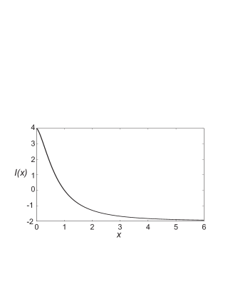
Figure 1: Deformation function $I(x)$.

Using the variation ansatz (7), the exchange energy can be evaluated analytically and is given by

$$E_{ex}=-\frac{\pi d^{2}{\cal V}}{3}\,I(\alpha)\,n_{f}^{2}\,,$$ (8)

where we have defined the “deformation function”:

$$I(x)=\int_{0}^{\pi}d\theta\,\sin\theta\,\left(\frac{3\cos^{2}\theta}{x^{3}\sin^{2}\theta+\cos^{2}\theta}-1\right)\,.$$

This integral has rather complicated analytical form. It is more instructive to plot out the function $I(x)$ which we show in Fig. 1. $I(x)$ is a monotonically decreasing function of $x$, positive for $x<1$, passing through zero at $x=1$ and becomes negative for $x>1$. The exchange energy (8) therefore tends to stretch the Fermi surface along the $z$-axis by taking $\alpha\rightarrow 0$. This however comes with the expense of the kinetic energy

$$E_{kin}=\frac{\cal V}{5}\,\frac{\hbar^{2}k_{F}^{2}}{2m}\,n_{f}\left(\frac{1}{\alpha^{2}}+2\alpha\right)\,,$$

which favors an isotropic spherical Fermi surface (i.e., $\alpha=1$). The competition between the two will find an optimal value of $\alpha$ in the region $\alpha\in(0,\,1)$. The dipolar interaction therefore, through the Fock exchange energy, deforms the Fermi surface of the system. This may be regarded as the magnetostriction effect in momentum space.

Inhomogeneous case — Let us now turn to a system of $N$ atoms confined in a harmonic trapping potential with axial symmetry:

$$U(\bm{r})=\frac{1}{2}m[\omega_{r}^{2}\,(x^{2}+y^{2})+\omega_{z}^{2}\,z^{2}]\,.$$

We choose a variational Wigner function that has the same form as in the homogeneous case, i.e., Eq. (7), but now the Fermi wave number $k_{F}$ is no longer a constant and has the following spatial dependence:

$$k_{F}(\bm{r})=\left\{\tilde{k}_{F}^{2}-\frac{\lambda^{2}}{a_{ho}^{4}}\left[\beta(x^{2}+y^{2})+\frac{1}{\beta^{2}}z^{2}\right]\right\}^{1/2},$$ (9)

where $a_{ho}=\sqrt{\hbar/m\omega}$ and $\omega=(\omega_{r}^{2}\omega_{z})^{1/3}$. The variational parameters $\beta$ and $\lambda$ represent deformation and compression of the dipolar gas in real space, respectively. Using $N=\int d^{3}r\,n(\bm{r})$ one can easily find that $\tilde{k}_{F}=(48N)^{1/6}\lambda^{1/2}/a_{ho}$. The corresponding density distributions in real and momentum space are give by

$$n(\bm{r}) = \frac{\tilde{k}^{3}_{F}}{6\pi^{2}}\left\{1-\frac{1}{R_{F}^{2}}\left[\beta(x^{2}+y^{2})+\frac{1}{\beta^{2}}z^{2}\right]\right\}^{3/2}\,,$$

$$\tilde{n}(\bm{k}) = \frac{R^{3}_{F}}{6\pi^{2}}\left\{1-\frac{1}{\tilde{k}_{F}^{2}}\left[\frac{1}{\alpha}\left({k^{2}_{x}}+k_{y}^{2}\right)-\alpha^{2}{k_{z}^{2}}\right]\right\}^{3/2}\,,$$

respectively, where $R_{F}=(48N)^{1/6}a_{ho}/\lambda^{1/2}$.

Under this ansatz, each term in the energy functional can be evaluated analytically, with the total energy given by, in units of $N^{4/3}\hbar\omega$,

$$\epsilon(\alpha,\beta,\lambda) = c_{1}\left[\lambda\left(2\alpha+\frac{1}{\alpha^{2}}\right)+\frac{1}{\lambda}\left(2\frac{\beta_{0}}{\beta}+\frac{\beta^{2}}{\beta_{0}^{2}}\right)\right]$$ (10)

$$+ c_{2}c_{dd}N^{1/6}\lambda^{3/2}\{I(\beta)-I(\alpha)\}\,,$$

where $c_{1}=3^{1/3}/2^{8/3}\simeq 0.2271$, $c_{2}=2^{10}/(3^{7/2}\cdot 5\cdot 7\pi^{2})\simeq 0.0634$, $c_{dd}=d^{2}/(a_{ho}^{3}\hbar\omega)$, and $\beta_{0}\equiv(\omega_{r}/\omega_{z})^{2/3}$ measures the trap aspect ratio. Here the two terms in the square bracket at rhs represent the kinetic and trapping energy, respectively, while those in the curly bracket are the direct and exchange interaction terms, respectively.

It is not difficult to see that Eq. (10) is not bounded from below, a result arising from the fact that the dipolar interaction is partially attractive. There however exists, under certain conditions, a local minimum in (10), representing a metastable state. This situation is reminiscent of the case of a trapped attractive BEC abec . For the metastable state, the variational energy $\epsilon(\alpha,\beta,\lambda)$ satisfies the Virial theorem $2E_{kin}-2E_{tr}+3(E_{d}+E_{ex})=0$. Hereafter, we refer to the metastable state as the ground state.

We find the ground state by numerically minimizing Eq. (10). Fig. 2 shows the ground state density distributions in both real and momentum space for two different traps. One can see that while the spatial density distributions are essentially determined by the trap geometry, the momentum density distributions by contrast are quite insensitive to the trapping potential and are in both cases elongated along the dipolar direction. Further, the momentum central density at $\bm{k}=0$ decreases as $\beta_{0}$ increases.

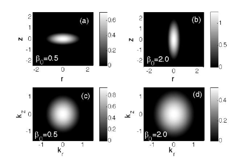
Figure 2: Density distributions in real space (upper plots, in units of $\tilde{k}_{F}^{3}$) and in momentum space (lower plots, in units of $R_{F}^{3}$) for an oblate trap with $\beta_{0}=0.5$ (left plots) and a prolate trap with $\beta_{0}=2$ (right plots). Here $r=\sqrt{x^{2}+y^{2}}$, $k_{r}=\sqrt{k_{x}^{2}+k_{y}^{2}}$ and $c_{dd}N^{1/6}=1.5$.

The stretch in $k_{z}$ is more clearly illustrated in Fig. 3(a), where we have plotted the ratio of the root mean square momentum in $k_{z}$ direction, $\sqrt{\langle k^{2}_{z}\rangle_{0}}$, and to that in $k_{x}$ direction, $\sqrt{\langle k^{2}_{x}\rangle_{0}}$, as a function of the trap aspect ratio $\beta_{0}$ for several dipolar strengths. It turns out that the dipolar interaction leads to nonspherical momentum distribution stretched along the dipolar direction irrespective to the geometry of trapping potential. This can be attributed to the Fock exchange energy that becomes negative for $\alpha<1$ as discussed in the homogeneous system. This result is in stark contrast to the case of dipolar BEC in which the Fock exchange energy is absent and the shape of the momentum distribution is related to that of the spatial distribution through the Fourier transformation. Note that, for non-interacting fermions, the resulting momentum distribution is isotropic independent of the trapping potential Vichi98 ; PSBook .

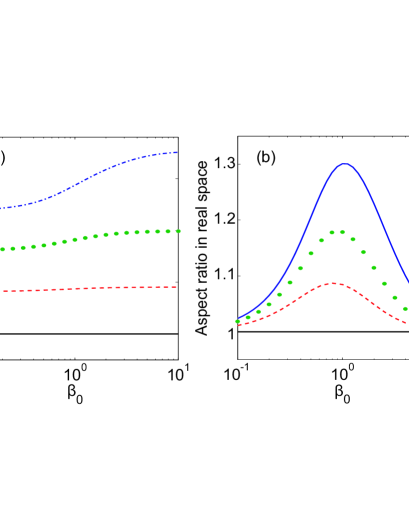
Figure 3: (Color online) (a) Aspect ratio in momentum space $\sqrt{\langle k_{z}^{2}\rangle_{0}/\langle k_{x}^{2}\rangle_{0}}$ and (b) aspect ratio in real space $\sqrt{\langle z^{2}\rangle_{0}/\langle x^{2}\rangle_{0}}$ normalized to that for a non-interacting system as functions of $\beta_{0}$ for $c_{dd}N^{1/6}=0$ (solid line), $0.5$ (dashed line), $1$ (dotted line), and $1.5$ (dot-dashed line).

Figure 4 shows the real space Thomas-Fermi surface of the ground state for different trap geometry. The surface of non-interacting fermions has been plotted as dashed lines for comparison. While the shape of the cloud relies on the trap geometry, the dipolar interaction tends to stretch the gas along the dipolar direction also in real space while compress the gas along the perpendicular radial direction. However, once the trapping potential becomes highly elongated (i.e., $\beta_{0}\gg 1$), the dipolar interaction tends to shrink the whole cloud in both the radial and the axial directions as shown in the case for $\beta_{0}=5$ in Fig. 4. This is because, for such a cigar-shaped trap, a number of dipolar fermions align in the axial (dipolar) direction and feel strong mutual attractions.

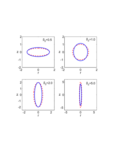
Figure 4: (Color online) Thomas-Fermi surface in real space of the ground state for noninteracting case (dashed line) and for interacting case $c_{dd}N^{1/6}=1.5$ (solid line).

To better quantify the real space deformation, we show in Fig. 3(b) the aspect ratio of the cloud $\sqrt{\langle z^{2}\rangle_{0}/\langle x^{2}\rangle_{0}}$, normalized to that of non-interacting Fermi gas, for different trap geometry. The deviation of the aspect ratio from non-interacting case is most dramatic for near spherical traps with $\beta_{0}\approx 1$.

As we have already pointed out, only metastable dipolar gas can exist in a trap. For sufficiently strong dipolar interaction strengths, Eq. (10) no longer supports the local minimum and the system is expected to be unstable against collapse. For a given trap aspect ratio $\beta_{0}$, the onset of this instability gives rise to a critical value for $c_{dd}N^{1/6}$, yielding the phase diagram as shown in Fig. 5. In Ref. Goral01 , Góral et al. showed that, for a sufficiently oblate trap, the system is always stable regardless of the strength of the dipolar interaction. The critical trap aspect ratio they found is, when translating to our notation, about $\beta_{0}\approx 0.33$. Our calculation, however, indicates that no such critical value exists in $\beta_{0}$ — when the trap becomes more and more oblate, the critical dipolar strength increases rapidly but always remains finite. This contradiction between our work and theirs originates from the Fock exchange term of the dipolar interaction that plays a significant role near critical point and is not properly treated in Ref. Goral01 .

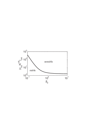
Figure 5: Critical dipolar interaction strength $c_{dd}N^{1/6}$ as a function of $\beta_{0}$.

Finally, let us briefly discuss how to detect the dipolar effects in Fermi gases. In fact, the momentum space magnetostriction effect indicates that the dipolar effects will manifest in time-of-flight images. Assuming ballistic expansion after turning off the trapping potential, for time $t\gg 1/\omega$, the aspect ratio of the expanded cloud approaches the initial in-trap aspect ratio of the momentum distribution as shown in Fig. 3 (a). In other words, regardless of the initial trap geometry, the expanded cloud will eventually become elongated in the dipolar direction. In comparison, the expansion of a non-interacting Fermi gas is isotropic and results in a spherical cloud in the long time limit Vichi98 ; PSBook . The expansion technique has also been used to detect the dipolar effects in chromium BEC. In that case, the expansion dynamics strongly depends on the initial trap geometry Giovanazzi06 ; Lahaye07 .

In conclusion, we have analyzed the properties of a dipolar Fermi gas using a variational method. We have emphasized the important roles played by the Fock exchange energy. We found that the dipolar interaction induces deformation of the Fermi surface and of the phase space density distribution. The resulting anisotropic momentum distribution of the dipolar gas, which can be readily probed using time-of-flight technique, is elongated in dipolar direction irrespective to the trap geometry.

Future work will extend these considerations into collective excitations and superfluidity of the dipolar gas. Since Fermi surface is a key ingredient for low energy properties of Fermi gases, a non-spherical Fermi surface will lead to new features in collective phenomena in dipolar Fermi gases.

This work is supported by the Grant-in-Aid for the 21st Century COE “Center for Diversity and Universality in Physics” from the Ministry of Education, Culture, Sports, Science and Technology (MEXT) of Japan. HP acknowledges support from NSF, the Robert A. Welch Foundation and the W. M. Keck Foundation.

References

- (1) A. Griesmaier et al., Phys. Rev. Lett. 94 160401 (2005).
- (2) C. A. Stan et al., Phys. Rev. Lett. 93, 143001 (2004); S. Inouye et al., Phys. Rev. Lett. 93, 183201 (2004); C. Ospelkaus et al., Phys. Rev. Lett. 97, 120402 (2006); A. J. Kerman et al., Phys. Rev. Lett. 92, 033004 (2004); J. M. Sage et al., Phys. Rev. Lett. 94, 203001 (2005); J. Kleinert et al. Phys. Rev. Lett. 99, 143002 (2007).
- (3) M. Baranov et al., Phys. Scr. T102, 74 (2002).
- (4) S. Ronen, D. C. E. Bortolotti, and J. L. Bohn, Phys. Rev. A 74, 013623 (2006); Phys. Rev. Lett. 98, 030406 (2007).
- (5) K. Góral, L. Santos, and M. Lewenstein, Phys. Rev. Lett. 88, 170406 (2002); S. Yi, T. Li, and C. P. Sun, Phys. Rev. Lett. 98, 260405 (2007).
- (6) S. Yi, L. You, and H. Pu, Phys. Rev. Lett. 93, 040403 (2004); S. Yi, and H. Pu, Phys. Rev. Lett. 97, 020401 (2006); Y. Kawaguchi, H. Saito, and M. Ueda, Phys. Rev. Lett. 97, 130404 (2006).
- (7) K. Góral, B.-G. Englert, and K. Rza̧żewski, Phys. Rev. A 63 033606 (2001).
- (8) K. Góral, M. Brewczyk, and K. Rza̧żewski, Phys. Rev. A 67 025601 (2003).
- (9) O. Dutta, M. Jskelinen, and P. Meystre, Phys. Rev. A 73 043610 (2006).
- (10) M. A. Baranov et al., Phys. Rev. A 66 013606 (2002); M. A. Baranov, . Dobrek, and M. Lewenstein, Phys. Rev. Lett. 92 250403 (2004).
- (11) M. A. Baranov, K. Osterloh, and M. Lewenstein, Phys. Rev. Lett. 94 070404 (2005); K. Osterloh, N. Barberán, and M. Lewenstein, Phys. Rev. Lett. 99 160403 (2007).
- (12) The exchange term is considered in Ref. Goral01 . However, without taking into account the possibility of the deformation of Fermi surface, their treatment of the exchange term is not appropriate.
- (13) M. Köhl et al., Phys. Rev. Lett. 94, 080403 (2005).
- (14) P. Ring and P. Schuck, The Nuclear Many-Body Problem (Springer-Verlag, Berlin, 1980).
- (15) K. Góral and L. Santos, Phys. Rev. A 66, 023613 (2002).
- (16) R. J. Dodd et al., Phys. Rev. A 54, 661 (1996); H. Shi, and W. Zheng, Phys. Rev. A 55, 2930 (1997).
- (17) L. Vichi et al., J. Phys. B 31, L899 (1998).
- (18) L. Pitaevskii and S. Stringari, Bose-Einstein Condensation (Oxford University Press, Oxford, NY, 2003).
- (19) S. Giovanazzi et al., Phys. Rev. A 74, 013621 (2006).
- (20) T. Lahaye et al., Nature (London), 448, 672 (2007).