Multifractal detrended fluctuation analysis of combustion flames in four-burner impinging entrained-flow gasifier

Abstract

On a laboratory-scale testing platform of impinging entrained-flow gasifier with four opposed burners, the flame images for diesel combustion and gasification process were measured with a single charge coupled device (CCD) camera. The two-dimensional multifractal detrended fluctuation analysis was employed to investigate the multifractal nature of the flame images. Sound power-law scaling in the annealed average of detrended fluctuations was unveiled when the order $q>0$ and the multifractal feature of flame images were confirmed. Further analyses identified two multifractal parameters, the minimum and maximum singularity $\alpha_{\min}$ and $\alpha_{\max}$, serving as characteristic parameters of the multifractal flames. These two characteristic multifractal parameters vary with respect to different experimental conditions.

, , , , , ,

1 Introduction

Coal gasification is an important chemical process for coal and the key to realize coal clean utilization. Entrained flow gasification is leading among coal gasification technologies and represents one of the cleanest ways of coal utilization. The entrained-flow gasification technology has been extensively applied to the production of ammonia, methanol, acetic acid, other chemicals and power generation through Integrated Gasification Combined Cycle ($\rm IGCC$). The gasification process of an entrained-flow gasifier is very complicated, because it relates to the fluid flow under the condition of high temperature, high pressure and heterogeneous state. Impinging stream flow configurations are characterized by streams of fluid jets impinging against each other in a confined vessel, which have proved useful in conducting a wide array of chemical engineering unit operations and enhancing heat and mass transfer between phases due to the high transfer coefficients (Tamir, 1994). The opposing jet technique has been applied in many fields and extensively studied both practically (Tamir et al., 1984; Nosseir and Behart, 1986; Berman and Tamir, 1996; Berman et al., 2000a, b; Dehkordi, 2002) and theoretically (Champion and Libby, 1993; Kostiuk and Libby, 1993).

Fractals and multifractals are ubiquitous in natural and social sciences (Mandelbrot, 1983). The fractal behaviour of turbulent premixed flame fronts has been manifested in many experiments (Gouldin, 1987; Gouldin et al., 1989; Murayama and Takeno, 1988; Mantzaras et al., 1989; Goix et al., 1989; Shepherd et al., 1991; North and Santavicca, 1990; Wu et al., 1991; Goix and Shepherd, 1993; Yoshida et al., 1994a, b; Smallwood et al., 1995; Erard et al., 1996; Das and Evans, 1997). These studies provided a quantitative description of flames, which enables us to better understand the dynamics of different types of combustion. On the other hand, to the best of our knowledge, the multifractal nature of impinging flames has not been studied. We shall adopt the two-dimensional multifractal detrended fluctuation analysis (MFDFA) recently developed by Gu and Zhou (2006) for this purpose. The 2D MFDFA is a generalization of the 1D DFA and MFDFA invented by Peng et al. (1994) and Kantelhardt et al. (2002), which is widely used to investigate fractal behavior of time series. The family of DFA approaches have the advantages of easy implementation, high precision, and low computational time (Peng et al., 1994; Kantelhardt et al., 2002; Gu and Zhou, 2006).

The paper is organized as follows. Section 2 reviews the algorithm of the two-dimensional MFDFA in detail. Under each experimental condition, we have recorded many flame images. Rather than analyze the images one by one under the same experimental condition, we propose to perform annealed averaging over dozens of images. The method of annealed averaging is also described. Section 3 outlines the schematic diagram of the experiment setup and the details of the experiments. Section 4 performs multifractal DFA analysis of the flame images, investigates the dependence of multifractal characteristics with respect to experimental conditions, and discusses the physical interpretation of multifractality. Section 5 summarizes.

2 Methodology

2.1 Two-dimensional MFDFA

The idea of DFA was invented originally by Peng et al. (1994) to investigate the long-range dependence in coding and noncoding DNA nucleotide sequences and then generalized by Kantelhardt et al. (2002) to study the multifractal nature hidden in time series, termed as multifractal DFA (MFDFA). Recently, Gu and Zhou (2006) generalized the one-dimensional MFDFA to higher-dimensional version, which is capable of analyzing multifractal properties of higher-dimensional objects. According to Gu and Zhou (2006), the two-dimensional MFDFA consists of the following steps.

Step 1: Consider a flame image $t$, which is denoted by a two-dimensional array $X(t;i,j)$, where $i=1,2,\cdots,M$, $j=1,2,\cdots,N$, and $t=1,2,\cdots,T$. The surface is partitioned into $M_{s}N_{s}$ disjoint square segments of the same size $s\times s$, where $M_{s}=[M/s]$ and $N_{s}=[N/s]$. Each segment can be denoted by $X_{v,w}(t)$ such that $X_{v,w}(t;i,j)=X(t;l_{1}+i,l_{2}+j)$ for $1\leqslant{i,j}\leqslant{s}$, where $l_{1}=(v-1)s$ and $l_{2}=(w-1)s$.

Step 2: For each segment $X_{v,w}(t)$, the cumulative sum $u_{v,w}(t;i,j)$ is calculated as follows:

$$u_{v,w}(t;i,j)=\sum_{k_{1}=1}^{i}\sum_{k_{2}=1}^{j}{X_{v,w}(t;k_{1},k_{2})}~{},$$ (1)

where $1\leqslant{i,j}\leqslant{s}$. Note that $u_{v,w}$ itself is a surface.

Step 3: The trend of the constructed surface $u_{v,w}(t)$ can be determined by fitting it with a prechosen bivariate polynomial function $\widetilde{u}$. In this work, the following polynomial is adopted,

$$\widetilde{u}_{v,w}(t;i,j)=ai^{2}+bj^{2}+cij+di+ej+f~{},$$ (2)

where $1\leqslant{i,j}\leqslant{s}$, and $a$, $b$, $c$, $d$, $e$, and $f$ are free parameters to be determined. These parameters can be estimated easily through simple matrix operations, derived from the least squares method. We can then obtain the residual matrix

$$\epsilon_{v,w}(t;i,j)=u_{v,w}(t;i,j)-\widetilde{u}_{v,w}(t;i,j)~{}.$$ (3)

The detrended fluctuation function $F(t;v,w,s)$ of the segment $X_{v,w}(t)$ is defined via the sample variance of the residual matrix $\epsilon_{v,w}(t;i,j)$ as follows

$$F^{2}(t;v,w,s)=\frac{1}{s^{2}}\sum_{i=1}^{s}\sum_{j=1}^{s}\epsilon_{v,w}(t;i,j)^{2}~{}.$$ (4)

Step 4: The overall detrended fluctuation is calculated by averaging over all the segments, that is,

$$F_{q}(t;s)=\left\{\frac{1}{M_{s}N_{s}}\sum_{v=1}^{M_{s}}\sum_{w=1}^{N_{s}}{[F(t;v,w,s)]^{q}}\right\}^{1/q},$$ (5)

where $q$ can take any real value except for $q=0$. When $q=0$, we have

$$F_{0}(t;s)=\exp\left\{\frac{1}{M_{s}N_{s}}\sum_{v=1}^{M_{s}}\sum_{w=1}^{N_{s}}{\ln[F(t;v,w,s)]}\right\}~{},$$ (6)

according to L’Hôpital’s Rule.

Step 5: Varying the value of $s$ in the range from $s_{\min}\approx 6$ to $s_{\max}\approx\min(M,N)/4$, we can determine the scaling relation between the detrended fluctuation function $F_{q}(t;s)$ and the size scale $s$, which reads

$$F_{q}(t;s)\sim s^{h(q)}~{}.$$ (7)

Usually, the scaling laws hold in a properly determined scaling range.

Since $M$ and $N$ are often not a multiple of the segment size $s$, two orthogonal strips at the end of the profile may remain. In order to take these ending parts of the surface into consideration, the same partitioning procedure can be repeated starting from the other three corners. In this way, we have $4M_{s}N_{s}$ segments and the overall detrended fluctuation is calculated by averaging over them.

The final outcome of the MFDFA analysis is a family of scaling exponents $h(q)$ which is a decreasing function of $q$ for multifractal surface and remains constant for monofractals. In the standard multifractal formalism of Halsey et al. (1986) based on partition functions, the multifractal nature is characterized by the mass exponent ${\tau(q)}$, which is a nonlinear function of $q$ . Kantelhardt et al. (2002) showed that, for each $q$, we can obtain the corresponding traditional ${\tau(q)}$ function through

$$\tau(q)=qh(q)-D_{f}~{},$$ (8)

where $D_{f}$ is the fractal dimension of the geometric support of the multifractal measure. In this work, we have $D_{f}=2$. Resorting to the Legendre transform (Halsey et al., 1986), We can also determine the singularity strength function ${\alpha(q)}$ and the multifractal spectrum $f({\alpha})$ as follows

$$\alpha(q)=h(q)+qh^{\prime}(q)~{},$$ (9)

$$f({\alpha})=q\alpha(q)-\tau(q)~{}.$$ (10)

2.2 Annealed averaging

To achieve better accuracy and higher statistical significance, we perform annealed averaging over 50 images for each experimental condition, which are selected randomly from a huge data base. The annealed averaging gives the means of $F_{q}(s)$ over the selected images,

$$F_{q}(s)=\left\{\frac{1}{T}\sum_{t=1}^{T}[F_{q}(t;s)]^{q}\right\}^{1/q}~{}.$$ (11)

When $q=0$, $F_{0}(s)$ can be calculated according to the following expression

$$\ln[F_{0}(s)]=\frac{1}{T}\sum_{t=1}^{T}\ln[F_{0}(t;s)]~{}.$$ (12)

The characteristic functions of the ensemble of multifractal images can be determined according to Eqs. (7-10).

The shape and width of $f({\alpha})$ curve contain significant information about the singular flame images. In general, the spectrum has a concave downward curvature. We obtain two characteristic quantities, the width of multifractal spectrum $\Delta\alpha=\alpha_{\max}-\alpha_{\min}$ and the difference of fractal dimensions $\Delta f=f(\alpha_{\max})-f(\alpha_{\min})$ of the minimum probability subset with ${\alpha=\alpha_{\max}}$ and the maximum subset with ${\alpha=\alpha_{\min}}$. These two quantities are used in this work to characterize different turbulent flames under different conditions.

3 Experimental equipment and procedure

The schematic drawing of the experimental apparatus is shown in Fig. 1. The maximum values of the operation pressure and temperature were 1 MPa and $1500^{\circ}\mathrm{C}$, respectively. The gasifier was cylindrical, vertically oriented. The combustion chamber was composed of a 15 mm thick cast refractory shell and its inner diameter and length were 300 and 2200 mm, respectively. The cast refractory shell, wrapped with a 235 mm thick and low thermal conductivity fiber blanket to reduce the heat transfer, was protected by a stainless-steel column shell of 0.8 m in diameter and 2.5 m in height. Ports were located on the wall of the gasifier for viewing, temperature measurement, and insertion of a water-cooled probe. Opposed turbulent flow fields were obtained by four opposed round burners composed of inner and outer channels. Oxygen was fed into the outer channels of burners by steel cylinder, with a pressure-reducing valve to avoid pressure oscillations and achieve steady flow. The gas flow rates were measured by mass flow meters (D07-9C/ZM, Beijing Sevenstar Huachuang Electronic Co., Ltd). Diesel oil was fed into the inner channels of burners by a gear pump (A-73004-00 ${\rm\sharp}$, America Cole-Parmer Company), whose flux was determined gravimetrically with an elapsed timer and an electronic weight scale.

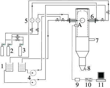
Figure 1: Schematic diagram of experimental apparatus: 1$-$Liquid tank, 2$-$$\rm O_{2}$ steel cylinder, 3$-$$\rm N_{2}$ steel cylinder, 4$-$Pump, 5$-$Gas mass flow meter, 6$-$Burner, 7$-$Vortex flowmeter, 8$-$Slag discharge, 9$-$Flame monitoring system.

In the gasification process, four burners were used to produce opposite jets of fuel that impinge at the center of the combustion chamber. The size of the burners is shown in Fig. 2. High relative velocities between the particulate matter and the gaseous phase in the central area provided good conditions for active diffusion and convection at the particle surface, and the high temperature together resulted in fast burning and gasification reaction under highly reducing conditions to produce raw syngas. High-temperature gaskets interfaced the furnace segments and eliminated all leakage. From the reaction chamber, the raw syngas flowed into the quench chamber, where the raw syngas was cooled and partially scrubbed by water and then discharged. The impinging flames are recorded with a flame monitoring system, fixed on the top of the gasifier. After each experiment, nitrogen was fed into inner channels by a steel cylinder to clean the burners.

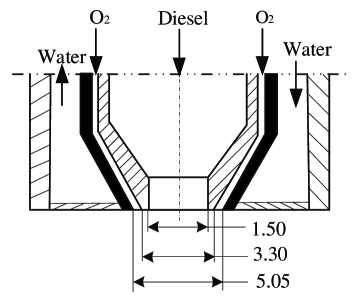
Figure 2: General view of the burner (all dimensions in mm)

The schematic structure of flame image detector is shown in Fig. 3. The flame image detector is fixed on the top refractory wall of the gasifier, and the whole flames are visible during the experimental process. The flame monitoring system consists of a lens, an optical probe, a CCD camera (Panasonic WV-CP470), and a microcomputer. The CCD camera and its accessories are cooled by water to avoid overheating. The objective lens is fixed at the front end of the optical probe and its surface is kept clean against dusts by a jet of nitrogen. The light conveyed by the optical probe enters the CCD camera. The camera has a 1/3-inch high resolution progressive scan interline-transfer CCD sensor with an array of 720 ${\times}$ 576 pixels and each pixel contains 3 bytes (one for each of the fundamental colors: red, green and blue). The video signal is transferred from the CCD camera to the microcomputer and stored.

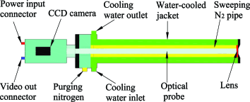
Figure 3: (Color online) Schematic structure of the flame image detector

A typical flame image is illustrated in Fig. 4. The image analysis included the following steps. First, the video signal was digitized into 8-bit (256 gray values for each pixel) two-dimensional digital color images at a rate of 24 frames per second. Second, for each experimental condition, 50 images were analyzed, each of them was converted into grey images with the level ranging from 0 (black) to 255 (white). Third, in order to minimize the possible generated effects of the gasifier wall background, we cropped the grey images to remove most of the gasifier wall background but preserved the whole flame resulting in 200-by-200 images. Four, multifractal analysis was then performed on the 50 resultant images.

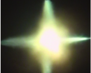
Figure 4: (Color online) The typical four-burner impinging flame image

4 Results and discussion

4.1 Annealed multifractal DFA of images

For each experiment, we performed annealed multifractal DFA on 50 arbitrarily chosen flame images. Fig. 5 shows the dependence of the annealed average of the detrended fluctuations $\ln\left[F_{q}(s)\right]$ with respect to the scale $s$ for six different orders $q$. The nice linearity of the lines indicates power-law scaling between $F_{q}(s)$ and $s$. The scaling range spans about 2.15 orders of magnitude. According to Malcai et al. (1997) and Avnir et al. (1998), the scaling range width for experimental fractality is about 0.5 to 2.0 orders of magnitude. It means that the power-law scaling observed in our experiments are quite sound.

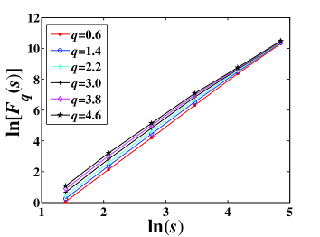
Figure 5: The annealed average of detrended fluctuations $F_{q}(s)$ as a function of the scale $s$ for six different values of $q$

According to Eq. (7), the slopes of the straight lines obtained by least squares regression of $\ln[F_{q}(s)]$ against $\ln(s)$ in Fig. 5 give the estimates of the scaling exponent $h(q)$. In Fig. 6 is illustrated $h(q)$ as a function of $q$ for $0<q\leqslant 5$. We observe that $h(q)$ is a nonlinear function of the order $q$, which is the hallmark of multifractality in the flame images. We note that the estimate of $F_{q}(s)$ becomes statistically less significant for larger $q$ due to the finite size of the flame images. It is also worth stressing that, no evidence of power-law behaviour is observed for $q\leq 0$. In other words, the scale invariance is destroyed for negative $q$. This phenomenon is not unusual in the multifractal analysis of experimental results or natural measures. Examples include the growth probabilities at perimeter sites of diffusion-limited aggregations (DLA) (Lee and Stanley, 1988), the spatial distribution of the secondary electrons on solid surfaces and in the bulk (Li et al., 1995, 1996), the growth probability of a solid-on-solid model (Wang et al., 1995), the TEM images of four-layered GeAl film after laser irradiation (Sanchez et al., 1992), to list a few.

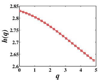
Figure 6: Dependence of $h(q)$ with respect to $q$

The values of $\alpha(q)$ and $f(\alpha)$ can be computed numerically based on the Legendre transform (9,10). The resulting multifractal curve $f(\alpha)$ is plotted in Fig. 7 with respect to $\alpha$. Two fundamental quantities $\alpha_{\min}$ and $\alpha_{\max}$ are determined, which characterize respectively the minimal and maximal singular sites of the turbulent flames. Moreover, the width of singularity strength $\Delta\alpha=\alpha_{\max}-\alpha_{\min}$ can be used as a measure of heterogeneity of the singular flames. Similarly, $f(\alpha_{\min})$, $f(\alpha_{\max})$, and $\Delta{f}=f(\alpha_{\max})-f(\alpha_{\min})$ can also be used to quantitatively characterize the multifractal nature of the flames.

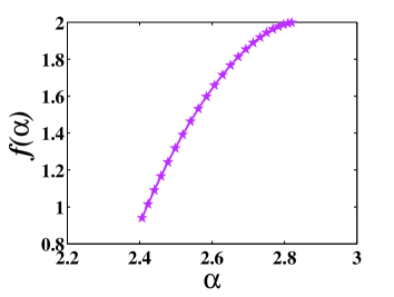
Figure 7: Multifractal spectrum for the flame images

4.2 Relationship between multifractal parameters and experimental conditions

In our experiments, we have investigated 95 conditions by varying the burner exit velocities of diesel and oxygen, $M({\rm{m}}/{\rm{s}})$ and $V({\rm{m}}^{3}/{\rm{s}})$. Under each experimental condition, 50 flame images have been used to calculate the ensemble multifractal parameters $\alpha_{\min}$, $\alpha_{\max}$, $\Delta\alpha$, $f(\alpha_{\min})$, $f(\alpha_{\max})$, and $\Delta{f}$. Here we investigate the possible dependence of these multifractal parameters with respect to experimental parameters $M$ and $V$ to identify characteristic multifractal parameters. Specifically, we adopt linear models as follows

$${\rm{MF}}=\beta_{0}+\beta_{1}M+\beta_{2}V~{},$$ (13)

where ${\rm{MF}}$ stands for the six individual multifractal parameters. We investigate three different types of models by posing $\beta_{1}=0$ or $\beta_{2}=0$ or freeing $\beta_{1}$ and $\beta_{2}$. This gives 18 models in total. For each model, we use the F-test to check if the model is statistically significant. If the model is significant, we employ further the t-test to see whether the model coefficients are significantly different from zero or not.

As a first step, we consider the six monovariate models with $\beta_{1}=0$. The F-tests show that the four models for $\Delta\alpha$, $f(\alpha_{\min})$, $f(\alpha_{\max})$ and $\Delta{f}$ are not significant, where all the $p$-values are greater than 13%. On the other hand, the $p$-values for $\alpha_{\min}$ and $\alpha_{\max}$ are both 0.1%. This implies that both the multifractal parameters $\alpha_{\min}$ and $\alpha_{\max}$ are linearly dependent on the burner exit velocity $V$ of oxygen. In addition, according to the t-tests, we find that the $p$-values of $\beta_{0}$ and $\beta_{2}$ in these two models are not greater than 0.1%. In other words, the coefficients $\beta_{0}$ and $\beta_{2}$ are significantly different from zero.

Then, we investigate the six monovariate models with $\beta_{2}=0$. The F-tests show that the five models for $\alpha_{\min}$, $\Delta\alpha$, $f(\alpha_{\min})$, $f(\alpha_{\max})$ and $\Delta{f}$ are not significant, where all the $p$-values are greater than 29%, while the $p$-values for $\alpha_{\max}$ is 4.5%. This means that the multifractal parameter $\alpha_{\max}$ is linearly dependent on the burner exit velocity $M$ of diesel, significant at the 5% level. In addition, according to the t-test, we find that the $p$-values of $\beta_{0}$ and $\beta_{1}$ in this model are not greater than 5%. In other words, the coefficients $\beta_{0}$ and $\beta_{1}$ are significantly different from zero.

Now we turn to study the six bivariate models (13) with different dependent variables ${\rm{MF}}$. The resluts are listed in Table 1. According to the F-tests, the four models for $\Delta\alpha$, $f(\alpha_{\min})$, $f(\alpha_{\max})$ and $\Delta{f}$ are not significant whose $p$-values are greater than 14%. For $\alpha_{\min}$ and $\alpha_{\max}$, the $p$-values obtained from the F-tests are less than 1%. Therefore, both the multifractal parameters $\alpha_{\min}$ and $\alpha_{\max}$ are linearly dependent on the velocities of oxygen and diesel. However, the t-tests shows that the coefficients $\beta_{1}$ for both models are not significantly different from zero. Speaking differently, the multifractal parameters $\alpha_{\min}$ and $\alpha_{\max}$ depend strong upon the burner exit velocity of oxygen and weakly on the velocity of diesel. Furthermore, the minimal and maximal singularity strengthes $\alpha_{\min}$ and $\alpha_{\max}$ are characteristic multifractal parameters that can be used to quantify the multifractal nature of the turbulence flames.

Table 1: Identification of characteristic multifractal parameters using linear model (13)

	Coefficients				t-test				F-test
${\rm{MF}}$	$\beta_{0}$	$\beta_{1}$	$\beta_{2}$		$p_{0}$	$p_{1}$	$p_{2}$		$F$	$p$
$\alpha_{\min}$	2.4734	0.4538	-0.0027		0.000	0.589	0.001		5.576	0.005
$\alpha_{\max}$	3.1728	-0.6503	-0.0013		0.000	0.117	0.002		7.477	0.001
$f(\alpha_{\min})$	0.3067	2.1950	-0.0011		0.649	0.260	0.555		0.729	0.485
$f(\alpha_{\max})$	1.9911	-0.0576	0.0002		0.000	0.610	0.118		1.279	0.283
$\Delta\alpha$	0.6992	-1.1035	0.0014		0.023	0.208	0.094		1.942	0.149
$\Delta f$	1.6845	-2.2529	0.0013		0.013	0.243	0.491		0.822	0.443

4.3 Discussion

We have confirmed that the impinging flame images exhibit multifractal properties. A natural question arises asking which processes lead to such multifractality. Several examples taken from other fields in literature provide clues for addressing this question. Godano et al. (1997) argued that the multifractal nature of the temporal clustering of earthquakes can be interpreted in terms of diffusive processes of stress in the Earth’s crust. In order to explain the multifractal properties in rainfall data, Olsson and Niemczynowicz (1996) made an assumption that a large-scale flux is successively broken into smaller and smaller ones in cascades, each receiving an amount of the total flux specified by a multiplicative process. Lee (2002) and Lee et al. (2003) also employed a random multiplicative process to understand the multifractal characteristics in air pollutant concentration time series. In the present case, we submit that a possible explanation for the physical origin of multifractality in flame images is the atomization and impinging processes.

Due to the complexity of the atomization process, it is difficult to clearly describe the mechanism and also impossible to combine all the influencing factors into one model, such as the equipment dimensions, the size and geometry of burner, the physical properties of the dispersed phase and the continuous phase, and the operating mode. Indeed, Zhou et al. (2000) proposed a stochastic multiplicative cascade model for drop breakdown in atomization processes, which works well in the prediction of drop size distribution (Liu et al., 2006). Moreover, Zhou and Yu (2001) studied the multifractal nature of drop breakup in the air-blast burner atomization process. They applied the multiplier method to extract the negative and the positive parts of the $f(\alpha)$ curve with the data of drop-size distribution measured using dual particle dynamic analyzer. They proposed a random multifractal model with the multiplier triangularly distributed to characterize the breakup of drops, the agreement of the left part ($q>0$) of the multifractal spectrum between the experimental result and the model is remarkable. Hence, the breakdown of diesel drops in the gasifier follows a multifractal process.

Four equal suspension streams flow against one another at high velocity ($>35~{}$m/s) and impinge at the center of the gasifier, resulting in a highly turbulent zone. The gas flows decrease their axial velocity down to zero at the impingement plane and then disperse radially, while particles penetrate back and forth between the opposed streams driven by inertia and friction forces. This impinging process leads to locally singular distributions of the raw materials.

5 Conclusion

The impinging process has proved to be one of the most effective methods enhancing heat and mass transfer in multiphase environment. On a laboratory-scale testing platform of impinging entrained-flow gasifier with four opposed burners, the flame images for diesel combustion and gasification process were measured with a single charge coupled device (CCD) camera. Ninety-five experimental conditions were investigated.

The multifractal properties of the turbulent flames have been investigated using the two-dimensional multifractal detrended fluctuation analysis, which is accurate and easy to implement for image analysis. Nice power-law scaling is unveiled in the annealed average of detrended fluctuations when the order $q>0$. The scaling exponent $h(q)$ is a nonlinear function of $q$, which confirms the multifractal nature of the flames under investigation. We argue that the multifractality in gasification flames stems from the multiplicative process of atomization and the impinging process of raw materials.

We analyzed the relationship between six multifractal parameters ($\alpha_{\min}$, $\alpha_{\max}$, $\Delta\alpha$, $f(\alpha_{\min})$, $f(\alpha_{\max})$ and $\Delta{f}$) and the velocities of oxygen and diesel ($V$ and $M$). Two multifractal parameters $\alpha_{\min}$ and $\alpha_{\max}$ have been identified by extensive F-tests as characteristics of the observed multifractal nature, which are dependent on the velocities linearly. The t-tests show that the velocity of oxygen has greater impact on the multifractality of flames. These analyses enable us to gain a better understanding of the complexity of the combustion dynamics of four-burner impinging entrained-flow gasification.

Acknowledgments:

We are grateful to Gao-Feng Gu for useful discussions. This work was partially supported by the National Basic Research Program of China (No. 2004CB217703), the PCSIRT (IRT0620), the Program for New Century Excellent Talents in University (NCET-05-0413), and the Project Sponsored by the Scientific Research Foundation for the Returned Overseas Chinese Scholars, State Education Ministry.

References

- Avnir et al. (1998) Avnir, D., Biham, O., Lidar, D., Malcai, O., 1998. Is the geometry of nature fractal? Science 279, 39–40.
- Berman and Tamir (1996) Berman, Y., Tamir, A., 1996. Experimental investigation of phosphate dust collection in impinging streams (IS). Canadian Journal of Chemical Engineering 74, 817–821.
- Berman et al. (2000a) Berman, Y., Tanklevsky, A., Oren, Y., Tamir, A., 2000a. Modeling and experimental studies of absorption in coaxial cylinders with impinging streams: Part I. Chemical Engineering Science 55, 1009–1021.
- Berman et al. (2000b) Berman, Y., Tanklevsky, A., Oren, Y., Tamir, A., 2000b. Modeling and experimental studies of absorption in coaxial cylinders with impinging streams: part II. Chemical Engineering Science 55, 1023–1028.
- Champion and Libby (1993) Champion, M., Libby, P. A., 1993. Reynolds stress description of opposed and impinging turbulent jets. Part I: Closely spaced opposed jets. Physics of Fluids A 5, 203–216.
- Das and Evans (1997) Das, A. K., Evans, R. L., 1997. An experimental study to determine fractal parameters for lean premixed flames. Experiments in Fluids 22, 312–320.
- Dehkordi (2002) Dehkordi, A. M., 2002. Application of a novel-opposed-jets contacting device in liquid-liquid extraction. Chemical Engineering & Processing 41, 251–258.
- Erard et al. (1996) Erard, V., Boukhalfa, A., Puechberty, D., Trinité, M., 1996. A statistical study on surface properties of freely-propagating premixed turbulent flames. Combustion Science and Technology 113-114, 313–327.
- Godano et al. (1997) Godano, C., Alonzo, M. L., Vilardo, G., 1997. Multifractal approach to time clustering of earthquakes application to Mt. Vesuvio seismicity. Pure and Applied Geophysics 149, 375–390.
- Goix and Shepherd (1993) Goix, P., Shepherd, I. G., 1993. Lewis number effects on turbulent premixed flame structure. Combustion Science and Technology 91, 191–206.
- Goix et al. (1989) Goix, P. J., Shepherd, I. G., Trinité, M., 1989. A fractal study of a premixed V-shaped /air flame. Combustion Science and Technology 63, 275–286.
- Gouldin (1987) Gouldin, F. C., 1987. An application of fractals to modeling premixed turbulent flames. Combustion and Flame 68, 249–266.
- Gouldin et al. (1989) Gouldin, F. C., Hilton, S. M., Lamb, T., 1989. Experimental evaluation of the fractal geometry of flamelets. Symposium (International) on Combustion 22, 541–550.
- Gu and Zhou (2006) Gu, G.-F., Zhou, W.-X., 2006. Detrended fluctuation analysis for fractals and multifractals in higher dimensions. Physical Review E 74, 061104.
- Halsey et al. (1986) Halsey, T. C., Jensen, M. H., Kadanoff, L. P., Procaccia, I., Shraiman, B. I., 1986. Fractal measures and their singularities: The characterization of strange sets. Physical Review A 33, 1141–1151.
- Kantelhardt et al. (2002) Kantelhardt, J. W., Zschiegner, S. A., Koscielny-Bunde, E., Havlin, S., Bunde, A., Stanley, H. E., 2002. Multifractal detrended fluctuation analysis of nonstationary time series. Physica A 316, 87–114.
- Kostiuk and Libby (1993) Kostiuk, L. W., Libby, P. A., 1993. Comparison between theory and experiment for turbulence in opposed streams. Physics of Fluids A 5, 2301–2303.
- Lee (2002) Lee, C. K., 2002. Multifractal characteristics in air pollutant concentration time series. Water, Air, and Soil Pollution 135, 389–409.
- Lee et al. (2003) Lee, C. K., Ho, D. S., Yu, C. C., Wang, C. C., Hsiao, Y. H., 2003. Simple multifractal cascade model for the air pollutant concentration time series. Environmetrics 14, 255–269.
- Lee and Stanley (1988) Lee, J., Stanley, H. E., 1988. Phase transition in the multifractal spectrum of diffusion-limited aggregation. Physical Review Letters 61, 2945–2948.
- Li et al. (1995) Li, H., Ding, Z.-J., Wu, Z.-Q., 1995. Multifractal behavior of the distribution of secondary emission sites on solid surfaces. Physical Review B 51, 13554–13559.
- Li et al. (1996) Li, H., Ding, Z.-J., Wu, Z.-Q., 1996. Multifractal analysis of the spatial distribution of secondary-electron emission sites. Physical Review B 53, 16631–16636.
- Liu et al. (2006) Liu, H.-F., Gong, X., Li, W.-F., Wang, F.-C., Yu, Z.-H., 2006. Prediction of droplet size distribution in sprays of prefilming air-blast atomizers. Chemical Engineering Science 61, 1741–1747.
- Malcai et al. (1997) Malcai, O., Lidar, D. A., Biham, O., Avnir, D., 1997. Scaling range and cutoffs in empirical fractals. Physical Review E 56, 2817–2828.
- Mandelbrot (1983) Mandelbrot, B. B., 1983. The Fractal Geometry of Nature. W. H. Freeman, New York.
- Mantzaras et al. (1989) Mantzaras, J., Felton, P. G., Bracco, F. V., 1989. Fractals and turbulent premixed engine flames. Combustion and Flame 77, 295–310.
- Murayama and Takeno (1988) Murayama, M., Takeno, T., 1988. Fractal-like character of flamelets in turbulent premixed combustion. Symposium (International) on Combustion 22, 551–559.
- North and Santavicca (1990) North, G. L., Santavicca, D. A., 1990. The fractal nature of premixed turbulent flames. Combustion Science and Technology 72, 215–232.
- Nosseir and Behart (1986) Nosseir, N. S., Behart, S., 1986. Characteristics of jet impingement in a side-dump combustor. AIAA Journal 24, 1752–1757.
- Olsson and Niemczynowicz (1996) Olsson, J., Niemczynowicz, J., 1996. Multifractal analysis of daily spatial rainfall distributions. Journal of Hydrology 187, 29–43.
- Peng et al. (1994) Peng, C.-K., Buldyrev, S. V., Havlin, S., Simons, M., Stanley, H. E., Goldberger, A. L., 1994. Mosaic organization of DNA nucleotides. Physical Review E 49, 1685–1689.
- Sanchez et al. (1992) Sanchez, A., Serna, R., Catalina, F., Afonso, C., 1992. Multifractal patterns formed by laser irradiation in GeAl thin multilayer films. Physical Review B 46, 487–490.
- Shepherd et al. (1991) Shepherd, I. G., Cheng, R. K., Goix, P. J., 1991. The spatial scalar structure of premixed turbulent stagnation point flames. Symposium (International) on Combustion 23, 781–787.
- Smallwood et al. (1995) Smallwood, G. J., Gülder, Ö. L., Snelling, D. R., Deschamps, B. M., Gökalp, I., 1995. Characterization of flame front surfaces in turbulent premixed methane/air combustion. Combustion and Flame 101, 461–470.
- Tamir (1994) Tamir, A., 1994. Impinging-Stream Reactors: Fundamentals and Applications. Elsevier, Amsterdam.
- Tamir et al. (1984) Tamir, A., Elperin, I., Luzzatto, K., 1984. Drying in a new two impinging streams reactor. Chemical Engineering Science 39, 139–146.
- Wang et al. (1995) Wang, B., Wang, Y., Wu, Z.-Q., 1995. Multifractal behavior of solid-on-solid growth. Solid State Communications 96, 69–72.
- Wu et al. (1991) Wu, M. S., Kwon, S., Driscoll, J. F., Faeth, G. M., 1991. Preferential diffusion effects on the surface stucture of turbulent premixed hydrogen/air flames. Combustion Science and Technology 78, 69–96.
- Yoshida et al. (1994a) Yoshida, A., Ando, Y., Yanagisawa, T., Tsuji, H., 1994a. Fractal behavior of wrinkled laminar flame. Combustion Science and Technology 96, 121–134.
- Yoshida et al. (1994b) Yoshida, A., Kasahara, M. Tsuji, H., Yanagisawa, T., 1994b. Fractal geometry application in estimation of turbulent burning velocity of wrinkled laminar flame. Combustion Science and Technology 103, 207–218.
- Zhou and Yu (2001) Zhou, W.-X., Yu, Z.-H., 2001. Multifractality of drop breakup in the air-blast nozzle atomization process. Physical Review E 63, 016302.
- Zhou et al. (2000) Zhou, W.-X., Zhao, T.-J., Wu, T., Yu, Z.-H., 2000. Application of fractal geometry to atomization process. Chemical Engineering Journal 78, 193–197.