Constraints on dark matter particles from theory, galaxy observations and N-body simulations.
Abstract
Mass bounds on dark matter (DM) candidates are obtained for particles that decouple in or out of equilibrium while ultrarelativistic with arbitrary isotropic and homogeneous distribution functions. A coarse grained Liouville invariant primordial phase space density is introduced which depends solely on the distribution function at decoupling. The density is explicitly computed and combined with recent photometric and kinematic data on dwarf spheroidal satellite galaxies in the Milky Way (dShps) and the observed DM density today yielding upper and lower bounds on the mass, primordial phase space densities and velocity dispersion of the DM candidates. Combining these constraints with recent results from -body simulations yield estimates for the mass of the DM particles in the range of a few keV. We establish in this way a direct connection between the microphysics of decoupling in or out of equilibrium and the constraints that the particles must fulfill to be suitable DM candidates. If chemical freeze out occurs before thermal decoupling, light bosonic particles can Bose-condense. We study such Bose-Einstein condensate (BEC) as a dark matter candidate. It is shown that depending on the relation between the critical () and decoupling () temperatures, a BEC light relic could act as CDM but the decoupling scale must be higher than the electroweak scale. The condensate hastens the onset of the non-relativistic regime and tightens the upper bound on the particle’s mass. A non-equilibrium scenario which describes particle production and partial thermalization, sterile neutrinos produced out of equilibrium and other DM models is analyzed in detail and the respective bounds on mass, primordial phase space density and velocity dispersion are obtained. Thermal relics with that decouple when ultrarelativistic and sterile neutrinos produced resonantly or non-resonantly lead to a primordial phase space density compatible with cored dShps and disfavor cusped satellites. Light Bose-condensed DM candidates yield phase space densities consistent with cores and if also with cusps. Phase space density bounds on particles that decoupled non-relativistically combined with recent results from N-body simulations suggest a potential tension for WIMPs with .
pacs:
98.80.Cq,05.10.Cc,11.10.-zI Introduction
Although the existence of dark matter (DM) was inferred several decades ago zwoo , its nature still remains elusive. Candidate dark matter particles are broadly characterized as cold, hot or warm depending on their velocity dispersions. The clustering properties of collisionless DM candidates in the linear regime depend on the free streaming length, which roughly corresponds to the Jeans length with the particle’s velocity dispersion replacing the speed of sound in the gas. Cold DM (CDM) candidates feature a small free streaming length favoring a bottom-up hierarchical approach to structure formation, smaller structures form first and mergers lead to clustering on the larger scales.
Among the CDM candidates are weakly interacting massive particles (WIMPs) with . Hot DM (HDM) candidates feature large free streaming lengths and favor top down structure formation, where larger structures form first and fragment. HDM particle candidates are deemed to have masses in the few range, and warm DM (WDM) candidates are intermediate with a typical mass range .
The concordance standard cosmological
model emerging from CMB, large scale structure observations and
simulations favors the hypothesis that DM is composed of primordial
particles which are cold and collisionless primack . However,
recent observations hint at possible discrepancies with the
predictions of the concordance model: the
satellite and cuspy halo problems.
The satellite problem, stems from
the fact that CDM favors the presence of substructure: much of the
CDM is not smoothly distributed but is concentrated in small lumps,
in particular in dwarf galaxies for which there is scant observational
evidence so far. A low number of satellites have been observed in
Milky-Way sized galaxies kauff ; moore ; moore2 ; klyp . This substructure is a
consequence of the CDM power spectrum which favors small scales
becoming non-linear first, collapsing in the bottom-up
hierarchical manner and surviving the mergers as dense clumps
moore ; klyp .
The cuspy halo problem arises from the result of large scale
-body simulations of CDM clustering which predict a monotonic
increase of the density towards the center of the halos
dubi ; frenk ; moore2 ; bullock ; cusps , for example the universal
Navarro-Frenk-White (NFW) profile frenk which describes accurately clusters of galaxies, but
indicates a divergent cusp at the center of the halo. Recent
observations seem to indicate central cores in dwarf
galaxies dalcanton1 ; van ; swat ; gilmore , leading to the ’cusps
vs cores’ controversy.
A recent compilation of observations of dwarf spheroidal galaxies dSphs gilmore , which are considered to be prime candidates for DM subtructure spergel , seem to favor a core with a smoother central density and a low mean mass density rather than a cusp gilmore . The data cannot yet rule out cuspy density profiles which allow a maximum density and the interpretation and analysis of the observations is not yet conclusive dalcanton1 ; van2 . These possible discrepancies have rekindled an interest in WDM particles, which feature a velocity dispersion larger than CDM particles, and consequently larger free-streaming lengths which smooth-out the inner cores and would be prime candidates to relieve the cuspy halo and satellite problems turok .
A possible WDM candidate is a sterile neutrino dw ; este ; kusenko with a mass in the range and produced via their mixing and oscillation with an active neutrino species either non-resonantly dw , or through MSW (Mikheiev-Smirnov-Wolfenstein) resonances in the medium este . Sterile neutrinos can decay into a photon and an active neutrino (more precisely the largest mass eigenstate decays into the lowest one and a photon) pal yielding the possibility of direct constraints on the mass and mixing angle from the diffuse X-ray background Xray .
Observations of cosmological structure formation via the Lyman- forest provide a complementary probe of primordial density fluctuations on small scales which yield an indirect constraint on the masses of WDM candidates. While constraints from the diffuse X-ray background yield an upper bound on the mass of a putative sterile neutrino in the range Xray , the latest Lyman- analysis lyman yields lower bounds in the range in tension with the X-ray constraints. More recent constraints from Lyman- yield a lower limit for the mass of a WDM candidate for an early decoupled thermal relic and for sterile neutrinos viel . Strong upper limits on the mass and mixing angles of sterile neutrinos have been recently discussed beacom , however, there are uncertainties as to whether WDM candidates can explain large cores in dSphs strigari . It has been recently argued palazzo that if sterile neutrinos are produced non-resonantly dw the combined X-ray and Lyman- data suggest that these cannot be the only WDM component, with an upper limit for their fractional relic abundance . Recent boyarski2 constraints on a radiatively decaying DM particle from the EPIC spectra of (M31) by XMM-Newton confirms this result and places a stronger lower mass limit .
All these results suggest that DM could be a mixture of several components with sterile neutrinos as viable candidates.
Motivation and goals: Although the paradigm describes large scale structure formation remarkably well, the possible small scale discrepancies mentioned above motivate us to study new constraints that different dark matter components must fulfill to be suitable candidates. Cosmological bounds on dark matter components primarily focused on standard model neutrinos bond ; TG , heavy relics that decoupled in local thermodynamic equilibrium (LTE) when non-relativistic LW ; kt ; dominik or thermal ultrarelativistic relics madsen ; madsenbec ; madsenQ ; salu ; hogan . More recently, cosmological precision data were used to constrain the (HDM) abundance of low mass particles pastor ; steen ; raffelt ; mena assuming these to be thermal relics.
The main results of this article are:
(a:) We consider particles that decouple in or out of LTE during the radiation dominated era with an arbitrary (but homogeneous and isotropic) distribution function. Particles which decouple being ultrarelativistic eventually become non-relativistic because of redshift of physical momentum. We establish a direct connection between the microphysics of decoupling in or out of LTE and the constraints that the particles must fulfill to be suitable DM candidates in terms of the distribution functions at decoupling.
(b:) We introduce a primordial coarse grained phase space density
where is the number of particles per unit physical volume and is the average of the physical momentum with the distribution function of the decoupled particle. is a Liouville invariant after decoupling and only depends on the distribution functions at decoupling. In the non-relativistic regime is simply related to the phase densities considered in refs. dalcanton1 ; TG ; hogan ; madsenQ and can only decrease by collisionless phase mixing or self-gravity dynamics theo .
In the non-relativistic regime we obtain
| (1) |
where is the primordial one-dimensional velocity dispersion and the dark matter density. Combining the result for the primordial phase space density determined by the mass and the distribution function of the decoupled particles, with the recent compilation of photometric and kinematic data on dSphs satellites in the Milky-Way gilmore yields lower bounds on the DM particle mass whereas upper bounds on the DM mass are obtained using the value of the observed dark matter density today. Therefore the combined analysis of observational data from (dSphs), N-body simulations and the present DM density allows us to establish both upper and lower bounds on the mass of the DM candidates.
We thus provide a link between the microphysics of decoupling, the observational aspects of dark matter halos and the DM mass value.
(c:) Recent -body simulations numQ indicate that the phase-space density decreases a factor during gravitational clustering. This result combined with eq.(1) and the observed values on dSphs satellites gilmore yield
for the masses of thermal relics DM candidates, where ‘cored’ and ’cusp’ refer to the type of profile used in the dShps description and is the number of internal degrees of freedom of the DM particle. Wimps with masses decoupling in LTE at temperatures lead to primordial phase space densities many orders of magnitude larger than those observed in (dSphs). The results of -body simulations, which yield relaxation by orders of magnitudenumQ suggest a potential tension for WIMPs as DM candidates. However, the -body simulations in ref.numQ begin with initial conditions with values of the phase space density much lower than the primordial one. Hence it becomes an important question whether the enormous relaxation required from the primordial values to those of observed in dSphs can be inferred from numerical studies with suitable (much larger) initial values of the phase space density.
(d:) We study the possibility that the DM particle is a light Boson that undergoes Bose-Einstein Condensation (BEC) prior to decoupling while still ultrarelativistic. (This possibility was addressed in madsenbec ). We analyze in detail the constraints on such BEC DM candidate from velocity dispersion and phase space arguments, and contrast the BEC DM properties to those of the hot or warm thermal relics.
(e:) Non-equilibrium scenarios that describe various possible WDM candidates are studied in detail. These scenarios describe particle production boydata and incomplete thermalization dvd , resonant dw and non-resonant este production of sterile neutrinos and a model recently proposed strigari to describe cores in dSphs.
Our analysis of the DM candidates is based on their masses, statistics and properties at decoupling (being it in LTE or not). We combine observations on dSphs gilmore and -body simulations numQ , with theoretical analysis using the non-increasing property of the phase space density TG ; dalcanton1 ; hogan ; theo .
The results from the combined analysis of the primordial phase space densities, the observational data on dSphs gilmore and the -body simulations in ref.numQ are the following:
-
•
(i): conventional thermal relics, and sterile neutrinos produced resonantly or non-resonantly with mass in the range that decouple when ultrarelativistic lead to a primordial phase space density of the same order of magnitude as in cored dShps and disfavor cusped satellites for which the data gilmore yields a much larger phase space density.
-
•
(ii): CDM from wimps that decouple when non-relativistic with and kinetic decoupling at dominik yield phase space densities at least eighteen to fifteen orders of magnitude [see eqs.(121), (122) and (128)] larger than the typical average in dSphs gilmore . Results from -body simulations, albeit with initial conditions with much smaller values of the phase space density, yield a dynamical relaxation by a factor numQ . If these results are confirmed by simulations with larger initial values there may be a potential tension between the primordial phase space density for thermal relics in the form of WIMPs with MeV and those observed in dShps.
-
•
(iii): Light bosonic particles decoupled while ultrarelativistic and which form a BEC lead to phase space densities consistent with cores and also consistent with cusps if . However if these thermal relics satisfy the observational bounds, they must decouple when , namely above the electroweak scale.
Section II analyzes the generic dynamics of decoupled particles for any distribution function, with or without LTE at decoupling, and for different species of particles. In section III we consider light thermal relics which decoupled in LTE as DM components: fermions and bosons, including the possibility of a Bose-Einstein condensate. Section IV deals with coarse grained phase space densities which are Liouville invariant and the new bounds obtained with them by using the observational dSphs data and recent results from -body simulations, bounds from velocity dispersion, and the generalized Gunn-Tremaine bound. In Section V we study the case of particles that decoupled out of equilibrium and the consequences on the dark matter constraints. Section VI summarizes our conclusions.
II Preliminaries: dynamics of decoupled particles
While the study of kinetics in the early Universe is available in the literature bernstein ; kt ; scott , in this section we expand on the dynamics of decoupled particles emphasizing several aspects relevant to the analysis that follows in the next sections.
Consider a spatially flat FRW cosmology with length element
| (2) |
the non-vanishing Christoffel symbols are
| (3) |
The (contravariant) four momentum is defined as with an affine parameter, so that , where is the mass of the particle. This leads to the dispersion relation
| (4) |
The geodesic equations are
| (5) | |||
| (6) | |||
| (7) |
where and we used . The solution of eq.(7) is
| (8) |
where is the time independent comoving momentum. The local observables, energy and momentum as measured by an observer at rest in the expanding cosmology are given by
| (9) |
where form a local orthonormal tetrad (vierbein)
and the sign in eq.(9) corresponds to a space-like component. For the FRW metric
| (10) |
and we find,
| (11) |
is clearly the physical momentum, redshifting with the expansion. Combining the above with eq.(4) yields the local dispersion relation
| (12) |
A frozen distribution describing a particle that has been decoupled from the plasma is constant along geodesics, therefore, taking the distribution to be a function of the physical momentum and time, it obeys the Liouville equation or collisionless Boltzmann equation
| (13) |
Taking as an independent variable this equation leads to the familiar form
| (14) |
Obviously a solution of this equation is
| (15) |
where is the time independent comoving momentum. The physical phase space volume element is invariant, , where refer to physical and comoving volumes respectively.
The scale factor is normalized so that
| (16) |
and , where is the cosmic time at decoupling and is the redshift.
If a particle of mass has been in LTE but it decoupled from the plasma with decoupling temperature its distribution function is
| (17) |
for fermions or bosons respectively allowing for a chemical potential at decoupling.
In what follows we consider general distributions as in eq.(15) unless specifically stated.
The kinetic energy momentum tensor associated with this frozen distribution is given by
| (18) |
where is the number of internal degrees of freedom, typically . Taking the distribution function to be isotropic it follows that
| (19) | |||
| (20) |
where is the energy density and is the pressure. In summary,
| (21) |
The pressure can be written in a manner more familiar from kinetic theory as
| (22) |
where is the physical (group) velocity of the particles measured by an observer at rest in the expanding cosmology.
To confirm covariant energy conservation recall that , furthermore from eq.(5) it follows that , leading to
| (23) |
the first term results from the measure and the last term from ; from the expression of the pressure eq.(20) the covariant conservation equation
| (24) |
follows. The number of particles per unit physical volume is
| (25) |
and obeys
| (26) |
namely, the number of particles per unit comoving volume is conserved.
These are generic results for the kinetic energy momentum tensor and the particle density for any distribution function that obeys the collisionless Boltzmann equation (13).
The entropy density for an arbitrary distribution function for particles that decoupled in or out of LTE is
| (27) |
where the upper and lower signs refer to Fermions and Bosons respectively. Since it follows that
| (28) |
therefore the entropy per comoving volume is constant. In particular the ratio
| (29) |
is a constant for any distribution function that obeys the collisionless Liouville equation kt .
In the case of LTE, using the distribution eq.(17) in the entropy density eq.(27) yields the result
| (30) |
for either statistics, where are evaluated at the decoupling time . The entropy of the gas of decoupled particles does not affect the relationship between the photon temperature and the temperature of ultrarelativistic particles that decouple later which can be seen as follows.
Consider several species of particles, one of which decouples at an earlier time in or out of equilibrium with the distribution function and entropy given by eq.(27) while the others remain in LTE with entropy density , until some of them decouple later while ultrarelativistic. Here is the temperature at time and is the effective number of ultrarelativistic degrees of freedom. Entropy conservation leads to the relation,
| (31) |
however, because , the usual relation , relating the temperature of a gas of ultrarelativistic decoupled particles to the photon temperature follows.
For light particles that decouple in LTE at temperature we can approximate
| (32) |
where
| (33) |
are the decoupling temperature and chemical potential red-shifted by the expansion, therefore for particles that decouple in LTE with we can approximate
| (34) |
This distribution function is the same as that of a massless particle in LTE which is also a solution of the Liouville equation, or collisionless Boltzmann equation.
Since the distribution function is dimensionless, without loss of generality we can always write for a particle that decoupled in or out of LTE
| (35) |
where are dimensionless constants determined by the microphysics, for example dimensionless couplings or ratios between and particle physics scales or in equilibrium etc. To simplify notation in what follows we will not include explicitly the set of dimensionless constants , etc, in the argument of , but these are implicit in generic distribution functions. If the particle decouples when it is ultrarelativistic, .
It is convenient to introduce the dimensionless ratios
| (36) |
and
| (37) |
For example, for a particle that decouples in equilibrium while being non-relativistic, is the Maxwell-Boltzmann distribution function kt
| (38) |
where is the effective number of ultrarelativistic degrees of freedom at decoupling, and is the solution of the Boltzmann equation, whose dependence on and the annihilation cross section is given in chapter 5.2 in ref. kt .
Changing the integration variable in eqs.(21)-(25) to we find
| (39) | |||
| (40) | |||
| (41) | |||
| (42) | |||
| (43) |
leading to the equation of state:
| (44) |
In the ultrarelativistic and non-relativistic limits, and , respectively, we find
| (45) | |||
| (46) | |||
| (47) |
In the ultrarelativistic limit the energy density and pressure become,
| (48) |
describing radiation behaviour. In the non-relativistic limit
| (49) |
and the equation of state becomes
| (50) |
corresponding to cold matter behaviour. In the non-relativistic limit, it is convenient to write
| (51) |
where is the number of ultrarelativistic degrees of freedom at decoupling, and is the photon number.
The average squared velocity of the particle is given in the non-relativistic limit by
| (52) |
Therefore, the equation of state in thermal equilibrium is given by
| (53) |
where is the one dimensional velocity dispersion given at redshift by
| (54) |
and we used that
| (55) |
is the photon temperature today pdg .
The results above, eqs.(39)-(54) are general for any distribution of decoupled particles whether or not the particles decoupled in equilibrium.
Using the relation (51) for a given species of particles with degrees of freedom, their relic abundance today is given by
| (56) |
where we used that today eV pdg .
If this decoupled species contributes a fraction to dark matter, with and using that pdg for non-baryonic dark matter, then:
| (57) |
Since we find the constraint
| (58) |
where in general depends on the mass of the particle as in eq.(35). For a particle that decouples while non-relativistic with the distribution function eq.(38) this is recognized as the generalization of the Lee-Weinberg lower bound LW ; kt , whereas if the particle decouples in or out of LTE when it is ultrarelativistic, in which case does not depend on the mass, eq.(58) provides and upper bound which is a generalization of the Cowsik-McClelland cow ; kt bound.
The constraint eq.(58) suggests two ways to allow for more massive particles: by increasing , namely the particle decouples earlier, at higher temperatures when the effective number of ultrarelativistic species is larger, and/or decoupling out of LTE with a distribution function that favors smaller momenta, thereby making the denominator in eq.(58) smaller, the smaller number of particles allows a larger mass to saturate the DM abundance.
For the particle to be a suitable dark matter candidate, the free streaming length must be much smaller than the Hubble radius. Although we postpone to a companion article free a more detailed study of the free streaming lengths in terms of the generalized distribution functions, here we adopt the simple requirement that the velocity dispersion be small, namely the particle must be non-relativistic
| (59) |
From eq.(52) this constraint yields
| (60) |
where is given by eq.(36). From eqs.(16), (37), (55) and (60) we obtain the following condition for the particle to be non-relativistic at redshift
| (61) |
Taking the relevant value of the redshift for large scale structure to be the redshift at which reionization occurs wmap3 , we find the following generalized constraint on the mass of the particle of species which is a dark matter component
| (62) |
The left side of the inequality corresponds to the requirement that the particle be non-relativistic at reionization (taking ), namely a small velocity dispersion , corresponding to a free streaming length much smaller than the Hubble radius (), while the right hand side is the constraint from the requirement that the decoupled particle is a dark matter component, namely eq. (58) is fulfilled.
III Light Thermal relics as Dark Matter Components.
In this section we consider particles that decouple in LTE.
III.1 Fermi-Dirac and non-condensed Bose-Einstein gases of light particles as DM components.
The functions in the density and pressure denoted by respectively for Fermions () and Bosons and the equation of state eq.(44) for each case are depicted in figs. 1-2 for vanishing chemical potential in both cases. We have also numerically studied these functions for values of the chemical potential in the range but the difference with the case of vanishing chemical potentials is less than even for the largest value studied which is about the maximum consistent with constraints on lepton asymmetries allowed by BBN and CMB kneller .
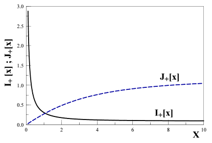

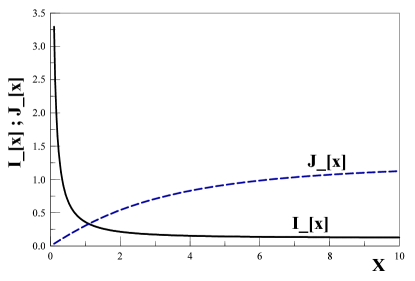

These figures make clear that the onset of the non-relativistic behavior occurs for in both cases. It is useful to compare this result, with the generalized constraint eq.(60) for the case of thermal relics. Replacing the LTE distribution functions (Fermi-Dirac or Bose-Einstein, without chemical potentials) in eq.(60) we obtain
| (63) |
The detailed analysis of the corresponding functions yields the more precise estimate in both cases for the transition to the non-relativistic regime.
Therefore, the decoupled particle of mass becomes non-relativistic at a time when . At the time of Big Bang Nucleosynthesis (BBN) when kt MeV and , the decoupled particle is non-relativistic if
| (64) |
in which case it does not contribute to the effective number of ultrarelativistic degrees of freedom during BBN and would not affect the primordial abundances of light elements. If the particle remains ultrarelativistic during BBN the total energy density in radiation is kt
| (65) |
where is the (LTE) temperature of the fluid, for Bosons (Fermions), is the effective number of ultrarelativistic degrees of freedom at time from particles that remain in LTE at this time, and is the effective number of degrees of freedom at decoupling. The second term in eq.(65) is an extra contribution to the effective number of ultrarelativistic degrees of freedom.
At the time of BBN, kt and early decoupling of the light particle, , leads to a negligible contribution to the effective number of ultrarelativistic degrees of freedom well within the current bounds verde . Therefore, provided that the decoupled particle is stable, either for light particles that remain relativistic during (BBN) but that decouple very early on when or when the particle’s mass MeV, there is no influence on the primordial abundance of light elements and BBN does not provide any tight constraints on the particle’s mass.
III.2 A Bose condensed light particle as a Dark Matter component
Consider the case of a light bosonic particle, for example an axion-like-particle. Typical interactions involve two types of processes, inelastic reactions are number-changing processes and contribute to chemical equilibration, while elastic ones distribute energy and momenta of the intervening particles, these do not change the particle number but lead to kinetic equilibration. Consider the case in which chemical freeze out occurs before kinetic freeze-out, such is the case for a real scalar field with quartic self-interactions. In this theory, number-conserving processes such as establish kinetic (thermal) equilibrium, but conserve particle number, a cross section for such process is where is the quartic coupling. The lowest order number-changing processes that contribute to chemical equilibrium are , with cross sections . Hence this is an example of a theory in which chemical freeze out occurs well before kinetic freeze out for small coupling.
Another relevant example is the case of WIMPs studied in ref. dominik where it was found that , while where are the chemical and kinetic (thermal) decoupling temperatures respectively. Although this study focused on a fermionic particle, it is certainly possible that a similar situation, namely chemical freeze-out much earlier than kinetic freeze out, may arise for bosonic DM candidates.
Under this circumstance, the number of particles is conserved if the particle is stable, but the temperature continues to redshift by the cosmological expansion, therefore the gas of Bosonic particles cools at constant comoving particle number. This situation must eventually lead to Bose Einstein condensation (BEC) since the thermal distribution function can no longer accomodate the particles with non-vanishing momentum within a thermal distribution. Once thermal freeze out occurs, the frozen distribution must feature a homogeneous condensate and the number of particles for zero momentum becomes macroscopically large. Although some aspects of Bose Einstein condensates were studied in ref. madsenQ ; madsenbec , we study new aspects such as the impact of the BEC upon the bound for the mass and the velocity dispersion of DM candidates.
The bosonic distribution function for a fixed number of particles includes a chemical potential and is given by eq.(17) where for the distribution function to be manifestly positive for all . Separating explicitly the contribution from the mode the number of particles per comoving volume is
| (66) |
where
| (67) |
is the comoving condensate density. In the infinite volume limit the condensate term vanishes unless . For we find
| (68) |
where
| (69) |
The maximum value that can achieve is , therefore, neglecting we replace by . If the comoving particle density
| (70) |
then, there must be a zero momentum condensate with and in the infinite (comoving) volume limit. In this limit we find,
| (71) |
where the critical temperature is given by
| (72) |
The solution of the equation (66) that determines the condensate fraction shows that for
| (73) |
In the infinite volume limit the distribution function for particles that decouple while ultrarelativistic , for becomes
| (74) |
From eq.(25) the total number of particles for is given by
| (75) |
where
| (76) |
For eq.(71) implies that
| (77) |
hence for the total density is given by
| (78) |
The enhancement factor over the thermal result reflects the population of particles in the condensed, zero momentum state. The energy density and pressure are given by
| (79) | |||||
| (80) |
where
| (81) | |||||
| (82) |
are the contributions from the particles outside the condensate ().
Two important aspects emerge from these expressions: i) the condensate always contributes as a non-relativistic component, ii) the condensate does not contribute to the pressure.
Replacing eq.(77) into (79) and using
the energy density and equation of state for can be written compactly as
| (83) |
where
| (84) |
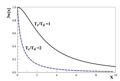
The equation of state
| (85) |
is displayed in fig. 3, from which it is clear that for the non-relativistic limit sets in much earlier than for the non-Bose condensed case. This is a consequence of the zero momentum particles in the BEC which contribute as pressureless cold matter, even when the light bosonic particle decouples while ultrarelativistic.
For when the particle becomes non-relativistic, namely , the energy density becomes
| (86) |
where is the total number of particles per physical volume, including the condensate and non-condensate components, from eq.(78) it follows that
| (87) |
from which for it follows analogously to eq.(56) that
| (88) |
The dark matter fraction that these particles can contribute is given by
| (89) |
resulting in the upper bound
| (90) |
In the Bose condensed case the bosonic particle is light unless it decouples very early on at high temperature with a large . The presence of a BEC tightens the constraint on the mass of the light bosonic particle via the extra factor in (90).
Of importance for clustering, is the velocity dispersion when the particle becomes non-relativistic, it is given by
| (91) |
where .
The presence of the BEC, accounted for by the factor in eq.(91), diminishes the velocity dispersion. This is a consequence of the fact that the particles in the condensate all have vanishing momentum, and only the non-condensate particles contribute to the velocity dispersion but the fraction of particles outside of the condensate is precisely the factor . Therefore the presence of a BEC leads to a decrease in the velocity dispersion and consequently even for light particles to a decrease in the free streaming length.
These results imply that although the Bosonic particle is bound to be very light by the bound (90) (unless they decoupled very early ), if it is not a HDM component but can effectively act as either a WDM or CDM because of a small velocity dispersion. Whether or not has to be studied within the microscopic particle physics model that describes this DM component.
IV Coarse grained phase space densities and new DM Bounds
In their seminal article Tremaine and Gunn TG argued that the coarse grained phase space density is always smaller than or equal to the maximum of the (fine grained) microscopic phase space density, which is the distribution function. Such argument relies on the theorem theo that states that collisionless phase mixing or violenty relaxation by gravitational dynamics can only diminish the coarse grained phase space density. A similar argument was presented by Dalcanton and Hogan dalcanton1 ; hogan , and confirmed by recent numerical studies numQ .
As noticed in ref. madsenQ , the case of the Bose-Einstein distribution, requires a careful treatment because for massless particles the Bose-Einstein distribution diverges at small momentum. This divergence is present if there is a BEC even when the mass of the Bosonic particle is included. This is so since is required to form a BEC and the distribution functions diverge at zero momentum, even the part of the distribution function that describes the particles outside the condensate diverges at . Madsen recognized this caveat in the Bosonic case and in ref. madsenQ introduced an alternative statistical interpretation of the phase space density, similar to that introduced in dalcanton1 ; hogan but with the upper limit in the momentum integrals replaced by a (physical) momentum cutoff as suggested by the phase mixing theorem theo . However, it is straightforward to show that the resulting coarse grained phase space density is not a Liouville invariant. Instead, we define the coarse grained (dimensionless) primordial phase space density
| (92) |
which is Liouville invariant and where is defined in eq.(52). Since the distribution function is frozen and is a solution of the collisionless Boltzmann (Liouville) equation (14) it is clear that is a constant, namely a Liouville invariant in absence of self-gravity, . Including explicitly a possible BEC, is given by
| (93) |
where is the distribution function for the non-condensed particles in the Bosonic case and is the comoving density of the Bose-Einstein condensate
| (94) |
When the particle becomes non-relativistic and , therefore,
| (95) |
where is the phase-space density introduced by Dalcanton and Hogan dalcanton1 ; hogan
| (96) |
and the one-dimensional velocity dispersion is defined by eq.(53).
In the non-relativistic regime is related to the coarse grained phase space density introduced by Tremaine and Gunn TG
| (97) |
The observationally accessible quantity is the phase space density , therefore, using for a decoupled particle that is non-relativistic today and eq.(53), we define the primordial phase space density
| (98) |
where we used that .
During collisionless gravitational dynamics, phase mixing increases the density and velocity dispersions in such a way that the coarse grained phase space density either remains constant or diminishes, namely
| (99) |
where is given by eq.(93) for an arbitrary distribution function. For a particle that decouples when it is ultrarelativistic does not depend on the mass, hence eq.(99) yields a lower bound on the mass of the particle directly from the observed phase space density and the knowledge of the distribution function.
For comparison it is convenient to gather the values eq.(93) for the usual LTE cases that follow from eqs.(34) and (38)
| (100) |
where is the number of ultrarelativistic degrees of freedom at decoupling.
We note that for the presence of a BEC increases dramatically the primordial phase space density. This is a consequence of the enhancement of the particle density over the thermal case due to the presence of the condensate, and the decrease in the velocity dispersion because the particles in the condensate all have zero momentum.
IV.1 New bounds from phase space density and dShps-data
We derive here new bounds from the latest compilation presented in ref. gilmore directly on for the dataset comprising ten satellite galaxies in the Milky-Way dSphs. It proves convenient to write eq.(99) as
| (101) |
the data in ref. gilmore yields the range
| (102) |
and we choose a fiducial value for this quantity in the middle of the range of the data gilmore , leading to the new bound
| (103) |
For thermal relics that decoupled while ultrarelativistic with vanishing chemical potentials and no BEC, we find from eqs.(100) and (103),
| (104) |
and for Bosons with BEC () we find
| (105) |
For particles that decouple out of LTE with arbitrary distribution functions the form of the new bound is given by eq.(103) with given by eq.(93). The detailed form of is completely determined by the distribution function at decoupling, which must be obtained from a microscopic calculation of the kinetics of decoupling. Once the distribution function is obtained, the new bound eq.(103) yields the lower bound of the mass consistent with the observational data.
Combining the upper bound (58) with the lower bound eq.(101) we establish the mass range for the DM candidate
| (106) |
where is given by eq.(93) and the compilation of data in gilmore constrains the bracket .
For thermal relics that decoupled in LTE while ultrarelativistic, and taking the bracket in the middle of the range we obtain from eqs.(100) and (106)
| (107) |
Therefore, if the thermal relic decouples in equilibrium this mass range indicates that it must decouple when , namely at or above the electroweak scale kt . In the BEC case, for the fulfillment of the bound requires very large , namely thermal decoupling at a scale much larger than the electroweak scale.
An alternative is that the particle is very weakly coupled to the plasma and decouples away from equilibrium with a distribution function that yields a smaller abundance increasing the right hand side of eqn. (107 ).
IV.2 Generalized Tremaine-Gunn bound.
The Tremaine-Gunn bound TG establishes a relation between the properties of dark matter in galaxies through their phase space densities. It assumes that dark matter could be reliably described by an isothermal sphere solution of the Lane-Emden equation with the equation of state (53) bt ; gas . In thermal equilibrium the quantity gas
| (108) |
is bound to be to prevent the gravitational collapse of the gas. Here stands for the volume occupied by the gas, for the number of particles and for the gas temperature. The length is similar to the King radius bt . However, the King radius follows from the singular isothermal sphere solution while is the characteristic size of a stable isothermal sphere solution gas .
Combining eq.(108) with eq.(99) results in a generalized Tremaine-Gunn bound
| (109) |
therefore the generalized Tremaine-Gunn bound on the mass becomes
| (110) |
The compilation of recent photometric and kinematic data from ten Milky Way dSphs satellites gilmore yield values for the one dimensional velocity dispersion and the radius () in the ranges
| (111) |
For particles that decouple in LTE when they are ultrarelativistic (ultrarelativistic thermal relics) with vanishing chemical potential and no BEC we find from eqs.(100) and (110),
| (112) |
For the case of ultrarelativistic bosonic thermal relics with a BEC and we find the bound
| (113) |
Therefore, the BEC case allows for smaller masses to saturate the Tremaine-Gunn bound for , a consequence of the enhanced primordial phase space density in the presence of the BEC.
IV.3 DM mass values from velocity dispersion
We can use the independent data provided in ref. gilmore on the mean density and velocity dispersion to explore bounds solely from the velocity dispersion. Since the phase space density only diminishes or remains constant during the collisionless gravitational dynamics of clustering, from which it follows that
| (114) |
where and are, respectively, the matter density and velocity dispersion of the homogeneous dark matter prior to gravitational collapse. and are, respectively, the satellite’s mean volume mass density and velocity dispersion. Assuming that DM has a single component, its density today is pdg
| (115) |
is given by eq.(54). Ref. gilmore quotes the following values for the favored satellite’s cored dark matter density and velocity dispersion
| (116) |
Eqs. (114), (115) and (116) lead to
| (117) |
Combining eq.(54) for and eq.(117) yields
| (118) |
For thermal fermions or bosons without chemical potential (no BEC) and we find in agreement with the bounds found above and the conclusions of ref. faber . A suppression factor appears in the BEC case for the same range of .
We emphasize that the bound eq.(118) is independent from the bound eq.(104) obtained from the phase space density above, and relies on the fact that the observational data gilmore yields separate information on and .
It proves illuminating to analyze the velocity dispersion from expression (54) at for thermal relics. We find
| (119) |
We see that for light Bosonic particles that decoupled while ultrarelativistic but undergo BEC can effectively act as CDM with very small velocity dispersion.
In ref. dominik it is found that kinetic decoupling for a WIMP of mass occurs at , leading to the estimate . Thus, for CDM from weakly interacting massive particles the velocity dispersion eq.(119) is:
| (120) |
Thus, is eight orders of magnitude smaller than the typical velocity dispersion in dSphs gilmore for wimps of GeV that decoupled in LTE at dominik .
It is noteworthy to compare the phase space densities of the homogeneous dark matter distribution for the thermal relics that decoupled ultrarelativistically and non-relativistically with that observed in the satellites dShps. If the distribution of dark matter is cored gilmore 111
| (121) |
If the distribution of dark matter is cusped, ref. gilmore gives the value for the density yielding
| (122) |
Assuming that a thermal relic that decoupled when ultrarelativistic is the only DM component with the density given by the value today pdg , we find from eqs.(54) at ,
| (123) |
Thus, for we see that for the phase space density for thermal relics that decoupled being ultrarelativistic is of the same order as the phase space density in dShps with cores, eq.(121). Thermal relics with mass in the range obviously favor cores over cusps because the primordial phase space is for cores while for a cuspy distribution, and according to the theorem in theo ; TG , the phase space density can only diminish during gravitational clustering.
An enhancement factor appears in eq.(123) for the case of a BEC. Notice, that for and , a BEC yields a phase space density consistent with cusps as a result of the small velocity dispersion and the CDM behavior.
Recent -body simulations numQ indicate that the phase space density decreases by a factor due to gravitational relaxation during structure formation between , with smaller relaxation in WDM than in CDM numQ ; dalcanton1 . Therefore, from these numerical results it follows that
| (124) |
Combining this result with the observational results eqs.(121)-(122) and the primordial phase space density eq.(123) for a thermal relic that decoupled while ultrarelativistic, we find
| (125) |
These values and the upper bounds for in eqs.(107) yield the following bounds for thermal relics
| (126) |
Therefore, thermal relics, DM candidates that decouple when relativistic, must decouple at a temperature well above the electroweak scale. Eqs.(125) and (126) imply for the mass value:
| (127) |
Although is not too much larger than it is noteworthy that the thermal relic DM candidate that leads to cusped profiles must decouple when namely very early at a temperature scale corresponding to a grand unified theory with a large symmetry group.
For the case of CDM from wimps which decoupled non-relativistic, we find from eqs.(115) and (119)
| (128) |
The phase space density always decreases by dynamical relaxation, a result recently confirmed numerically by -body simulationsnumQ . For initial values of the phase space density which are much lower than the primordial ones, these yield a typical decrease by a factor numQ . If these results should persist in N-body simulations with larger values of the initial phase space density, they would imply a tension between the phase space density of WIMPs eq.(128) being eighteen to fifteen orders of magnitude larger than that in dShps either cored eq.(121) or cusped eq.(122)gilmore .
¿From the combined analysis of the primordial phase space densities, the observational data on dSphs gilmore and the -body simulations in ref. numQ , we conclude the following:
-
•
(i): Thermal relics with few keV that decouple when ultrarelativistic lead to a primordial phase space density of the same order of magnitude as in cored dShps and disfavor cusped satellites for which the data gilmore yields a much larger phase space density.
-
•
(ii): Light bosonic particles decoupled while ultrarelativistic and which form a BEC lead to phase space densities consistent with cores and if , also consistent with cusps. However, for thermal relics to satisfy the bound eq.(107) they must decouple when , namely above the electroweak scale. Recall that typically takes a value between one and four.
V Non-equilibrium effects:
The main results of our analysis are the new bounds from DM abundance and phase space density of dShps summarized in eq.(106). When the dark matter candidate decouples out of LTE these bounds establish a direct connection with the microphysics via the frozen distribution functions. These functions must be obtained from a detailed calculation of the microscopic processes that describe the production and pathway towards equilibration of the corresponding dark matter candidate. If kinetic (and chemical) freeze out occur out of LTE the distribution functions will keep memory of the initial state and the detail of the processes that established it.
Non-equilibrium effects have been mainly considered for massive particles that decoupled when non-relativistic steenneq or as distortions in the neutrino distribution functions during BBN manga ; kawa . Instead, we focus here on DM constraints from decoupling out of (LTE) at temperatures larger than the BBN scale and when particles are ultrarelativistic. Decoupling out of LTE in this case has been much less studied. In this section we explore a cosmologically relevant mechanism of production and equilibration which describes a wide variety of situations out of LTE.
V.1 Particle production followed by an UV cascade:
Early studies of particle production via parametric amplification and oscillations of inflaton-like scalar fields revealed that particles are produced via this mechanism primarily in a low momentum band of wave vectors boydata leading to a non-thermal spectrum (figs. 2-3 in ref. boydata illustrate these effects).
Subsequent studies dvd showed that the early phase of parametric amplification and particle production is followed by a long stage of mode mixing and scattering that redistributes the particles: the larger momentum modes are populated by a cascade whose front moves towards the ultraviolet akin to a direct cascade in turbulence, leaving in its wake a state of nearly LTE but with a lower temperature than that of equilibrium dvd .
The dynamics during the cascade process diminishes the amplitude of the distribution function at lower momenta and populates the higher momentum modes. The distribution function develops a front that moves towards the ultraviolet. Behind the front the distribution function is nearly that of LTE with a different temperature and amplitude and slowly evolves towards thermal equilibrium dvd . If these particles are very weakly coupled to the plasma it is possible that the advance of the cascade and the front of the distribution towards larger momenta is interrupted when the rate of scattering or mode mixing becomes smaller than the expansion rate. In this case, the distribution function is frozen well before reaching complete LTE resulting in a population of modes primarily at lower momenta up to the scale of the front. This study dvd suggests the following frozen distribution function
| (130) |
where is the equilibrium distribution function for an ultrarelativistic particle at an effective temperature . Namely, at thermal equilibrium and before thermodynamical equilibrium is attained.
This form describes fairly accurately the cascade with a front that moves towards the ultraviolet, which is interrupted at a fixed value of the momentum, identified here to be ; is the temperature of the environmental degrees of freedom that are in LTE at the time of decoupling.
The amplitude and effective temperature reflect an incomplete thermalization behind the front of the cascade and determine the average number of particles in its wake dvd . This interpretation is borne out by the detailed numerical studies in ref. dvd . For Fermi-Dirac ultrarelativistic particles (with vanishing chemical potential) whereas for Bose-Einstein ultrarelativistic particles . Neglecting the possibility of a BEC, for a fermionic or bosonic equilibrium distribution function , we find
| (131) | |||
| (132) | |||
| (133) |
and the primordial phase space density becomes
| (134) |
where is the phase space density eq.(93) for the equilibrium distribution .
For a fermionic species without chemical potential [], the bound eq.(106) becomes
| (135) |
and the one dimensional velocity dispersion eq.(54) becomes today:
| (136) |
The functions and for the case are displayed in fig. 4. For the Bose-Einstein case without a BEC the behaviors of and are qualitatively similar.
It is clear that the bound eq.(135) for the range of can easily be satisfied for moderate values corresponding to decoupling temperatures and .


Remarkably, the non-equilibrium distribution eq.(130) turns out to be a generalization of several non-equilibrium distribution functions of cosmological relevance proposed in the literature:
-
•
(a): sterile neutrinos produced non-resonantly via the Dodelson-Widrow mechanism dw for which the distribution function is obtained from (130) by taking (ref. dw ). In this case we find for the mass range, phase space density and velocity dispersion respectively,
(137) The major uncertainty is the evaluation of . In the Dodelson-Widrow dw scenario the sterile neutrino production peaks at , this temperature is very near the region where the QCD phase transition occurs at which the effective number of ultrarelativistic degrees of freedom changes dramatically. If decoupling occurs at a temperature higher than the QCD critical temperature, then and the mass bound eq.(137) may be fulfilled, but for a lower decoupling temperature when the mass bound may not be fulfilled. If the mass bound is fulfilled, is compatible with cored dSphs gilmore [see eq.(121)] but not with the cusped distributions, [see eq.(122)]. Combining the bound eq.(137), the observed phase space density eq.(121) gilmore and the -body results of ref. numQ which yield phase space relaxation by a factor we find that
(138) -
•
(b): sterile neutrinos produced by a net-lepton number driven resonant conversion studied by Shi and Fuller este for which the distribution function is obtained from eq.(130) for , (see fig. 1 in the first reference in este ). We find
(139) Again, a source of uncertainty is the evaluation of , because in the resonant-mediated sterile neutrino production, the maximum production rate is near the QCD temperature este . However, it is clear that in this case the mass bound is less sensitive to the uncertainty in (a small value fulfills the bound), although the MSW resonance occurs also near the QCD critical temperature este . The velocity dispersion is small because the distribution is skewed towards small momenta. Again, is consistent with cored dSphs [see eq.(121)] but not with cusped distributions [see eq.(122)]. A similar analysis as in the previous case combining the observational data, the results of ref. numQ and the bound eq.(139) yields
(140) - •
Although recent studies boyho suggest that the description of the production mechanism of sterile neutrinos must be reassessed with likely implications on their distribution functions after decoupling, the above estimates provide a guidance to the range of mass, primordial phase space density and velocity dispersions for sterile neutrinos as possible WDM candidates.
VI Conclusions
We have obtained new constraints on light DM candidates that decoupled while ultrarelativistic in or out of LTE in terms of their distribution functions. The only assumption is that these distribution functions are homogeneous and isotropic. A Liouville invariant coarse grained primordial phase space density is introduced that allows to combine phase space density arguments with a recent compilation of photometric and kinematic data on dSphs galaxies to yield new constraints on the mass, velocity dispersion and phase space density of DM candidates. The new constraint on the mass range is
| (142) |
where the primordial phase space density is given by
| (143) |
is the distribution function at decoupling, the number of internal degrees of freedom of the particle, and is the phase space density obtained from observations. The upper bound arises from requesting that the DM candidate has a density today, and the lower bound arises from requesting that the phase space density in halos be smaller than or equal to the primordial phase space density of the collisionless non-relativistic (today) DM component
We have studied the consequences of Bose-Einstein condensation of light ultrarelativistic particles when chemical freeze out occurs well before kinetic decoupling at with the critical temperature below which a non-vanishing condensate fraction exists. We find that the presence of the condensate hastens the onset of the non-relativistic regime and that Bose-Einstein condensed particles can effectively act as a CDM component even when they decoupled being ultrarelativistic. The reason for this unusual behavior is that the particles in the condensate all have vanishing velocity dispersion.
For thermal relics we find
| (144) |
The combination of data in ref. gilmore from dSphs when applied to light thermal relics yields the mass range
| (145) |
with the implication that if these particles are suitable DM candidates, they must decouple at high temperature when the effective number of ultrarelativistic degrees of freedom is . Namely, in absence of a BEC, thermal decoupling must occur above the electroweak scale. In the BEC case, for , the fulfillment of the bound requires very large . Namely, in the presence of a BEC thermal decoupling occurs at a scale much larger than the electroweak scale for .
Assuming that the DM particle is the only component with the density today, we obtained an independent bound from velocity dispersion which for the favored cored profiles gilmore yield the lower mass bound
| (146) |
For light thermal relics this bound implies that with a suppression factor in the BEC case.
For light thermal relics that decoupled while ultrarelativistic we find the primordial phase space density
| (147) |
An enhancement factor appears in the r.h.s. in the presence of a BEC.
For wimps with kinetic decoupling temperature MeV dominik , we find
| (148) |
The observational data compiled in ref. gilmore assuming a favored cored profile suggests
| (149) |
If the distribution of dark matter is cusped, ref. gilmore gives the value for the density yielding
| (150) |
Therefore, for the primordial phase space density for thermal relics with favors a cored distribution.
Notice that a bosonic thermal relic that features a BEC can behave as CDM with small velocity dispersion and a primordial phase space density consistent with cusped distributions if . However, these BEC DM candidates must decouple at a temperature scale higher than the electroweak.
Recent results from -body simulations suggests that the phase space density relaxes by a factor during gravitational clustering for numQ . Combining these numerical results with the observational results on dSphs gilmore and the present DM density, we conclude that the mass of thermal relics that decoupled when ultrarelativistic is
| (151) |
The decoupling temperature for the DM candidate that would favor cusped profiles must be near a grand unified scale for a large symmetry group with which effectively results in a colder relic today with a far smaller velocity dispersion.
The enormous discrepancy between the primordial phase space density for WIMPs of , eq.(148) and the phase space densities in dSphs, either cored (eq.149 ) or cusped (eq.150) cannot be explained by the two orders of magnitude of gravitational relaxation of phase space densities found with recent -body simulations numQ , although these initialize the simulation with much smaller values of the primordial phase space density.
We have studied a scenario for decoupling out of equilibrium motivated by previous studies of particle production and thermalization via an UV cascade. The distribution function obtained from previous studies dvd , remarkably describes the non-equilibrium distribution functions for sterile neutrinos produced either resonantly este or non-resonantly dw as well as a recently proposed model for halo structure strigari . Our bounds in terms of arbitrary distribution functions lead to the following bounds on the mass, phase space density and velocity dispersion of these light relics that decoupled out of LTE:
-
•
For sterile neutrinos produced non-resonantly via the Dodelson-Widrow mechanism dw we find
(152) The upper and lower bound on the mass can only be compatible if the sterile neutrino decouples with . For the primordial phase space density is compatible with cored but not with cusped profiles in the dShps data gilmore . Combining these bounds with the results from -body simulations on the relaxation of the phase space density numQ and with the observational constraint eq.(121) gilmore , we obtain the value
(153) for the mass of sterile neutrinos produced non-resonantly by the Dodelson-Widrow mechanism.
-
•
For sterile neutrinos produced by a net-lepton number driven resonant conversion este we find
(154) The small velocity dispersion is a consequence of the distribution function being skewed towards small momentum. Again for , the primordial phase space density is compatible with cored but not cusped profiles in the dShps data gilmore . For sterile neutrinos produced by resonant conversion, a similar analysis as for the previous case yields
(155) -
•
For the model proposed in ref. strigari we find
(156)
It is noteworthy that the -body results of ref. numQ which yield phase space relaxation by a factor bring the values of the primordial phase space density of the above cases within the range consistent with the phase space densities for cored profiles in dSphs gilmore for . On the contrary, in the case of WIMPs with , relaxation by many orders of magnitude is necessary for their phase space densities to be compatible with the observed values both for cores and for cusps.
Therefore the bounds eqs.(153)-(155) confirm that relics that decouple out of equilibrium while ultrarelativistic via the mechanisms described above yield values for phase space densities that are in agreement with cores in the DM distribution.
The results obtained in this article for the new mass bounds, primordial phase space densities and velocity dispersion in term of arbitrary, but homogeneous and isotropic distribution functions establish a link between the microphysics of decoupling and observable quantities. They also warrant deeper scrutiny of the non-equilibrium aspects of sterile neutrinosboyho for a firmer assessment of their potential as DM candidates.
Acknowledgements.
We thank Carlos Frenk, for useful discussions, D.B. thanks Andrew Zentner for fruitful discussions, and acknowledges support from the U.S. National Science Foundation through grant award PHY-0553418.References
- (1) F. Zwicky, Helv. Phys. Acta, 6, 124 (1933), Phys. Rev. 51, 290 (1937); J. H. Oort, ApJ, 91, 273 (1940).
- (2) See for example, J. Primack, New Astron.Rev. 49, 25 (2005); arXiv:astro-ph/0609541, and references therein.
- (3) G. Kauffman, S. D. M. White, B. Guiderdoni, Mon. Not. Roy. Astron. Soc. 264, 201 (1993).
- (4) S. Ghigna et.al. Astrophys.J. 544,616 (2000).
- (5) B. Moore et. al., Astrophys. J. Lett. 524, L19 (1999).
- (6) A. Klypin et. al. Astrophys. J. 523, 32 (1999).
- (7) J. Dubinski, R. Carlberg, Astrophys.J. 378, 496 (1991).
- (8) J. F. Navarro, C. S. Frenk, S. White, Mon. Not. R. Astron. Soc. 462, 563 (1996).
- (9) J. S. Bullock et.al., Mon.Not.Roy.Astron.Soc. 321, 559 (2001); A. R. Zentner, J. S. Bullock, Phys. Rev. D66, 043003 (2002); Astrophys. J. 598, 49 (2003).
- (10) J. Diemand et.al. Mon.Not.Roy.Astron.Soc. 364, 665 (2005).
- (11) J. J. Dalcanton, C. J. Hogan, Astrophys. J. 561, 35 (2001).
- (12) F. C. van den Bosch, R. A. Swaters, Mon. Not. Roy. Astron. Soc. 325, 1017 (2001).
- (13) R. A.Swaters, et.al., Astrophys. J. 583, 732 (2003).
- (14) R. F.G. Wyse and G. Gilmore, arXiv:0708.1492; G. Gilmore et. al. arXiv:astro-ph/0703308.
- (15) O. E.Gerhard, D. N. Spergel, Astrophys. J. 389, L9, (1992).
- (16) F. C. van den Bosch et. al. Astron. J. 119, 1579 (2000).
- (17) B. Moore, et.al. Mon. Not. Roy. Astron. Soc. 310, 1147 (1999); P. Bode, J. P. Ostriker, N. Turok, Astrophys. J 556, 93 (2001); V. Avila-Reese et.al. Astrophys. J. 559, 516 (2001).
- (18) S. Dodelson, L. M. Widrow, Phys. Rev. Lett. 72, 17 (1994).
- (19) X. Shi, G. M. Fuller, Phys. Rev. Lett. 82, 2832 (1999); K. Abazajian, G. M. Fuller, M. Patel, Phys. Rev. D64, 023501 (2001); K. Abazajian, G. M. Fuller, Phys. Rev. D66, 023526, (2002); G. M. Fuller et. al., Phys.Rev. D68, 103002 (2003); K. Abazajian, Phys. Rev. D73,063506 (2006); M. Shaposhnikov, I. Tkachev, Phys. Lett. B639,414 (2006).
- (20) A. Kusenko, arXiv:hep-ph/0703116; arXiv:astro-ph/0608096; T. Asaka, M. Shaposhnikov, A. Kusenko; Phys.Lett. B638, 401 (2006); P. L. Biermann, A. Kusenko, Phys. Rev. Lett. 96, 091301 (2006);
- (21) P. B. Pal, L. Wolfenstein, Phys. Rev. D25, 766 (1982); V. D. Barger, R. J. N. Phillips, S. Sarkar, Phys. Lett. B352,365 (1995).
- (22) A. D. Dolgov and S. H. Hansen, Astropart. Phys. 16, 339 (2002); K. Abazajian, S. M. Koushiappas, Phys. Rev. D74 023527 (2006); K. Abazajian, G. M. Fuller, W. H. Tucker, Astrop. J. 562, 593 (2001); A. Boyarsky, A Neronov, O Ruchayskiy, M. Shaposhnikov, Mon.Not.Roy.Astron.Soc. 370, 213 (2006); JETP Lett. 83 , 133 (2006); Phys.Rev. D74, 103506 (2006); A. Boyarsky, A. Neronov, O. Ruchayskiy, M. Shaposhnikov, I. Tkachev,Phys. Rev. Lett. 97, 261302 (2006); A. Boyarsky, J. Nevalainen, O. Ruchayskiy, astro-ph/0610961; A. Boyarsky, O. Ruchayskiy, M. Markevitch, astro-ph/0611168; S. Riemer-Sorensen, K. Pedersen, S. H. Hansen, H. Dahle, arXiv:astro-ph/0610034; S. Riemer-Sorensen, S. H. Hansen and K. Pedersen, Astrophys. J. 644 (2006) L33;
- (23) U. Seljak et. al., Phys. Rev. Lett. 97, 191303 (2006); M. Viel et.al., Phys. Rev. Lett. 97, 071301 (2006); P. McDonald et.al. Astrophys. J. Suppl. 163, 80 (2006).
- (24) M. Viel et.al. arXiv:0709.0131 (2007).
- (25) H. Yüksel, J.F. Beacom, C. R. Watson, arXiv:0706.4084.
- (26) L. E. Strigari et.al, Astrophys.J. 652, 306 (2006).
- (27) A. Palazzo et.al., arXiv:0707.1495.
- (28) A. Boyarski, et.al. arXiv:0709.2301.
- (29) J. R. Bond, G. Efstathiou, J. Silk, Phys. Rev. Lett.45, 1980 (1980).
- (30) S. Tremaine, J.E. Gunn, Phys. Rev. Lett. 42, 407 (1979).
- (31) B W Lee, S. Weinberg, Phys. Rev. Lett. 39, 165 (1977). P Hut, Phys. Lett. B 69, 85 (1977). K. Sato, H. Kobayashi, Prog. Theor. Phys. 58, 1775 (1977). M. I. Vysotsky, A. D. Dolgov, Ya. B. Zeldovich, JETP Lett. 26, 188 (1977).
- (32) E. W. Kolb, M. S. Turner, The Early Universe , Addison-Wesley, (1990).
- (33) A. M. Green, S. Hofmann, D. J. Schwarz, JCAP 0508 003 (2005); S. Hofmann, D. Schwarz, H. Stocker, Phys. Rev. D64, 083507 (2001); A. M. Green, S. Hofmann, D. J. Schwarz, Mon. Not. Roy. Astron. Soc. 353 L23 (2004), and references therein.
- (34) G. B. Larsen, J. Madsen, Phys. Rev. D52, 4282 (1995).
- (35) J. Madsen, Phys. Rev. Lett. 69, 571 (1992).
- (36) J. Madsen, Phys. Rev. D44, 999 (1991); Phys. Rev. D64, 027301 (2001); Phys. Rev. Lett. 64, 2744 (1990).
- (37) P. Salucci, A. Sinibaldi, Astron. Astrophys. 323, 1 (1997).
- (38) C. J. Hogan, J. J. Dalcanton, Phys. Rev. D62, 063511 (2000).
- (39) J. Lesgourges, S. Pastor, Phys. Rept. 429, 307 (2006).
- (40) S. Hannestad, Ann. Rev. Nucl. Part. Sci. 56, 137 (2006).
- (41) S. Hannestad, G. Raffelt, JCAP 0404, 008(2004); S. Hannestad, A. Mirizzi, G. Raffelt, JCAP 0507, 002 (2005), S. Hannestad et.al. arXiv:0706.4198 (2007).
- (42) A. Melchiorri, O. Mena, A. Slosar, arXiv:0705.2695 (2007).
- (43) D. Lynden-Bell, Mon. Not. Roy. Astron. Soc. 136, 101 (1967), S. Tremaine, M. Henon, D. Lynden-Bell, Mon. Not. Roy. Astron. Soc. 219, 285 (1986).
- (44) S. Peirani et. al., Mon. Not.R. Astron. Soc. 367, 1011 (2006); S. Peirani, J. A. de Freitas Pacheco, astro-ph/0701292; E. Romano-Diaz et.al., Astrophys. J. 637, L93 (2006); E. Romano-Diaz et.al., Astrophys. J. 657, 56 (2007); Y. Hoffman et.al. arXiv:0706.0006.
- (45) D. Boyanovsky, M. D’Attanasio, H. J. de Vega, R. Holman, D.-S. Lee, Phys. Rev. D52, 6805 (1995).
- (46) D. Boyanovsky, C. Destri, H. J. de Vega, Phys.Rev. D69, 045003 (2004). C. Destri, H. J. de Vega, Phys.Rev. D73, 025014 (2006).
- (47) J. Bernstein, Kinetic theory in the expanding Universe, Cambridge University Press, N.Y, 1988.
- (48) S. Dodelson, Modern Cosmology, Academic Press, London, (2003).
- (49) W.-M. Yao et al., Journal of Physics G 33, 1 (2006).
- (50) R. Cowsick and J. McClelland, Phys. Rev. Lett. 29, 669 (1972).
- (51) D. Boyanovsky,(to be submitted).
- (52) D. Spergel et.al. (WMAP collaboration), ApJS, 170, 377 (2007).
- (53) S. Hansen, et. al., Phys. Rev. D65, 023511 (2001); J. P. Kneller et.al. Phys. Rev. D64, 123506 (2001).
- (54) F. de Bernardis et. al., arXiv:0707.4170; G. Mangano et. al., JCAP 0703, 006 (2007).
- (55) J. Binney, S. Tremaine, Galactic Dynamics, Princeton University Press, 1987.
- (56) H. J. de Vega, N. Sánchez, Nuclear Physics B 625, 409 and 460 (2002). C. Destri, H. J. de Vega, Nucl. Phys. B 763, 309 (2007).
- (57) D. N. C. Lin, S. M. Faber, Astroph.J. 266, L21 (1983). J. Madsen, R. I. Epstein, Ap. J. 282, 11 (1984).
- (58) S. Hannestad, New Astron. 4, 207 (1999).
- (59) G. Mangano et.al. Nucl.Phys. B729 , 221 (2005).
- (60) K. Ichikawa, M. Kawasaki, F. Takahashi, Phys.Rev.D72 043522 (2005).
- (61) D. Boyanovsky, C.-M.Ho, Phys. Rev. D75, 085004 (2007); JHEP 07 (2007) 030; arXiv:0705.0703 (to appear in Phys. Rev. D), D. Boyanovsky, arXiv:0706.3167 (to appear in Phys. Rev. D).