Absolute FKBP binding affinities obtained via non-equilibrium unbinding simulations

Abstract

We compute absolute binding affinities for two ligands bound to the FKBP protein using non-equilibrium unbinding simulations. The methodology is straight-forward, requiring little or no modification to many modern molecular simulation packages. The approach makes use of a physical pathway, eliminating the need for complicated alchemical decoupling schemes. Results of this study are promising. For the ligands studied here the binding affinities are typically estimated within less than 4.0 kJ/mol of the target values; and the target values are within less than 1.0 kJ/mol of experiment. These results suggest that non-equilibrium simulation could provide a simple and robust means to estimate protein-ligand binding affinities.

I Introduction

The accurate estimation of binding affinities for protein-ligand systems ($\Delta G$) remains one of the most challenging tasks in computational biophysics and biochemistry Chipot and Pohorille (2007). Due to the high computational cost of such free energy computation, it is of interest to understand the advantages and limitations of various $\Delta G$ methods.

Many previous studies Bash et al. (1987); Hermans and Wang (1997); Gilson et al. (1997); Chen et al. (2004); Helms and Wade (1998); Oostenbrink et al. (2000); Dixit and Chipot (2001); Banavali et al. (2002); Boresch et al. (2003); Oostenbrink and van Gunsteren (2003); Swanson et al. (2004); Fujitani et al. (2005); Pearlman (2005); Carlsson and Aqvist (2005); Woo and Roux (2005); Deng and Roux (2006); Wang et al. (2006); Mobley et al. (2006); Jayachandran et al. (2006); Lee and Olson (2006); Mobley et al. (2007); Lee and Olson (2008) have calculated protein-ligand binding affinities using equilibrium free energy methods such as thermodynamic integration Kirkwood (1935), free energy perturbation Zwanzig (1954); Valleau and Card (1972), and weighted histogram analysis Kumar et al. (1992). Due to the introduction of the novel Jarzynski approach Jarzynski (1997a) it is also possible to estimate $\Delta G$ from non-equilibrium simulations. However, the estimation of $\Delta G$ for protein-ligand binding using non-equilibrium approaches remains largely untested. Two recent studies used non-equilibrium simulations to test unbinding pathways Zhang et al. (2006); Vashisth and Abrams (2008). Studies by other groups found that estimating $\Delta G$ via non-equilibrium simulations resulted in a large error compared to experiment Gräter et al. (2006); Cuendet and Michielin (2008). A recent study by Kuyucak and collaborators demonstrated that use of non-equilibrium simulation required longer simulation times than umbrella sampling Bastug et al. (2008).

In this report, apparently for the first time, we demonstrate the ability to compute accurate (as compared to experimental data) protein-ligand binding $\Delta G$ estimates following a non-equilibrium methodology. The approach relies on performing multiple non-equilibrium unbinding simulations using a physical pathway, i.e., pulling the ligand out of the binding pocket, and then uses the Jarzynski relation Jarzynski (1997a) to estimate $\Delta G$. The system is an FKBP protein complexed with 4-hydroxy-2-butanone (BUQ) and dimethyl sulfoxide (DMSO). The motivation for using this system is that comparison to experiment is possible Burkhard et al. (2000) and many previous computational studies have been performed Swanson et al. (2004); Fujitani et al. (2005); Jayachandran et al. (2006); Wang et al. (2006); Lee and Olson (2006).

The importance of pursuing non-equilibrium methods such as used in this report is three-fold: (i) The approach is trivially parallelizeable since each non-equilibrium unbinding simulation is performed independently. (ii) The method is simple to implement in many existing simulation packages such as GROMACS Van Der Spoel et al. (2005), used here; little or no modification to the code is necessary. (iii) Since a physical pathway is utilized, there is no need to use alchemical decoupling schemes.

This study represents the first stage of a project comparing the efficiencies of various free energy methods for protein-ligand $\Delta G$ computation. We note that efficiency studies have been carried out for other non-protein systems Radmer and Kollman (1997); Kofke and Cummings (1997); Hummer (2001); Shirts and Pande (2005); Oostenbrink and van Gunsteren (2006); Ytreberg et al. (2006).

II Theory

In general, the absolute binding affinity is defined as the free energy difference between the unbound (apo) and bound (holo) states of the protein-ligand system. We define the apo state as when the protein and ligand are not interacting due to a large separation between them. The holo state is defined to be when the ligand is in the binding pocket of the protein. Experimentally, the binding affinity is measured by determining the equilibrium constant $K_{\text{eq}}=[PL]/[P][L]$, where $[PL]$ denotes the concentration of the protein-ligand complex, and $[P]$ and $[L]$ are the concentrations of the apo protein and free ligand, respectively. Then the absolute binding affinity is given by $\Delta G_{\text{bind}}=-k_{B}T\ln(K_{\text{eq}}/V_{0})$, where $k_{B}$ is the Boltzmann constant, $T$ is the system temperature, and $V_{0}$ is the standard volume used for the experiment (typically $V_{0}=1.661$ nm² corresponding to 1.0 mol/liter concentration).

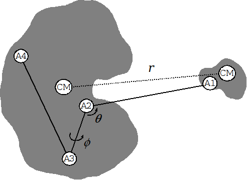
Figure 1: The coordinate system used for the restraints $U_{\text{a}}(\theta,\phi)$ and $U_{\text{r}}(r,t)$. The value of $r$ is given by the center of mass separation between the protein and ligand. A1-A4 are the heavy atoms used to define the coordinate system for $U_{\text{a}}$. For the FKBP-DMSO system A1 = DMSO:S1, A2 = TRP59:N, A3 = HIS25:N and A4 = ALA64:N. For the FKBP-BUQ system A1 = BUQ:C2, and A2-A4 are the same as FKBP-DMSO.

Following the notation of Roux and collaborators Woo and Roux (2005); Wang et al. (2006) (also see discussion in Refs. Chipot and Pohorille, 2007; Gilson et al., 1997; Boresch et al., 2003) the equilibrium constant is given by a ratio of integrals over the apo and holo regions of configurational space

$$K_{\text{eq}}=\frac{\int_{\text{holo}}d\vec{x}\int d\vec{X}\;e^{-\beta U(\vec{x},\vec{X})}}{\int_{\text{apo}}d\vec{x}\;\delta(\vec{r}-\vec{r}_{*})\int d\vec{X}\;e^{-\beta U(\vec{x},\vec{X})}}\,,$$ (1)

where $\beta=1/k_{B}T$, $\vec{x}$ represents the configurational coordinates of the ligand, $\vec{X}$ are the coordinates of the protein and solvent, and $U(\vec{x},\vec{X})$ is the potential energy of the system. The vector $\vec{r}$ defines the location of the center of mass of the ligand relative to the center of mass of the protein (see Fig. 1), and $\vec{r}_{*}$ is a reference value taken to be when the ligand and protein are not interacting.

Equation (1) can be used to compute binding affinities using various computational strategies. In our study, we restrain the ligand relative to the protein so that the ligand remains along the binding axis. The potential energy of this axial restraint is given by $U_{\text{a}}(\theta,\phi)=\frac{1}{2}k_{a}\big{[}(\theta-\theta_{0})^{2}+(\phi-\phi_{0})^{2}\big{]}$, where $k_{a}$ is the force constant and $\theta_{0},\phi_{0}$ are reference values of the coordinates; see Fig. 1. With this restraint defined, Eq. (1) can be written as a product of dimensionless ratios of integrals

$$e^{-\beta\Delta G_{\text{bind}}} =\frac{K_{\text{eq}}}{V_{0}}\equiv I_{1}\times I_{2}\,,$$

$$I_{1} =\frac{\int_{\text{holo}}d\vec{x}\int d\vec{X}\;e^{-\beta U}}{\int_{\text{holo}}d\vec{x}\int d\vec{X}\;e^{-\beta(U+U_{\text{a}})}}\,,$$

$$I_{2} =\frac{1}{V_{0}}\;\frac{\int_{\text{holo}}d\vec{x}\int d\vec{X}\;e^{-\beta(U+U_{\text{a}})}}{\int_{\text{apo}}d\vec{x}\;\delta(\vec{r}-\vec{r}_{*})\int d\vec{X}\;e^{-\beta U}}\,,$$ (2)

where strategies for computing the terms $I_{1}$ and $I_{2}$ will be discussed below.

The first term $I_{1}\equiv e^{-\beta\Delta G^{\text{holo}}_{a}}$ in Eq. (2) corresponds to the free energy difference associated with restraining the protein to the binding axis while in the holo state. This free energy can be computed using any standard technique by performing simulations for a range of force constants from 0 to $k_{a}$. For the current study we chose to compute this free energy difference via a multi-stage Bennett approach Bennett (1976).

To determine the second term $I_{2}$ in Eq. (2) we define the potential of mean force (PMF) $\mathcal{W}$, with the restraint potential $U_{\text{a}}$ present, as a function of the scalar distance $r$

$$e^{-\beta[\mathcal{W}(r_{2})-\mathcal{W}(r_{1})]}=\frac{\int d\vec{x}\;\delta(r-r_{2})\int d\vec{X}\;e^{-\beta(U+U_{\text{a}})}}{\int d\vec{x}\;\delta(r-r_{1})\int d\vec{X}\;e^{-\beta(U+U_{\text{a}})}}\,.$$ (3)

Integrating the PMF over both apo and holo regions we can obtain

$$\int_{\text{apo}}d\vec{r}_{1}\;\delta(\vec{r}_{1}-\vec{r}_{*})\;e^{-\beta U_{\text{a}}}\int_{\text{holo}}dr_{2}\;e^{-\beta[\mathcal{W}(r_{2})-\mathcal{W}(r_{1})]}$$

$$=\frac{1}{4\pi r_{*}^{2}}\frac{\int_{\text{holo}}d\vec{x}\int d\vec{X}\;e^{-\beta(U+U_{\text{a}})}}{\int_{\text{apo}}d\vec{x}\;\delta(\vec{r}-\vec{r}_{*})\int d\vec{X}\;e^{-\beta U}}\,,$$ (4)

where we have used the fact that $\delta(r-r_{*})=4\pi r^{2}\,\delta(\vec{r}-\vec{r}_{*})$ for the apo integral since the PMF is independent of the direction of $\vec{r}$ when the ligand is not interacting with the protein. Thus $I_{2}$ can be evaluated by estimating the integral of the PMF in Eq. (4),

$$I_{2} =\frac{4\pi r_{*}^{2}}{V_{0}}\int_{\text{apo}}d\vec{r}_{1}\;\delta(\vec{r}_{1}-\vec{r}_{*})\;e^{-\beta U_{\text{a}}}\int_{\text{holo}}dr_{2}\;e^{-\beta[\mathcal{W}(r_{2})-\mathcal{W}(r_{1})]}$$

$$=\frac{4\pi r_{*}^{2}}{V_{0}}\int_{\text{apo}}r_{1}^{2}dr_{1}\cos\theta_{1}d\theta_{1}d\phi_{1}\;\frac{\delta(r_{1}-r_{*})}{4\pi r_{1}^{2}}\;e^{-\beta U_{\text{a}}(\theta_{1},\phi_{1})}\;e^{+\beta\mathcal{W}(r_{1})}\int_{\text{holo}}dr_{2}\;e^{-\beta\mathcal{W}(r_{2})}$$

$$=\frac{r_{*}^{2}}{V_{0}}\;e^{+\beta\mathcal{W}(r_{*})}\int_{\text{apo}}\cos\theta_{1}d\theta_{1}d\phi_{1}\;e^{-\beta U_{\text{a}}(\theta_{1},\phi_{1})}\int_{\text{holo}}dr_{2}\;e^{-\beta\mathcal{W}(r_{2})}.$$ (5)

Below the apo integral will be evaluated analytically and the holo integral will be evaluated using quadrature.

With our approximations above the absolute binding free energy can now be estimated via the relation

$$\Delta G_{\text{bind}} =\Delta G^{\text{holo}}_{a}-\mathcal{W}(r_{*})-k_{B}T\ln\Bigg{[}\frac{r_{*}^{2}}{V_{0}}\times$$

$$\int_{\text{apo}}\cos\theta d\theta d\phi\;e^{-\beta U_{\text{a}}(\theta,\phi)}\int_{\text{holo}}dr\;e^{-\beta\mathcal{W}(r)}\Bigg{]}.$$ (6)

This is our central theoretical result. Thus, estimating $\Delta G_{\text{bind}}$ in the current framework requires three computations: the PMF must be calculated (detailed below), $\Delta G^{\text{holo}}_{a}$ must be approximated, and the apo integral must be analytically evaluated.

One may note that a different, yet viable, non-equilibrium approach would be to set $k_{a}=0$, i.e., remove the axial restraint. This would simplify the $\Delta G_{\text{bind}}$ calculation since $\Delta G^{\text{holo}}_{a}=0$ and the apo integral would be $4\pi$ in Eq. (6), and thus only the PMF would be needed. Further, the binding axis would not need to be defined by the researcher, which would allow the ligand more flexible unbinding routes. However, there are two important advantages to using the axial restraint. Most important is that since the axial restraint limits the allowable configurational space for the ligand, the PMF converges much more quickly than with no restraint. Also, in cases where the binding pocket is not at the protein surface, or when more than one viable pathway exists, it may be advantageous, or even necessary, to define the binding path to obtain meaningful results.

II.1 Estimating the PMF

The PMF will be computed using two different approaches: the Hummer-Szabo method, and the stiff-spring approximation with the second cumulant expansion. Below we summarize these techniques.

In the Hummer-Szabo approach the PMF is estimated by performing multiple non-equilibrium pulling simulations along the reaction coordinate $r$ by using a time-dependent biasing potential $U_{\text{r}}(r,t)=k_{r}[r-(r_{0}+vt)]^{2}$, where $k_{r}$ is the force constant, $r=r(t)$ is the protein-ligand center of mass separation, $r_{0}$ is an initial reference separation which is constant for all pulling simulations (i.e., $r_{0}\neq r(0)$), and $v$ is the speed at which the biasing center is moved. The PMF is then estimated via Hummer and Szabo (2001, 2005)

$$e^{-\beta\mathcal{W}(r)}=\dfrac{\sum_{t}\dfrac{\langle\delta[r-r(t)]\;\exp(-\beta W_{t})\rangle}{\langle\exp(-\beta W_{t})\rangle}}{\sum_{t}\dfrac{\exp(-\beta U_{\text{r}}(r,t))}{\langle\exp(-\beta W_{t})\rangle}}\times e^{-2\ln(r)}\,,$$ (7)

where the sum is over time slices $t$, and the $2\ln(r)$ term is the Jacobian correction which is necessary since $r$ is a radial distance Trzesnial et al. (2007). The $\langle\ldots\rangle$ indicates an ensemble average for pulling simulations drawn from the Boltzmann distribution corresponding to the initial system potential energy $U_{\text{tot}}(\vec{x},\vec{X},t=0)=U(\vec{x},\vec{X})+U_{\text{a}}(\theta,\phi)+U_{\text{r}}(r,0)$. The work for a given time slice is given by Hummer and Szabo (2001)

$$W_{t} =-\int\frac{\partial U_{r}(r,t)}{\partial r}dr-U_{\text{r}}(r(0),0)$$

$$=k_{r}v\bigg{[}\frac{1}{2}vt^{2}-\int_{0}^{t}[r(t^{\prime})-r_{0}]dt^{\prime}\bigg{]}-U_{\text{r}}(r(0),0)\,.$$ (8)

Note that $W_{t}$ is the accumulated work minus the initial $t=0$ biasing energy.

The stiff-spring approximation utilizes the well-known Jarzynski equality Jarzynski (1997a, b); Crooks (2000) to estimate the PMF. The approximation is that for a sufficiently large force constant $k_{r}$ that the protein-ligand separation closely follows the biasing center, i.e., $\xi\equiv r_{0}+vt\approx r$. Park and Schulten thus concluded that the accumulated work along the reaction coordinate $r$ is approximately equal to the accumulated work for a given time slice Park et al. (2003); Park and Schulten (2004)

$$e^{-\beta\mathcal{W}(r)}\approx e^{-\beta\Delta G(r)}=\big{\langle}e^{-\beta W_{r}}\big{\rangle}\times e^{-2\ln(r)}\,,$$ (9)

where the $2\ln(r)$ term is necessary due to the Jacobian correction Trzesnial et al. (2007) and the work is determined by integrating the biasing force over the location of the bias center

$$W_{r}\approx W_{\xi} =-\int_{r_{0}}^{r_{0}+vt}\frac{\partial U_{r}(r,t)}{\partial r}\;\frac{\partial r}{\partial\xi}\;d\xi-U_{\text{r}}(r(0),0)$$

$$\approx-\int_{r_{0}}^{r_{0}+vt}\frac{\partial U_{r}(r,t)}{\partial r}\;d\xi-U_{\text{r}}(r(0),0)\,,$$ (10)

where we have used the fact that $\partial r/\partial\xi\approx 1$. Applying the cumulant expansion to Eq. (9), we obtain the final expression used estimate the PMF for the stiff-spring approach Park et al. (2003); Park and Schulten (2004)

$$\mathcal{W}(r)\approx\langle W_{r}\rangle-\frac{\beta}{2}[\langle W_{r}^{2}\rangle-\langle W_{r}\rangle^{2}]+2\ln(r)\,.$$ (11)

For the results given in this report the ligand is pulled out of the binding pocket, and the reverse process of pulling the ligand into the pocket is not considered. Future studies will include the reverse process since the use of bi-directional simulation has been shown to be an effective approach to accurate $\Delta G$ estimation Bennett (1976); Lu et al. (2003); Shirts et al. (2003); Lu et al. (2004a, b); Shirts and Pande (2005); Ytreberg et al. (2006); Minh and Adib (2008).

We note two aspects of the relationships embodied in Eqs. (7) and (11): (i) The equality in Eq. (7) holds only in the case of obtaining all possible pulling trajectories. The approximation in Eq. (11) is an equality for the case that the work value distribution is perfectly Gaussian. Thus, it is important to calculate uncertainty estimates for the PMF, and if possible, to compare results to an independent computational measure—below we will compare our results to use of umbrella sampling. (ii) The relation is independent of the speed at which the system is forced, i.e., the unbinding speed. In practice, however, it has been found that the speed chosen can dramatically affect the convergence behavior of the estimates Hummer (2001); Gore et al. (2003); Ytreberg et al. (2006).

II.2 Use of a physical pathway

It is useful to consider the advantages and disadvantages of using a physical (rather than alchemical) pathway. The regions of configurational space corresponding to apo and holo in Eq. (1) are well-separated with no overlap, thus a pathway connecting them is typically created. For our discussion below, this pathway will be parameterized using the variable $\lambda$.

In the case of a physical pathway, such as in the current study, $\lambda=r$ represents the protein-ligand separation. By contrast, for an alchemical pathway $\lambda$ is generally a parameter that scales the strength of the interactions between the ligand and rest of the system.

Our use of a physical pathway is motivated by several factors. Alchemical pathways are typically much more difficult to implement than physical pathways since interactions must be scaled carefully. In addition, restraints must often be employed such that the non-interacting parts do not drift away from the region of interest.

We note that there are disadvantages to using physical pathways. Physical pathways may require the researcher to determine the pulling direction such that the ligand exits the binding pocket, i.e., determined by choice of $U_{\text{a}}$ in this report. Alchemical pathways do not require such a choice. Perhaps most important, physical pathways require larger system sizes when explicit solvent is used, as in the current report. The size of the system must be large enough that the ligand can be pulled to a distance such that interactions between the ligand and protein are negligible.

In cases where the binding site is buried deep within the protein, alchemical methods should be much more efficient than physical approaches. However, when the binding pocket is close to the protein surface, as for the current study, it is not clear where alchemical or physical approaches are more efficient and/or accurate.

Another important consideration is that the use of a physical pathway allows the researcher to determine the PMF along the pathway. This PMF can give insights into binding that are simply not possible when using alchemical methods, e.g., determining the preferred binding pathway when multiple pathways are present Zhang et al. (2006); Vashisth and Abrams (2008).

II.3 Use of a non-equilibrium approach

Non-equilibrium approaches, such as used in the current study, rely on computing the work required to force the system from one state to the other rapidly enough that equilibrium is not attained at any value of $\lambda$. This process is repeated many times and the resulting distribution of work values is used to estimate $\Delta G$ Jarzynski (1997a). By contrast, equilibrium free energy methodologies such as thermodynamic integration Kirkwood (1935), free energy perturbation Zwanzig (1954); Valleau and Card (1972), and weighted histogram analysis Kumar et al. (1992), share the common strategy of generating equilibrium ensembles of configurations for multiple values of the scaling parameter $\lambda$. It is important when performing such $\Delta G$ computation that enough simulation time is spent to equilibrate at each value of $\lambda$ such that the resulting ensemble is valid for the current $\lambda$.

It is not currently known whether equilibrium or non-equilibrium methodologies offer an efficiency advantage for typical protein-ligand binding affinity computation. Equilibrium methods have been widely used to generate accurate $\Delta G$ estimates for protein-ligand binding Bash et al. (1987); Hermans and Wang (1997); Gilson et al. (1997); Chen et al. (2004); Helms and Wade (1998); Oostenbrink et al. (2000); Dixit and Chipot (2001); Banavali et al. (2002); Boresch et al. (2003); Oostenbrink and van Gunsteren (2003); Swanson et al. (2004); Fujitani et al. (2005); Pearlman (2005); Carlsson and Aqvist (2005); Woo and Roux (2005); Deng and Roux (2006); Wang et al. (2006); Mobley et al. (2006); Jayachandran et al. (2006); Lee and Olson (2006); Mobley et al. (2007); Lee and Olson (2008). However, if equilibrium is not attained the resulting $\Delta G$ estimate can be heavily biased. With few very recent exceptions Zhang et al. (2006); Gräter et al. (2006); Vashisth and Abrams (2008); Cuendet and Michielin (2008); Bastug et al. (2008) non-equilibrium methods are largely untested on protein-ligand systems. In previous calculations of relative solvation free energies non-equilibrium methods were proven to be equal or superior in efficiency to commonly used equilibrium methods Ytreberg et al. (2006).

A key advantage of non-equilibrium methodologies is the ease that one can parallelize the $\Delta G$ calculation. Since each work value must necessarily be generated independently, the corresponding simulations can be run in parallel with no loss of accuracy to the final $\Delta G$ estimate. Equilibrium $\Delta G$ computations, by contrast, are not trivially parallelizeable. One can imagine performing each $\lambda$ simulation in parallel, however one must be very careful about the configurations used to start each $\lambda$ simulation. In typical cases it is necessary to start the current $\lambda$ simulation using the final snapshot from the previous $\lambda$ simulation; thus, the $\lambda$ simulations are performed in a serial fashion. If this is not done, the amount of time needed to equilibrate at each value of $\lambda$ could be heavily dependent on the chosen starting structures. The $\Delta G$ estimate could be heavily biased if the time spent for equilibration at each $\lambda$ value is inadequate.

III Methods

III.1 Computational details

The initial coordinates for the FKBP-ligand complexes were obtained from the Protein Data Bank Berman et al. (2000): 1D7H for FKBP-DMSO, and 1D7J for FKBP-BUQ. The topologies for DMSO and BUQ were then generated by the PRODRG server Schuettelkopf and van Aalten (2004), with partial charges modified by the author.

The GROMACS simulation package version 3.3.3 Van Der Spoel et al. (2005) was used with the default GROMOS-96 43A1 forcefield van Gunsteren et al. (1996). The software was slightly modified to provide the biasing potential $U_{\text{r}}$ which depends only on the center of mass separation between the ligand and the protein. Protonation states for the histidine residues were selected by the GROMACS program pdb2gmx: HIS25 was protonated at N$\delta$1, and HIS87 and HIS94 were protonated at N$\epsilon$2. The protein-ligand complexes were then solvated in a cubic box of SPC water Berendsen et al. (1981) of approximate initial size 6.8 nm a side. A single chloride ion was randomly placed in each water box to give a net neutral charge, and then each system was minimized using steepest decent for 500 steps. To allow for equilibration of the water, each system was then simulated for 1.0 ns with the positions of all heavy atoms in the ligand and protein harmonically restrained with a force constant of 1000 kJ/mol/$\text{nm}^{2}$. The temperature was maintained at 300 K using Langevin dynamics van Gunsteren et al. (1981) with a friction coefficient of 1.0 amu/ps. The pressure was maintained at 1.0 atm using the Berendsen algorithm Berendsen et al. (1984). We note that the Berendsen algorithm does not produce canonically distributed structures, however, none of the resulting simulation frames were used for generating $\Delta G$ estimates, as will be seen below. The LINCS algorithm Hess et al. (1997) was used to constrain hydrogens to their ideal lengths and heavy hydrogens were used—the hydrogen mass was increased by a factor of four and this increase was subtracted from the bonded heavy atom so that the mass of the system remained unchanged—allowing the use of a 4.0 fs timestep. Particle mesh Ewald Darden et al. (1993) was used for electrostatics with a real-space cutoff of 1.0 nm and a Fourier spacing of 0.1 nm. Van der Waals interactions used a cutoff with a smoothing function such that the interactions smoothly decayed to zero between 0.75 nm and 0.9 nm. Dispersion corrections for the energy and pressure were utilized Allen and Tildesley (1989).

After the position restrained simulation, a 4.0 ns equilibrium simulation at constant temperature and volume, with restraints, was used to generate starting configurations for use in the PMF calculations. Each FKBP-protein complex was simulated with parameters chosen identical to the position restrained simulation above except that the volume was fixed at the value of the final configuration from the position restrained simulations. Importantly, for Eq. (7) and (11) to be used these equilibrium simulations must include the restraints, i.e., both $U_{\text{a}}$ and $U_{\text{r}}$ were present. For both the DMSO and BUQ systems the axial restraint used a force constant $k_{a}=1000$ kJ/mol/$\text{nm}^{2}$, and $\theta_{0},\phi_{0}$ were chosen to be equal to the values from the final snapshot of the position restrained simulation. For both systems the biasing potential $U_{\text{r}}$ used a force constant $k_{r}=3000$ kJ/mol/$\text{nm}^{2}$ and $r_{0}=0.5$ nm and a speed $v=0$.

Starting structures for the unbinding simulations were chosen to be equally spaced within the 4.0 ns equilibrium simulation. So, if 40 starting structures were desired, then the spacing between snapshots was 100 ps. The pulling simulations were performed using identical parameters to the 4.0 ns equilibrium simulation, except that the bias center was moved at a constant speed $v$ ranging from $1.0\times 10^{-4}$ nm/ps to $8.0\times 10^{-4}$ nm/ps. The pulling simulations were discontinued when the bias center was at a position of 2.5 nm.

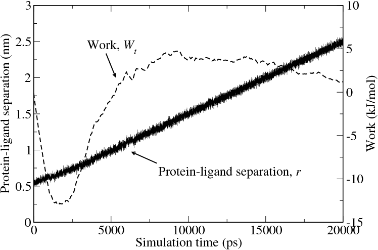
Figure 2: Results shown here are for a single non-equilibrium pulling simulation performed on the FKBP-DMSO system using a pulling speed of $1.0\times 10^{-4}$ nm/ps. The solid line shows the protein-ligand center of mass separation as a function of simulation time. The dashed line shows the accumulated work $W_{t}$ as computed by Eq. (8) as a function of simulation time.

The non-equilibrium unbinding simulations provided us with the protein ligand separation $r$ at every time step, which we used to compute the work and thus the resulting PMF. An example of this is shown in Fig. 2 where we have used Eq. (8) to compute the work as a function of simulation time $W_{t}$.

III.2 Computing $\Delta G^{\text{holo}}_{a}$

We used the Bennett acceptance ratio approach to compute the free energy differences $\Delta G^{\text{holo}}_{a}$ associated with the axial restraints Bennett (1976). With the ligand bound to the protein we performed 1.0 ns equilibrium simulations for each of the values $k_{a}=0,25,40,60,90,150,200,300,450,700,1000$. The first 0.5 ns of each simulation were discarded for equilibration, and the remaining 0.5 ns were used to compute $\Delta G^{\text{holo}}_{a}$. We did not attempt to optimize efficiency of the $\Delta G^{\text{holo}}_{a}$ computations, our only concern was accurate values, so it may be possible to reduce the total computational time from that described above.

III.3 Uncertainty estimation

We estimated the uncertainty in our $\Delta G_{\text{bind}}$ estimates using the bootstrap approach applied to the PMF: (i) The reference value of the PMF given by $\mathcal{W}(r_{*})$ was computed via Eq. (11) using $N$ work values chosen at random (with replacement) from a dataset containing $N$ values; (ii) The above step was repeated until the mean and standard deviation of the free energy estimates converged; around 100,000 trials in our study. (iii) The uncertainty is given by the converged standard deviation of the free energy estimates.

For comparison, we also used the uncertainty analysis obtained by Zuckerman and Woolf Zuckerman and Woolf (2002), and the Bustamante group Gore et al. (2003). These uncertainty estimates are reported to be accurate when the variance in the estimate dominates over the bias (as in the case of large $N$).

III.4 Generating a target PMF

Since the purpose of the current study was to test the effectiveness of non-equilibrium strategies it is important to have an independent estimate of the PMF. Thus, we computed the PMF using umbrella sampling and weighted histogram analysis (WHAM) Kumar et al. (1992). Simulations were performed with the restraints $U_{\text{a}}$ and $U_{\text{r}}$. For the umbrella sampling simulations the speed was set to $v=0$, all other parameters were identical to the non-equilibrium simulations, and 41 windows were used $r_{0}=0.50,0.55,0.60,...,2.45,2.50$. Each window was simulated for a total time of 12 ns; 6 ns were discarded for equilibration and 6 ns were used for the WHAM analysis. Thus, the total simulation time was nearly three times greater than the non-equilibrium simulations detailed above. No attempt was made to test the efficiency since the goal was to generate the most accurate PMF. Note that the $2\ln(r)$ Jacobian correction from Eqs. (7) and (11) were also used for the target PMF.

IV Results and Discussion

The results of this study are very encouraging. Using the non-equilibrium methodology outlined above we estimated the the binding affinity for the FKBP-DMSO and FKBP-BUQ complexes typically within less than 4.0 kJ/mol of the target values; and the target values are within less than 1.0 kJ/mol of experiment.

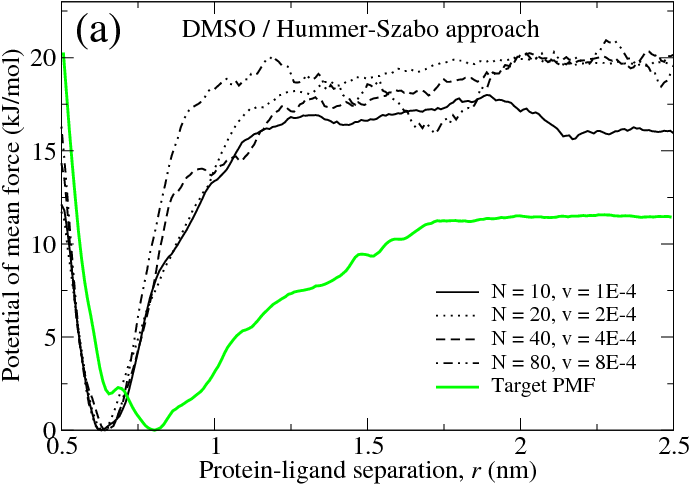
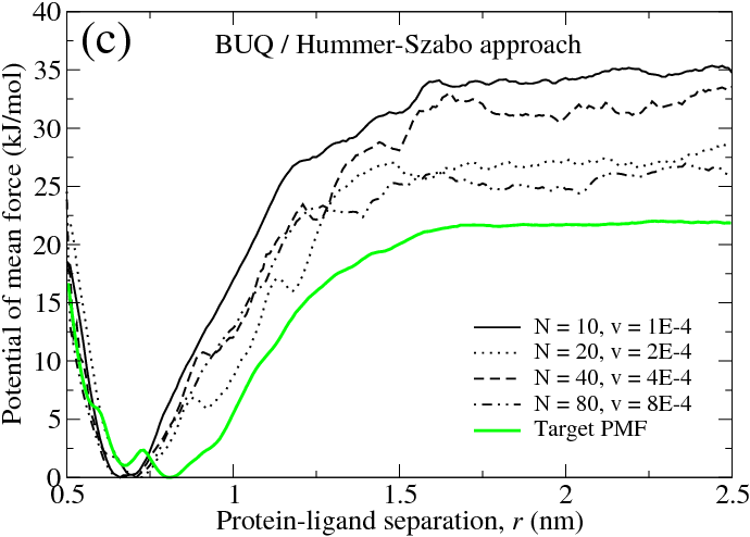
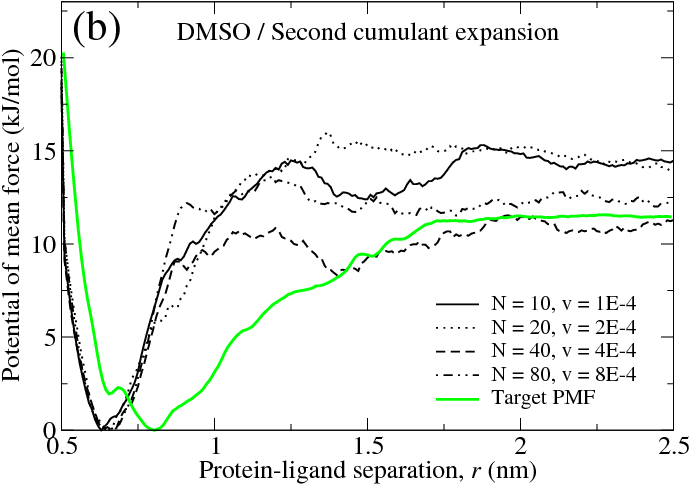
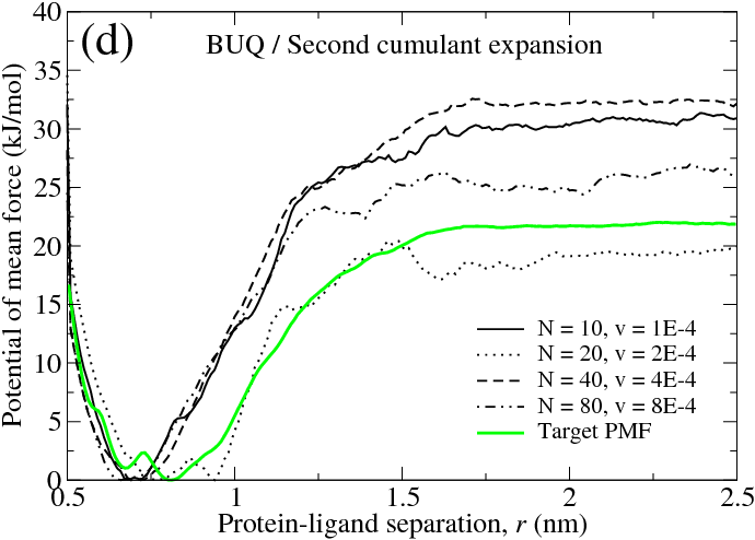
Figure 3: (color online) The PMF as a function of the protein-ligand center of mass separation. These PMF curves were numerically integrated for Eq. (6) and used to generated the $\Delta G_{\text{bind}}$ estimates shown in Table 1. All non-equilibrium results utilized the same total amount of simulation time. For all plots the light colored solid curve shows the target PMF generated via equilibrium umbrella sampling and WHAM. The target PMF curves utilized three times more simulation time as the non-equilibrium simulations, and thus we are not attempting to compare the accuracy of equilibrium and non-equilibrium approaches. (a) FKBP-DMSO system using the Hummer-Szabo approach of Eq. (7). (b) FKBP-DMSO system using the stiff-spring second cumulant expansion approximation of Eq. (11). (c) FKBP-BUQ system using the Hummer-Szabo approach of Eq. (7). (d) FKBP-BUQ system using the stiff-spring second cumulant expansion approximation of Eq. (11).

Figure 3 shows the PMF as a function of protein-ligand separation for all systems studied here. Data is shown for both DMSO and BUQ systems, with pulling speeds indicated on each plot. Note that the same amount of total simulation time was spent on each non-equilibrium PMF estimate, but that the target PMF utilized three times as much simulation as the non-equilibrium estimates, thus we are not attempting to compare non-equilibrium and equilibrium approaches in this study. For both systems the non-equilibrium estimates tend to overestimate the target PMF, and underestimate the broadness of the PMF minimum. This suggests that the pulling speeds were not slow enough to properly sample the PMF. Also, use of stiff-spring approximation with the second cumulant expansion does tend to improve the non-equilibrium PMF curves.

Ligand	$N$	Speed (nm/ps)	$\sigma_{W}$	$\Delta G_{\text{bind}}$a	$\Delta G_{\text{bind}}$b	Unctyc	Unctyd	Targete	Exp
DMSO	10	$1.0\times 10^{-4}$	6.9	-12.6	-11.1	3.5	2.4	-9.2	-9.7
	20	$2.0\times 10^{-4}$	7.9	-15.6	-10.7	1.2	1.0
	40	$4.0\times 10^{-4}$	9.4	-16.3	-8.2	1.6	1.5
	80	$8.0\times 10^{-4}$	10.4	-15.9	-9.2	2.2	1.7
BUQ	10	$1.0\times 10^{-4}$	7.8	-30.0	-26.7	3.1	2.2	-18.3	-18.9
	20	$2.0\times 10^{-4}$	11.9	-23.2	-16.0	4.7	2.4
	40	$4.0\times 10^{-4}$	8.1	-28.4	-28.2	3.8	2.4
	80	$8.0\times 10^{-4}$	11.3	-36.0	-22.3	1.7	1.5

Table 1: Comparison between non-equilibrium binding affinity estimates and target and experimental binding affinities. All energy values are shown in units of kJ/mol. The first column describes the ligand used. The second column contains the number of work values $N$ used in the estimate, and the third and fourth columns are respectively, the corresponding speed of the restraint attached to the ligand, and the standard deviation of the work values. The rightmost column gives the experimental results reported in Ref. Burkhard et al., 2000.
^a Binding affinity estimate obtained via the Hummer-Szabo approach using Eqs. (6) and (7).
^b Binding affinity estimate obtained using the stiff-spring second cumulant expansion approximation using Eqs. (6) and (11).
^c Uncertainty estimate computed via the bootstrap method.
^d Uncertainty estimate computed from the approach described in Refs. Zuckerman and Woolf, 2002; Gore et al., 2003.

Table 1 shows the binding affinity results obtained via Eq. (6), with the PMF computed using both the Hummer-Szabo approach of Eq. (7) and the stiff-spring second cumulant approximation of Eq. (11). The computational estimates of $\Delta G_{\text{bind}}$ for the target PMF are in excellent agreement with experimental data. The non-equilibrium estimates are typically within less than 4.0 kJ/mol of the target values. Reference distances were chosen as $r_{*}=2.4$ nm for both DMSO and BUQ, and the value of the restraint free energy was found to be $\Delta G^{\text{holo}}_{a}=-9.0$ kJ/mol for FKBP-DMSO and $\Delta G^{\text{holo}}_{a}=-7.8$ kJ/mol for FKBP-BUQ. Finally the value of the apo integral in Eq. (6) was computed analytically to be 10.6 kJ/mol for FKBP-DMSO and 10.7 kJ/mol for FKBP-BUQ. The results show that non-equilibrium estimates for the FKBP-DMSO system are more accurate than the FKBP-BUQ estimates suggesting that the FKBP-BUQ system requires more simulation time to converge. Uncertainty estimates were obtained using both a bootstrap method and the approach described in Refs. Zuckerman and Woolf, 2002; Gore et al., 2003.

Table 1 includes the standard deviation of the work values $\sigma_{W}$ measured at the reference distance $r_{*}=2.4$ nm. Previous studies have suggested that the optimal efficiency for use of the Jarzynski relation is when the speed is slow enough that $\sigma_{W}\approx 1.0\;k_{B}T\approx 2.5$ kJ/mol Hummer (2001); Crooks (2000); Ytreberg et al. (2006). Apparently the speeds attempted for the current study were not slow enough to generate work values with such a small $\sigma_{W}$. We note however, for the current study, the uncertainty does not appear to correlate with $\sigma_{W}$. Future studies will be carried out to determine if there is an optimal pulling speed for these systems.

The results from Tab. 1 suggest that use of the Hummer-Szabo approach, while exact in the limit of infinite sampling, is not feasible for the current study. This is likely due to the fact that the pulling speeds used were too fast to generated work values with $\sigma_{W}\approx 1.0\;k_{B}T$. However, use of the approximate stiff-spring second cumulant expansion, while approximate, does tend to improve the $\Delta G_{\text{bind}}$ estimates. This is consistent with the recent study by Minh and McCammon which determined that when similar speeds are utilized the stiff-spring second cumulant expansion method performed better than the other tested methods Minh and McCammon (2008).

We realize that the use of larger more flexible ligands may lead to difficulties in using the method suggested here. This is due to the large number of possible conformations the ligand may adopt in the apo state; all of which must be sampled adequately to obtain an accurate PMF. However, the method may be modified by including an additional restraint to the RMSD of the ligand, thus restricting the conformational freedom of the ligand. The free energy of release from this RMSD restraint must then be included in the binding affinity estimate Woo and Roux (2005); Wang et al. (2006); Mobley et al. (2007).

IV.1 Note on simulation time

Each non-equilibrium estimate in Table 1 was generated using a total simulation time of 216.0 ns (1.0 ns position restrained + 4.0 ns equilibrium to generate starting configurations + 200.0 ns for unbinding simulations + 11.0 ns for $\Delta G^{\text{holo}}_{a}$ estimation). Note however, that the unbinding simulations were performed in parallel. So, for example, at a speed of $2.0\times 10^{-4}$ nm/ps, twenty independent 10.0 ns simulations were performed in parallel. Therefore, all the simulation data needed to compute $\Delta G_{\text{bind}}$ can can be obtained in around a day of wall-clock time with the use of a computer cluster.

V Conclusions

We have demonstrated that non-equilibrium unbinding simulations utilizing a physical pathway can be used to generate estimates of the binding affinity for the FKBP-DMSO and FKBP-BUQ systems studied here. The non-equilibrium estimates are typically within less than 4.0 kJ/mol of the target values; and the target values are within less than 1.0 kJ/mol of experiment.

Our results suggest that when the standard deviation of the work values is larger than the optimal $\sigma_{W}\approx 1.0\;k_{B}T$ that the stiff-spring second cumulant expansion approximation provides a better $\Delta G_{\text{bind}}$ estimate than the exact Hummer-Szabo method.

The importance of pursuing methods such as described here is that such non-equilibrium approaches are trivially parallelizeable since each unbinding simulation is performed independently. Also, due to the use of a physical pathway, the method is simple to implement in many existing simulation packages with little or no modification to the software.

We note that the method described here is not expected to produce accurate binding affinities when the ligand is large and flexible. In this case, it is necessary to extend the approach to include additional restraints to the ligand during the unbinding simulation to prevent large-scale fluctuations. The contribution to the binding affinity from these additional restraints must then be taken into account Woo and Roux (2005); Wang et al. (2006); Mobley et al. (2007).

The results obtained here suggest that non-equilibrium unbinding simulations can be used to generate accurate estimates of binding affinities. Efficiency analysis and comparison to other methodologies will be carried out in future work.

References

- Chipot and Pohorille (2007) C. Chipot and A. Pohorille, Free Energy Calculations: Theory and Applications in Chemistry and Biology (Springer, Berlin, 2007).
- Bash et al. (1987) P. A. Bash, U. C. Singh, F. K. Brown, R. Langridge, and P. A. Kollman, Science 235, 574 (1987).
- Hermans and Wang (1997) J. Hermans and L. Wang, J. Am. Chem. Soc. 119, 2707 (1997).
- Gilson et al. (1997) M. K. Gilson, J. A. Given, B. L. Bush, and J. A. McCammon, Biophys. J. 72, 1047 (1997).
- Chen et al. (2004) W. Chen, C.-E. Chang, and M. K. Gilson, Biophys. J. 87, 3035 (2004).
- Helms and Wade (1998) V. Helms and R. C. Wade, J. Am. Chem. Soc. 120, 2710 (1998).
- Oostenbrink et al. (2000) B. C. Oostenbrink, J. W. Pitera, M. M. van Lipzip, J. H. N. Meerman, and W. F. van Gunsteren, J. Med. Chem. 43, 4594 (2000).
- Dixit and Chipot (2001) S. B. Dixit and C. Chipot, J. Phys. Chem. A 105, 9795 (2001).
- Banavali et al. (2002) N. K. Banavali, W. Im, and B. Roux, J. Chem. Phys. 117, 7381 (2002).
- Boresch et al. (2003) S. Boresch, F. Tettinger, M. Leitgeb, and M. Karplus, J. Phys. Chem. B 107, 9535 (2003).
- Oostenbrink and van Gunsteren (2003) C. Oostenbrink and W. F. van Gunsteren, J. Comput. Chem. 24, 1730 (2003).
- Swanson et al. (2004) J. M. J. Swanson, R. H. Henchman, and J. A. McCammon, Biophys. J. 86, 67 (2004).
- Fujitani et al. (2005) H. Fujitani, Y. Tanida, M. Ito, G. Jayachandran, C. D. Snow, M. R. Shirts, E. J. Sorin, and V. S. Pande, J. Chem. Phys. 123, 084108 (2005).
- Pearlman (2005) D. A. Pearlman, J. Med. Chem. 48, 7796 (2005).
- Carlsson and Aqvist (2005) J. Carlsson and J. Aqvist, J. Phys. Chem. B 109, 6448 (2005).
- Woo and Roux (2005) H.-J. Woo and B. Roux, Proc. Natl. Acad. Sci. USA 102, 6825 (2005).
- Deng and Roux (2006) Y. Deng and B. Roux, J. Chem. Threory Comput. 2, 1255 (2006).
- Wang et al. (2006) J. Wang, Y. Deng, and B. Roux, Biophys. J. 91, 2798 (2006).
- Mobley et al. (2006) D. L. Mobley, J. D. Chodera, and K. A. Dill, J. Chem. Phys. 125, 084902 (2006).
- Jayachandran et al. (2006) G. Jayachandran, M. R. Shirts, S. Park, and V. S. Pande, J. Chem. Phys. 125, 084910 (2006).
- Lee and Olson (2006) M. S. Lee and M. A. Olson, Biophys. J. 90, 864 (2006).
- Mobley et al. (2007) D. L. Mobley, J. D. Chodera, and K. A. Dill, J. Chem. Theory. Comput. 3, 1231 (2007).
- Lee and Olson (2008) M. S. Lee and M. A. Olson, J. Phys. Chem. B 112, 13411 (2008).
- Kirkwood (1935) J. G. Kirkwood, J. Chem. Phys. 3, 300 (1935).
- Zwanzig (1954) R. W. Zwanzig, J. Chem. Phys. 22, 1420 (1954).
- Valleau and Card (1972) J. P. Valleau and D. N. Card, J. Chem. Phys. 57, 5457 (1972).
- Kumar et al. (1992) S. Kumar, J. M. Rosenberg, D. Bouzida, R. H. Swendsen, and P. A. Kollman, J. Comput. Chem. 13, 1011 (1992).
- Jarzynski (1997a) C. Jarzynski, Phys. Rev. Lett. 78, 2690 (1997a).
- Zhang et al. (2006) D. Zhang, J. Gullingsrud, and J. A. McCammon, J. Am. Chem. Soc. 128, 3019 (2006).
- Vashisth and Abrams (2008) H. Vashisth and C. F. Abrams, Biophys. J. 95, 4193 (2008).
- Gräter et al. (2006) F. Gräter, B. L. de Groot, H. Jiang, and H. Grubmüller, Structure 14, 1567 (2006).
- Cuendet and Michielin (2008) M. A. Cuendet and O. Michielin, Biophys. J. 95, 3575 (2008).
- Bastug et al. (2008) T. Bastug, P.-C. Chen, S. M. Patra, and S. Kuyucak, J. Chem. Phys. 128, 155104 (2008).
- Burkhard et al. (2000) P. Burkhard, P. Taylor, and M. D. Walkinshaw, J. Mol. Biol. 295, 953 (2000).
- Van Der Spoel et al. (2005) D. Van Der Spoel, E. Lindahl, B. Hess, G. Groenhof, A. E. Mark, and H. J. C. Berendsen, J. Comput. Chem. 26, 1701 (2005).
- Radmer and Kollman (1997) R. J. Radmer and P. A. Kollman, J. Comput. Chem. 18, 902 (1997).
- Kofke and Cummings (1997) D. A. Kofke and P. T. Cummings, Molec. Phys. 92, 973 (1997).
- Hummer (2001) G. Hummer, J. Chem. Phys. 114, 7330 (2001).
- Shirts and Pande (2005) M. R. Shirts and V. S. Pande, J. Chem. Phys. 122, 144107 (2005).
- Oostenbrink and van Gunsteren (2006) C. Oostenbrink and W. F. van Gunsteren, Chem. Phys. 323, 102 (2006).
- Ytreberg et al. (2006) F. M. Ytreberg, R. H. Swendsen, and D. M. Zuckerman, J. Chem. Phys. 125, 184114 (2006).
- Bennett (1976) C. H. Bennett, J. Comput. Phys. 22, 245 (1976).
- Hummer and Szabo (2001) G. Hummer and A. Szabo, Proc. Natl. Acad. Sci. USA 98, 3658 (2001).
- Hummer and Szabo (2005) G. Hummer and A. Szabo, Acc. Chem. Res. 38, 504 (2005).
- Trzesnial et al. (2007) D. Trzesnial, A.-P. E. Kunz, and W. F. van Gunsteren, Chem. Phys. Chem. 8, 162 (2007).
- Jarzynski (1997b) C. Jarzynski, Phys. Rev. E 56, 5018 (1997b).
- Crooks (2000) G. E. Crooks, Phys. Rev. E 61, 2361 (2000).
- Park et al. (2003) S. Park, F. Khalili-Araghi, E. Tajkhorshid, and K. Schulten, J. Chem. Phys. 119, 3559 (2003).
- Park and Schulten (2004) S. Park and K. Schulten, J. Chem. Phys. 120, 5946 (2004).
- Lu et al. (2003) N. Lu, J. K. Singh, and D. A. Kofke, J. Chem. Phys. 118, 2977 (2003).
- Shirts et al. (2003) M. R. Shirts, E. Bair, G. Hooker, and V. S. Pande, Phys. Rev. Lett. 91, 140601 (2003).
- Lu et al. (2004a) N. Lu, D. A. Kofke, and T. B. Woolf, J. Comput. Chem. 25, 28 (2004a).
- Lu et al. (2004b) N. Lu, D. Wu, T. B. Woolf, and D. A. Kofke, Phys. Rev. E 69, 057702 (2004b).
- Minh and Adib (2008) D. D. L. Minh and A. B. Adib, Phys. Rev. Lett. 100, 180602 (2008).
- Gore et al. (2003) J. Gore, J. Ritort, and C. Bustamante, Proc. Natl. Acad. Sci. USA 100, 12564 (2003).
- Berman et al. (2000) H. M. Berman, J. Westbrook, Z. Feng, G. Gilliland, T. N. Bhat, H. Weissig, I. N. Shindyalov, and P. E. Bourne, Nucl. Acids Res. 28, 235 (2000).
- Schuettelkopf and van Aalten (2004) A. W. Schuettelkopf and D. M. F. van Aalten, Acta Cryst. D 60, 1355 (2004).
- van Gunsteren et al. (1996) W. F. van Gunsteren, S. R. Billeter, A. A. Eising, P. H. Hünenberger, P. Krüger, A. E. Mark, W. R. P. Scott, and I. G. Tironi, Biomolecular Simulation: The GROMOS96 manual and user guide (Hochschulverlag, Zürich, 1996).
- Berendsen et al. (1981) H. J. C. Berendsen, J. P. M. Postma, W. F. van Gunsteren, and J. Hermans, Intermolecular Forces (Reidel, Dordrecht, 1981).
- van Gunsteren et al. (1981) W. F. van Gunsteren, H. J. C. Berendsen, and J. A. C. Rullmann, Mol. Phys. 44, 69 (1981).
- Berendsen et al. (1984) H. J. C. Berendsen, J. P. M. Postma, W. F. van Gunsteren, A. DiNola, and J. R. Haak, J. Chem. Phys. 81, 3684 (1984).
- Hess et al. (1997) B. Hess, H. Bekker, H. J. C. Berendsen, and J. G. E. M. Fraaije, J. Comput. Chem. 18, 1463 (1997).
- Darden et al. (1993) T. Darden, D. York, and L. Pedersen, J. Chem. Phys. 98, 10089 (1993).
- Allen and Tildesley (1989) M. P. Allen and D. J. Tildesley, Computer Simulation of Liquids (Oxford University Press, New York, 1989).
- Zuckerman and Woolf (2002) D. M. Zuckerman and T. B. Woolf, Phys. Rev. Lett. 89, 180602 (2002).
- Minh and McCammon (2008) D. D. L. Minh and J. A. McCammon, J. Phys. Chem. B 112, 5892 (2008).