Weak measurement takes a simple form for cumulants

Abstract

A weak measurement on a system is made by coupling a pointer weakly to the system and then measuring the position of the pointer. If the initial wavefunction for the pointer is real, the mean displacement of the pointer is proportional to the so-called weak value of the observable being measured. This gives an intuitively direct way of understanding weak measurement. However, if the initial pointer wavefunction takes complex values, the relationship between pointer displacement and weak value is not quite so simple, as pointed out recently by R. Jozsa Jozsa (2007). This is even more striking in the case of sequential weak measurements Mitchison et al. (2007). These are carried out by coupling several pointers at different stages of evolution of the system, and the relationship between the products of the measured pointer positions and the sequential weak values can become extremely complicated for an arbitrary initial pointer wavefunction. Surprisingly, all this complication vanishes when one calculates the cumulants of pointer positions. These are directly proportional to the cumulants of sequential weak values. This suggests that cumulants have a fundamental physical significance for weak measurement.

I Introduction

In physics, formal simplicity is often a reliable guide to the significance of a result. The concept of weak measurement, due to Aharonov and his coworkers Aharonov and Rohrlich (2005); Aharonov et al. (1988), derives some of its appeal from the formal simplicity of its basic formulae. One can extend the basic concept to a sequence of weak measurements carried out at a succession of points during the evolution of a system Mitchison et al. (2007), but then the formula relating pointer positions to weak values turns out to be not quite so simple, particularly if one allows arbitrary initial conditions for the measuring system. I show here that the complications largely disappear if one takes the cumulants of expected values of pointer positions; these are related in a formally satisfying way to weak values, and this form is preserved under all measurement conditions.

The goal of weak measurement is to obtain information about a quantum system given both an initial state $|\psi_{i}\rangle$ and a final, post-selected state $|\psi_{f}\rangle$. Since weak measurement causes only a small disturbance to the system, the measurement result can reflect both the initial and final states. It can therefore give richer information than a conventional (strong) measurement, including in particular the results of all possible strong measurements Oreshkov and A.Brun (2005); Bennett et al. (1999). To carry out the measurement, a measuring device is coupled to the system in such a way that the system is only slightly perturbed; this can be achieved by having a small coupling constant $g$. After the interaction, the pointer’s position $q$ is measured (or possibly some other pointer observable; e.g. its momentum $p$). Suppose that, following the standard von Neumann paradigm, von Neumann (1955), the interaction between measuring device and system is taken to be $H_{int}=g\delta(t)pA$, where $p$ is the momentum of a pointer and the delta function indicates an impulsive interaction at time $t$. It can be shown Aharonov et al. (1988) that the expectation of the pointer position, ignoring terms of order $g^{2}$ or higher, is

$$\langle q\rangle=gReA_{w},$$ (1)

where $A_{w}$ is the weak value of the observable $A$ given by

$$A_{w}=\frac{\langle\psi_{f}|A|\psi_{i}\rangle}{\langle\psi_{f}|\psi_{i}\rangle}.$$ (2)

As can be seen, (1) has an appealing simplicity, relating the pointer shift directly to the weak value. However, this formula only holds under the rather special assumption that the initial pointer wavefunction $\phi$ is a gaussian, or, more generally, is real and has zero mean. When $\phi$ is a completely general wavefunction, i.e. is allowed to take complex values and have any mean value Jozsa (2007); Mitchison et al. (2007), equation (1) is replaced by

$$\langle q\rangle=\langle q\rangle_{i}+gReA_{w}+gImA_{w}\left(\langle pq+qp\rangle_{i}-2\langle q\rangle_{i}\langle p\rangle_{i}\right),$$ (3)

where, for any pointer variable $x$, $\langle x\rangle_{i}$ denotes the initial expected value $\langle\phi|x|\phi\rangle$ of $x$; so for instance $\langle q\rangle_{i}$ and $\langle p\rangle_{i}$ are the means of the initial pointer position and momentum, respectively. (Again, this formula ignores terms of order $g^{2}$ or higher.)

Equation (3) seems to have lost the simplicity of (1), but we can rewrite it as

$$\langle q\rangle=\langle q\rangle_{i}+gRe(\xi A_{w}),$$ (4)

where

$$\xi=-2i\left(\langle qp\rangle_{i}-\langle q\rangle_{i}\langle p\rangle_{i}\right),$$ (5)

and equation (4) is then closer to the form of (1). As will become clear, this is part of a general pattern.

One can also weakly measure several observables, $A_{1},\ldots,A_{n}$, in succession Mitchison et al. (2007). Here one couples pointers at several locations and times during the evolution of the system, taking the coupling constant $g_{k}$ at site $k$ to be small. One then measures each pointer, and takes the product of the positions $q_{k}$ of the pointers. For two observables, and in the special case where the initial pointer distributions are real and have zero mean, e.g. a gaussian, one finds Mitchison et al. (2007)

$$\langle q_{1}q_{2}\rangle=\frac{g_{1}g_{2}}{2}\ Re\left[(A_{2},A_{1})_{w}+(A_{1})_{w}\overline{(A_{2})}_{w}\right],$$ (6)

ignoring terms in higher powers of $g_{1}$ and $g_{2}$. Here $(A_{2},A_{1})_{w}$ is the sequential weak value defined by

$$(A_{2},A_{1})_{w}=\frac{\langle\psi_{f}|WA_{2}VA_{1}U|\psi_{i}\rangle}{\langle\psi_{f}|WVU|\psi_{i}\rangle},$$ (7)

where $U$ is a unitary taking the system from the initial state $|\psi_{i}\rangle$ to the first weak measurement, $V$ describes the evolution between the two measurements, and $W$ takes the system to the final state. (Note the reverse order of operators in $(A_{2},A_{1})$, which reflects the order in which they are applied.) If we drop the assumption about the special initial form of the pointer distribution and allow an arbitrary $\phi$, then the counterpart of (6) becomes extremely complicated: see Appendix, equation 72.

Even the comparatively simple formula (6) is not quite ideal. By analogy with (1) we would hope for a formula of the form $\langle q_{1}q_{2}\rangle\propto Re(A_{2},A_{1})_{w}$, but there is an extra term $(A_{1})_{w}\overline{(A_{2})}_{w}$. What we seek, therefore, is a relationship that has some of the formal simplicity of (1) and furthermore preserves its form for all measurement conditions. It turns out that this is possible if we take the cumulant of the expectations of pointer positions. As we shall see in the next section, this is a certain sum of products of joint expectations of subsets of the $q_{i}$, which we denote by $\langle q_{1}\ldots q_{n}\rangle^{c}$. For a set of observables, we can define a formally equivalent expression using sequential weak values, which we denote by $(A_{n},\ldots,A_{1})^{c}_{w}$. Then the claim is that, up to order $n$ in the coupling constants $g_{k}$ (assumed to be all of the same approximate order of magnitude):

$$\langle q_{1}\ldots q_{n}\rangle^{c}=g_{1}\ldots g_{n}Re\left\{\xi(A_{n},\ldots,A_{1})_{w}^{c}\right\},$$ (8)

where $\xi$ is a factor dependent on the initial wavefunctions for each pointer. Equation (8) holds for any initial pointer wavefunction, though different wavefunctions produce different values of $\xi$. The remarkable thing is that all the complexity is packed into this one number, rather than exploding into a multiplicity of terms, as in (72).

Note also that (4) has essentially the same form as (8) since, in the case $n=1$, $\langle A\rangle^{c}_{w}=A_{w}$. However, there is an extra term $\langle q\rangle_{i}$ in (4); this arises because the cumulant for $n=1$ is anomalous in that its terms do not sum to zero.

II Cumulants

Given a collection of random variables, such as the pointer positions $q_{i}$, the cumulant $\langle q_{1}\ldots q_{n}\rangle^{c}$ is a polynomial in the expectations of subsets of these variables Kendall and Stuart (1977); Royer (1983); it has the property that it vanishes whenever the set of variables $q_{i}$ can be divided into two independent subsets. One can say that the cumulant, in a certain sense, picks out the maximal correlation involving all of the variables.

We introduce some notation to define the cumulant. Let $x$ be a subset of the integers $\{1,\ldots,n\}$. We write $\prod_{x}q$ for $\prod_{i=1}^{|x|}q_{x(i)}$, where $|x|$ is the size of $x$ and the indices of the $q$’s in the product run over all the integers $x(i)$ in $x$. Then the cumulant is given by

$$\langle q_{1}\ldots q_{n}\rangle^{c}=\sum_{b=\{b_{1},\ldots,b_{k}\}}a_{k}\prod_{j=1}^{k}\left\langle\prod_{b_{j}}q\right\rangle,$$ (9)

where $b=\{b_{1},\ldots,b_{k}\}$ runs over all partitions of the integers $\{1,\ldots,n\}$ and the coefficient $a_{k}$ is given by

$$a_{k}=(k-1)!(-1)^{k-1}.$$ (10)

For $n=1$ we have $\langle q\rangle^{c}=\langle q\rangle$, and for $n=2$

$$\langle q_{1}q_{2}\rangle^{c}=\langle q_{1}q_{2}\rangle-\langle q_{1}\rangle\langle q_{2}\rangle.$$ (11)

There is an inverse operation for the cumulant Zhou et al. (2006); Royer (1983):

Proposition II.1.

$$\langle q_{1}\ldots q_{n}\rangle=\sum_{b=\{b_{1},\ldots,b_{k}\}}\prod_{j=1}^{k}\left\langle\prod_{b_{j}}q\right\rangle^{c}.$$ (12)

Proof.

To see that this equation holds, we must show that the term $\prod_{j=1}^{k}\langle\prod_{b_{j}}q\rangle$ obtained by expanding the right-hand side is zero unless $b$ is the partition consisting of the single set $\{1,\ldots,n\}$. Replacing each subset $b_{j}$ by the integer $j$, this is equivalent to $\sum a_{k_{1}}\ldots a_{k_{r}}=0$, where the sum is over all partitions of $\{1,\ldots,k\}$ by subsets of sizes $k_{1},\ldots,k_{r}$ and the $a_{k}$’s are given by (10). In this sum we distinguish partitions with distinct integers; e.g. $\{1,2\},\{3,4\}$ and $\{1,3\},\{2,4\}$. There are $\binom{k}{k_{1}\ldots k_{r}}(l_{1}!\ldots l_{k}!)^{-1}$ such distinct partitions with subset sizes $k_{1}\ldots k_{r}$, where $l_{i}$ is the number of $k$’s equal to $i$, so our sum may be rewritten as $k!\sum(-1)^{k_{1}-1}\ldots(-1)^{k_{r}-1}(l_{1}!\ldots l_{k}!k_{1}\ldots k_{r})^{-1}$, where the sum is now over partitions in the standard sense Apostol (1976). This is $k!$ times the coefficient of $x^{k}$ in

$$\left(1+x+\frac{x^{2}}{2!}+\ldots\right)\left(1+(-x^{2}/2)+\frac{(-x^{2}/2)^{2}}{2!}+\ldots\right)\left(1+(x^{3}/3)+\frac{(x^{3}/3)^{2}}{2!}+\ldots\right)\ldots$$ (13)

$$=e^{x-x^{2}/2+x^{3}/3\ldots}=e^{log_{e}(1+x)}=1+x.$$ (14)

Thus the sum is zero except for $k=1$, which corresponds to the single-set partition $b$. ∎

Definition II.2.

If $\{1,\ldots,n\}$ can be written as the disjoint union of two subsets $S_{1}$ and $S_{2}$, we say the variables corresponding to these subsets are independent if

$$\langle\prod_{S_{1}^{\prime}}q\prod_{S_{2}^{\prime}}q\rangle=\langle\prod_{S_{1}^{\prime}}q\rangle\langle\prod_{S_{2}^{\prime}}q\rangle,$$ (15)

for any subsets $S_{i}^{\prime}\subseteq S_{i}$.

We now prove the characteristic property of cumulants:

Proposition II.3.

The cumulant vanishes if its arguments can be divided into two independent subsets.

Proof.

For $n=2$ this follows at once from (11) and (15), and we continue by induction. From (12) and the inductive assumption for $n-1$, we have

$$\langle q_{1}\ldots q_{n}\rangle=\langle q_{1}\ldots q_{n}\rangle^{c}+\sum_{b=\{b_{1},\ldots,b_{k}\}\subset S_{1}}\prod_{j=1}^{k}\left\langle\prod_{b_{j}}q\right\rangle^{c}\sum_{c=\{c_{1},\ldots,c_{l}\}\subset S_{2}}\prod_{j=1}^{l}\left\langle\prod_{c_{j}}q\right\rangle^{c}.$$ (16)

This holds because any term on the right-hand side of (12) vanishes when any subset of the partition $b$ includes elements of both $S_{1}$ and $S_{2}$. Using (12) again, this implies

$$\langle q_{1}\ldots q_{n}\rangle=\langle q_{1}\ldots q_{n}\rangle^{c}+\langle\prod_{S_{1}}q\rangle\langle\prod_{S_{2}}q\rangle,$$ (17)

and by independence, $\langle q_{1}\ldots q_{n}\rangle^{c}=0$. Thus the inductive assumption holds for $n$. ∎

In fact, the coefficients $a_{k}$ in (9) are uniquely determined to have the form (10) by the requirement that the cumulant vanishes when the variables form two independent subsets Percus (1975); Simon (1979).

For $n=2$, the cumulant (11) is just the covariance, $\langle q_{1}q_{2}\rangle^{c}=\langle(q_{1}-\langle q_{1}\rangle)(q_{2}-\langle q_{2}\rangle)\rangle$, and the same is true for $n=3$, namely $\langle q_{1}q_{2}q_{3}\rangle^{c}=\langle(q_{1}-\langle q_{1}\rangle)(q_{2}-\langle q_{2}\rangle)(q_{3}-\langle q_{3}\rangle)\rangle$. For $n=4$, however, there is a surprise. The covariance is given by

$$\langle\prod_{i=1}^{4}(q_{i}-\langle q_{i}\rangle)\rangle=\langle q_{1}q_{2}q_{3}q_{4}\rangle-\sum\langle q_{i}q_{j}q_{k}\rangle\langle q_{l}\rangle+\sum\langle q_{i}q_{j}\rangle\langle q_{k}\rangle\langle q_{l}\rangle-3\langle q_{1}\rangle\langle q_{2}\rangle\langle q_{3}\rangle\langle q_{4}\rangle,$$ (18)

where the sums include all distinct combinations of indices, but the cumulant is

$$\langle q_{1}q_{2}q_{3}q_{4}\rangle^{c}=\langle q_{1}q_{2}q_{3}q_{4}\rangle-\sum\langle q_{i}q_{j}q_{k}\rangle\langle q_{l}\rangle-\sum\langle q_{i}q_{j}\rangle\langle q_{k}q_{l}\rangle+2\sum\langle q_{i}q_{j}\rangle\langle q_{k}\rangle\langle q_{l}\rangle-6\langle q_{1}\rangle\langle q_{2}\rangle\langle q_{3}\rangle\langle q_{4}\rangle,$$ (19)

which includes terms like $\langle q_{1}q_{2}\rangle\langle q_{3}q_{4}\rangle$ that do not occur in the covariance. Note that, if the subsets $\{1,2\}$ and $\{3,4\}$ are independent, the covariance does not vanish, since independence implies we can write the first term in (18) as $\langle q_{1}q_{2}q_{3}q_{4}\rangle=\langle q_{1}q_{2}\rangle\langle q_{3}q_{4}\rangle$ and there is no cancelling term. However, as we have seen, the cumulant does contain such a term, and it is a pleasant exercise to check that the whole cumulant vanishes.

III Sequential weak values and cumulants

To carry out a sequential weak measurement, one starts a system in an initial state $|\psi_{i}\rangle$, then weakly couples pointers at several times $t_{k}$ during the evolution of the system, and finally post-selects the system state $|\psi_{f}\rangle$. One then measures the pointers and finally takes the product of the values obtained from these pointer measurements. It is assumed that one can repeat the whole process many times to obtain the expectation of the product of pointer values. If one measures pointer positions $q_{k}$, for instance, one can estimate $\langle q_{1}\ldots q_{n}\rangle$, but one could also measure the momenta of the pointers to estimate $\langle p_{1}\ldots p_{n}\rangle$.

If the coupling for the $k$th pointer is given by $H_{int}=\delta(t-t_{k})r_{k}p$, and if the individual initial pointer wavefunctions are gaussian, or, more generally, are real with zero mean, then it turns out Mitchison et al. (2007) that these expectations can be expressed in terms of sequential weak values of order $n$ or less. Here the sequential weak value of order $n$, $(A_{n},\ldots A_{1})_{w}$, is defined by

$$(A_{n},\ldots A_{1})_{w}=\frac{\langle\psi_{f}|U_{n+1}A_{n}U_{n}\ldots A_{1}U_{1}|\psi_{i}\rangle}{\langle\psi_{f}|U_{n+1}\ldots U_{1}|\psi_{i}\rangle},$$ (20)

where $U_{i}$ defines the evolution of the system between the measurements of $A_{i-1}$ and $A_{i}$.

When the $A_{k}$ are projectors, $A_{k}=|x_{k}\rangle\langle x_{k}|$, we can write the sequential weak value as Mitchison et al. (2007)

$$(A_{n},\ldots A_{1})_{w}=\frac{\langle\psi_{f}|U_{n+1}|x_{n}\rangle\ \langle x_{n}|U_{n}|x_{n-1}\rangle\ldots\langle x_{1}|U_{1}|\psi_{i}\rangle}{\sum_{y}\langle\psi_{f}|U_{n+1}|y_{n}\rangle\ \langle y_{n}|U_{n}|y_{n-1}\rangle\ldots\langle y_{1}|U_{1}|\psi_{i}\rangle}=\frac{\mbox{amplitude}(x)}{\sum_{y}\mbox{amplitude}(y)},$$ (21)

which shows that, in this case, the weak values has a natural interpretation as the amplitude for following the path defined by the $x_{k}$. Figure 9 shows an example taken from Mitchison et al. (2007) where the path (labelled by ’1’ and ’2’ successively) is a route taken by a photon through a pair of interferometers, starting by injecting the photon at the top left (with state $|\psi\rangle_{i}$) and ending with post-selection by detection at the bottom right (with final state $|\psi\rangle_{f}$).

Figure 1:

In the last section, the cumulant was defined for expectations of products of variables. One can define the cumulant for other entities by formal analogy; for instance for density matrices Zhou et al. (2006), or hypergraphs Royer (1983). We can do the same for sequential weak values, defining the cumulant by (9) with $\langle\prod_{b_{j}}q\rangle$ replaced by $(\overleftarrow{A_{b_{j}(|b_{j}|)},\ldots A_{b_{j}(1)}})_{w}$, where the arrow indicates that the indices, which run over the subset $b_{j}$, are arranged in ascending order from right to left. For example, for $n=1$, $(A_{w})^{c}=A_{w}$, and for $n=4$

$$(A_{4},A_{3},A_{2},A_{1})^{c}_{w} =(A_{4},A_{3},A_{2},A_{1})_{w}-\sum(\overleftarrow{A_{i},A_{j},A_{k}})_{w}(A_{l})_{w}-\sum(\overleftarrow{A_{i},A_{j}})_{w}(\overleftarrow{A_{k},A_{l}})_{w}$$ (22)

$$+2\sum(\overleftarrow{A_{i},A_{j}})_{w}(A_{k})_{w}(A_{l})_{w}-6(A_{1})_{w}(A_{2})_{w}(A_{3})_{w}(A_{4})_{w}.$$

There is a notion of independence that parallels (15): given a disjoint partition $S_{1}\cup S_{2}=\{1,\ldots,n\}$ such that

$$(\overleftarrow{A_{S_{1}^{\prime}\cup S_{2}^{\prime}}})_{w}=(\overleftarrow{A_{S_{1}^{\prime}}})_{w}(\overleftarrow{A_{S_{2}^{\prime}}})_{w},$$ (23)

for any subsets $S_{i}^{\prime}\subseteq S_{i}$, then we say the observables labelled by the two subsets are weakly independent. There is then an analogue of Lemma II.3:

Lemma III.1.

The cumulant $(A_{n},\ldots,A_{1})_{w}^{c}$ vanishes if the $A_{k}$ are weakly independent for some subsets $S_{1}$, $S_{2}$.

As an example of this, if one is given a bipartite system $\mathcal{H}^{A}\otimes\mathcal{H}^{B}$, and initial and final states that factorise as $|\psi_{i}\rangle=|\psi_{i}\rangle^{A}\otimes|\psi_{i}\rangle^{B}$ and $|\psi_{f}\rangle=|\psi_{f}\rangle^{A}\otimes|\psi_{f}\rangle^{B}$, then observables on the $A$- and $B$-parts of the system are clearly weakly independent. Another class of examples comes from what one might describe as a “bottleneck” construction, where, at some point the evolution of the system is divided into two parts by a one-dimensional projector (the bottleneck) and its complement, and the post-selection excludes the complementary part. Then, if all the measurements before the projector belong to $S_{1}$ and all those after the projector belong to $S_{2}$, the two sets are weakly independent. This follows because we can write

$$(\overleftarrow{A_{S_{1}^{\prime}\cup S_{2}^{\prime}}})_{w} =\frac{\langle\psi_{f}|U_{n+1}A_{n}\ldots U_{k+1}A_{k}W_{k}|\psi_{b}\rangle\langle\psi_{b}|V_{k}A_{k-1}\ldots A_{1}U_{1}|\psi_{i}\rangle}{\langle\psi_{f}|U_{n+1}\ldots U_{k+1}W_{k}|\psi_{b}\rangle\langle\psi_{b}|V_{k}\ldots U_{1}|\psi_{i}\rangle}$$

$$=\frac{\langle\psi_{f}|U_{n+1}A_{n}\ldots U_{k+1}A_{k}W_{k}|\psi_{b}\rangle\langle\psi_{b}|V_{k}\ldots U_{1}|\psi_{i}\rangle}{\langle\psi_{f}|U_{n+1}\ldots U_{k+1}W_{k}|\psi_{b}\rangle\langle\psi_{b}|V_{k}\ldots U_{1}|\psi_{i}\rangle}\ \ \frac{\langle\psi_{f}|U_{n+1}\ldots U_{k+1}W_{k}|\psi_{b}\rangle\langle\psi_{b}|V_{k}A_{k-1}\ldots A_{1}U_{1}|\psi_{i}\rangle}{\langle\psi_{f}|U_{n+1}\ldots U_{k+1}W_{k}|\psi_{b}\rangle\langle\psi_{b}|V_{k}\ldots U_{1}|\psi_{i}\rangle}$$

$$=(\overleftarrow{A_{S_{1}^{\prime}}})_{w}(\overleftarrow{A_{S_{2}^{\prime}}})_{w},$$

where $W_{k}|\psi_{b}\rangle\langle\psi_{b}|V_{k}$ is the part of $U_{k}$ lying in the post-selected subspace. As an illustration of this, suppose we add a connecting link (Figure 2, “$L$”) between the two interferometers in Figure 1, so $|\psi_{b}\rangle\langle\psi_{b}|$, the bottleneck, is the projection onto $L$, and post-selection discards the part of the wavefunction corresponding to the path $L^{\prime}$. Then measurements at ‘1’ and ‘2’ are weakly independent; in fact $(A_{1})_{w}=1/2$, $(A_{2})_{w}=1/2$ and $(A_{2},A_{1})_{w}=1/4$. Note that the same measurements are not independent in the double interferometer of Figure 1, where $(A_{1})_{w}=0$, $(A_{2})_{w}=0$, and yet, surprisingly, $(A_{2},A_{1})_{w}=-1/2$, Mitchison et al. (2007).

Figure 2:

IV The main theorem

Consider $n$ system observables $A_{1},\ldots,A_{n}$. Suppose $s_{k}$, for $k=1,\dots,n$, are observables of the $k$th pointer, namely Hermitian functions $s_{k}(q_{k},p_{k})$ of pointer position $q_{k}$ and momentum $p_{k}$, and the interaction Hamiltonian for the weak measurement of system observable $A_{k}$ is $H_{k}=g_{k}s_{k}A_{k}$, where $g_{k}$ is a small coupling constant (all $g_{k}$ being assumed of the same order of magnitude $g$). Suppose further that the pointer observables $r_{k}$ are measured after the coupling. Let $\phi_{k}$ be the $k$-th pointer’s initial wave-function. For any variable $x_{k}$ associated to the $k$-th pointer, write $\langle x_{k}\rangle_{i}$ for $\langle\phi_{k}|x_{k}|\phi_{k}\rangle$.

We are now almost ready to state the main theorem, but first need to clarify the measurement procedure. When we evaluate expectations of products of the $r_{k}$ for different sets of pointers, for instance when we evaluate $\langle r_{1}r_{2}\rangle$, we have a choice. We could either couple the entire set of $n$ pointers and then select the data for pointers 1 and 2 to get $\langle r_{1}r_{2}\rangle$. Or we could carry out an experiment in which we couple just pointers 1 and 2 to give $\langle r_{1}r_{2}\rangle$. These procedures give different answers. For instance, if we couple three pointers and measure pointers 1 and 2 to get $\langle r_{1}r_{2}\rangle$, in addition to the terms in $g_{1}$, $g_{2}$ and $g_{1}g_{2}$ we also get terms in $g_{2}g_{3}$ and $g_{1}g_{3}$ involving the observable $A_{3}$. This means we get a different cumulant $\langle r_{1}\ldots r_{n}\rangle^{c}$, depending on the procedure used. In what follows, we regard each expectation as being evaluated in a separate experiment, with only the relevant pointers coupled. It will be shown elsewhere that, with the alternative definition, the theorem still holds but with a different value of the constant $\xi$.

Theorem IV.1 (Cumulant theorem).

For $n\geq 2$, for any pointer observables $r_{k}$ and $s_{k}$, and for any initial pointer wavefunctions $\phi_{k}$, up to total order $n$ in the $g_{k}$,

$$\langle r_{1}\ldots r_{n}\rangle^{c}=g_{1}\ldots g_{n}Re\left\{\xi(A_{n},\ldots,A_{1})^{c}_{w}\right\},$$ (24)

where $\xi$ (sometimes written more explicitly as $\xi_{r_{1}\ldots r_{n}}$) is given by

$$\xi=2(-i)^{n}\left(\prod_{k=1}^{n}\langle r_{k}s_{k}\rangle_{i}-\prod_{k=1}^{n}\langle r_{k}\rangle_{i}\langle s_{k}\rangle_{i}\right).$$ (25)

For $n=1$ the same result holds, but with the extra term $\langle r\rangle_{i}$:

$$\langle r\rangle=\langle r\rangle_{i}+gRe(\xi A_{w}).$$ (26)

Proof.

We use the methods of Mitchison et al. (2007) to calculate the expectations of products of pointer variables for sequential weak measurements. Let the initial and final states of the system be $|\psi_{i}\rangle$ and $|\psi_{f}\rangle$, respectively. Consider some subset $b=\{b_{1},\ldots,b_{\kappa}\}$ of $\{1,\ldots,n\}$, with $b_{1}\leq b_{2}\leq\ldots\leq b_{\kappa}$. The state of the system and the pointers $b_{1},\ldots,b_{\kappa}$ after the coupling of those pointers is

$$\Psi_{\mathcal{S},\mathcal{M}}=U_{n+1}\dots U_{b_{\kappa}+1}e^{-ig_{b_{\kappa}}s_{b_{\kappa}}A_{b_{\kappa}}}U_{b_{\kappa}}\ldots e^{-ig_{b_{1}}s_{b_{1}}A_{b_{1}}}U_{b_{1}}\dots U_{1}|\psi_{i}\rangle\phi_{b_{1}}(r_{b_{1}})\ldots\phi_{b_{\kappa}}(r_{b_{\kappa}}),$$ (27)

and following post-selection by the system state $|\psi_{f}\rangle$, the state of the pointers is

$$\Psi_{\mathcal{M}}=\langle\psi_{f}|U_{n+1}\dots U_{b_{\kappa}+1}e^{-ig_{b_{\kappa}}s_{b_{\kappa}}A_{b_{\kappa}}}U_{b_{\kappa}}\ldots e^{-ig_{b_{1}}s_{b_{1}}A_{b_{1}}}U_{b_{1}}\dots U_{1}|\psi_{i}\rangle\phi_{b_{1}}(r_{b_{1}})\ldots\phi_{b_{\kappa}}(r_{b_{\kappa}}).$$ (28)

Expanding each exponential, we have

$$\langle r_{b_{1}}\ldots r_{b_{\kappa}}\rangle =\frac{\int\overline{\Psi}_{\mathcal{M}}r_{b_{1}}\ldots r_{b_{\kappa}}\Psi_{\mathcal{M}}dr_{b_{1}}\ldots dr_{b_{\kappa}}}{\int|\Psi_{\mathcal{M}}|^{2}dr_{b_{1}}\ldots dr_{b_{\kappa}}},$$ (29)

$$=\frac{\sum_{i_{1}\ldots i_{n}\in b\ ;\ j_{1}\ldots j_{n}\in b}\ \alpha_{i_{1}\ldots i_{n}}\overline{\alpha}_{j_{1}\ldots j_{n}}u^{b_{1}}_{i_{b_{1}}j_{b_{1}}}\ldots u^{b_{\kappa}}_{i_{b_{\kappa}}j_{b_{\kappa}}}}{\sum_{i_{1}\ldots i_{n}\in b\ ;\ j_{1}\ldots j_{n}\in b}\ \alpha_{i_{1}\ldots i_{n}}\overline{\alpha}_{j_{1}\ldots j_{n}}v^{b_{1}}_{i_{b_{1}}j_{b_{1}}}\ldots v^{b_{\kappa}}_{i_{b_{\kappa}}j_{b_{\kappa}}}},$$ (30)

where $i_{k}\geq 0$ are integers, $i_{1},\ldots,i_{n}\in b$ means that $i_{l}=0$ for $l\notin b$, and

$$\alpha_{i_{1}\ldots i_{n}} =\left(\prod_{k=1}^{n}g_{k}^{i_{k}}\right)\ (A^{i_{n}}_{n},\ldots A^{i_{1}}_{1})_{w},$$ (31)

$$u^{k}_{lm} =\int(m!)^{-1}\overline{(-is_{k})^{m}\phi_{k}(r_{k})}r_{k}(l!)^{-1}(-is_{k})^{l}\phi_{k}(r_{k})dr_{k},$$ (32)

$$v^{k}_{lm} =\int(m!)^{-1}\overline{(-is_{k})^{m}\phi_{k}(r_{k})}(l!)^{-1}(-is_{k})^{l}\phi_{k}(r_{k})dr_{k}.$$ (33)

Let us write (30) as

$$\langle r_{b_{1}}\ldots r_{b_{\kappa}}\rangle=\frac{\sum_{{\bf i}\in b,{\bf j}\in b}x_{{\bf i};{\bf j}}}{\sum_{{\bf i}\in b,{\bf j}\in b}y_{{\bf i};{\bf j}}},$$ (34)

where

$$x_{{\bf i};{\bf j}} =\alpha_{i_{1}\ldots i_{n}}\overline{\alpha}_{j_{1}\ldots j_{n}}u^{b_{1}}_{i_{b_{1}}j_{b_{1}}}\ldots u^{b_{\kappa}}_{i_{b_{\kappa}}j_{b_{\kappa}}},$$ (35)

$$y_{{\bf k};{\bf l}} =\alpha_{k_{1}\ldots k_{n}}\overline{\alpha}_{l_{1}\ldots l_{n}}v^{b_{1}}_{i_{b_{1}}j_{b_{1}}}\ldots v^{b_{\kappa}}_{i_{b_{\kappa}}j_{b_{\kappa}}},$$ (36)

and ${\bf i}$ denotes the index set $\{i_{1}\ldots i_{n}\}$, etc.. Define

$$X_{b}=\sum_{{\bf i}\in b,{\bf j}\in b}x_{{\bf i};{\bf j}},\ \ Y_{b}=\sum_{{\bf i}\in b,{\bf j}\in b}y_{{\bf i};{\bf j}}.$$ (37)

Then

$$\langle r_{1},\ldots,r_{n}\rangle^{c} =\sum_{b_{1},\ldots,b_{k}}(k-1)!(-1)^{k-1}\prod_{l=1}^{k}\langle r_{b_{l}(1)}\ldots r_{b_{l}(|b_{l}|)}\rangle$$ (38)

$$=\sum_{b_{1},\ldots,b_{k}}(k-1)!(-1)^{k-1}\prod_{l=1}^{k}\frac{X_{b_{l}}}{Y_{b_{l}}}.$$ (39)

Set $\mathcal{Y}=\prod_{b\subset\{1,\ldots,n\}}Y_{b}$, where $b$ in the product ranges over all distinct subsets of the integers $\{1,\ldots,n\}$. Then $\mathcal{Y}\langle r_{1}\ldots r_{n}\rangle^{c}$ is an (infinite) weighted sum of terms

$$z_{\mathcal{I}}=(x_{{\bf i}(1);{\bf j}(1)}\ldots x_{{\bf i}(m);{\bf j}(m)})(y_{{\bf k}(1);{\bf l}(1)}\ldots y_{{\bf k}(m^{\prime});{\bf l}(m^{\prime})}),$$ (40)

where

$$\mathcal{I} =\mathcal{I}_{i}\cup\mathcal{I}_{j}\cup\mathcal{I}_{k}\cup\mathcal{I}_{l}$$ (41)

$$=\{{\bf i}(1),\ldots,{\bf i}(m)\}\cup\{{\bf j}(1),\ldots,{\bf j}(m)\}\cup\{{\bf k}(1),\ldots,{\bf k}(m^{\prime})\}\cup\{{\bf l}(1),\ldots,{\bf l}(m^{\prime})\}$$

denotes the set of all the index sets that occur in $z_{\mathcal{I}}$. The strategy is to show that, when the size of the index set $\mathcal{I}$ is less than $n$, the coefficient of $z_{\mathcal{I}}$ vanishes; by (31) this implies that all coefficients of order less than $n$ in $g$ vanish. We then look at the index sets of size $n$, corresponding to terms of order $g^{n}$, and show that the relevant terms sum up to the right-hand side of (24). But if $\mathcal{Y}\langle r_{1}\ldots r_{n}\rangle^{c}=g^{n}x+O(g^{n+1})$ for some x, then we also have $\langle r_{1}\ldots r_{n}\rangle^{c}=g^{n}x+O(g^{n+1})$, since $\mathcal{Y}=1+O(g)$.

Let $b=\{b_{1},\ldots,b_{s}\}$ be a partition of $\{1,\ldots,n\}$. We say that $b$ is a valid partition for $\mathcal{I}$ if

1. For each $r$ with $1\leq r\leq m$, ${\bf i}(r)+{\bf j}(r)\in b_{l}$, for some $b_{l}$, and we can associate a distinct $b_{l}$ to each $r$. (Here ${\bf i}+{\bf j}$ means the index set $\{i_{1}+j_{1},\ldots i_{n}+j_{n}\}$.)

2. For each $r$ with $1\leq r\leq m^{\prime}$, ${\bf k}(r)+{\bf l}(r)\in S$, for some subset $S\subset\{1,\ldots,n\}$ that is not in the partition $b$, i.e. for which $S\neq b_{l}$ for any $l$, and we can associate a distinct $S$ to each $r$. Let $\gamma(\mathcal{I},b)$ be the number of ways of associating a subset $S$ to each $r$.

Lemma IV.2.

The coefficient of $z_{\mathcal{I}}$ in $\mathcal{Y}\langle r_{1}\ldots r_{n}\rangle^{c}$ is zero if all the index sets in $\mathcal{I}$ have a zero at some position $r$.

Proof.

If we expand $\mathcal{Y}\langle r_{1}\ldots r_{n}\rangle^{c}$ using (39), each term in this expansion is associated with a partition $b$ of $\{1,\ldots,n\}$. Let $b$ be a valid partition for $\mathcal{I}$, and let $c=\{c_{1},\ldots,c_{s}\}$ denote the partition derived from $b$ by removing $r$ from the subset $b_{l}$ that contains it, and deleting that subset if it contains only $r$. Then the following partitions include $b$ and are all valid :

$$c^{(1)}=\{(rc_{1}),c_{2},\ldots,c_{s}\}$$ (42)

$$c^{(2)}=\{c_{1},(rc_{2}),\ldots,c_{s}\}$$

$$\ldots\ldots\ldots$$

$$c^{(s)}=\{c_{1},c_{2},\ldots,(rc_{s})\}$$

$$c^{(s+1)}=\{r,c_{1},c_{2},\ldots,c_{s}\}.$$

Each partition $c^{(i)}$, for $1\leq i\leq s+1$ contributes $\gamma(\mathcal{I},b)$ to the coefficient of $z_{\mathcal{I}}$ in $\mathcal{Y}\prod_{l=1}^{k}X_{c^{(i)}}/Y_{c^{(i)}}$, and since this term has coefficient $(s-1)!(-1)^{(s-1)}$ in (39) for partitions $c^{(1)},c^{(2)},\ldots c^{(s)}$, and $s!(-1)^{s}$ for $c^{(s+1)}$, the sum of all contributions is zero. ∎

From equations (31) and (41), the power of $g$ in the term $z_{\mathcal{I}}$ is $|I|=|I_{i}|+|I_{j}|+|I_{k}|+|I_{l}|$. This, together with the preceding Lemma, implies that the lowest order non-vanishing terms in $\mathcal{Y}\langle r_{1}\ldots r_{n}\rangle^{c}$ are $z_{\mathcal{I}}$’s that have a ’1’ occurring once and once only in each position; we call these complete lowest-degree terms.

Lemma IV.3.

The coefficient of a complete lowest-degree term $z_{\mathcal{I}}$ in $\mathcal{Y}\langle r_{1}\ldots r_{n}\rangle^{c}$ is zero unless only one of the four classes of indices in $\mathcal{I}$, viz. $\mathcal{I}_{i}$, $\mathcal{I}_{j}$, $\mathcal{I}_{k}$ or $\mathcal{I}_{l}$, has non-zero terms.

Proof.

Consider first the case where the indices in $\mathcal{I}_{j}$ and $\mathcal{I}_{l}$ are zero, and where both $\mathcal{I}_{i}$ and $\mathcal{I}_{k}$ have some non-zero indices. Let $b=\{b_{1},\ldots,b_{r}\}$ be the partition whose subsets consists of the non-zero positions in index sets ${\bf i}(t)$ in $\mathcal{I}_{i}$, and let $c=\{c_{1},\ldots,c_{s}\}$ be some partition of the remaining integers in $\{1,\ldots,n\}$. Suppose $s\leq r$. Then we can construct a set of partitions by mixing $b$ and $c$; these have the form

$$d^{(w)}=\{c_{i_{1}},\dots,c_{i_{t}},(x_{1}b_{1}),\ldots,(x_{r}b_{r})\},$$ (43)

where each $x_{i}$ is either empty or consists of some $c_{i}$, and all the subsets $c_{i}$ are present once only in the partition. If any $d^{(w)}$ is eligible, all the other mixtures will also be eligible. Furthermore, the set of all eligible partitions can be decomposed into non-overlapping subsets of mixtures obtained in this way.

Any mixture $d^{(w)}$ gives the same value of $\gamma(\mathcal{I},d^{(w)})$, which we denote simply by $\gamma$; so to show that all the contributions to the coefficient of $z_{\mathcal{I}}$ cancel, we have only to sum over all the mixtures, weighting a partition with $t$ subsets by $(t-1)!(-1)^{t-1}$. This gives

$$\mbox{Coefficient of }z_{\mathcal{I}} =\gamma\sum_{i=0}^{s}(s+r-1)!(-1)^{s+r-i}\binom{s}{i}\binom{r}{i}i!$$

$$=\gamma(-1)^{s+r-1}s!\sum(s+r-i-1)\ldots(s-i+1)\binom{r}{i}(-1)^{i},$$

$$=\gamma(-1)^{s+r-1}s!\frac{\partial^{r-1}}{\partial x^{r-1}}\left\{x^{s-1}(x-1)^{r}\right\}|_{x=1}=0.$$

The above argument applies equally well to the situation where $\mathcal{I}_{i}$ and $\mathcal{I}_{l}$ both have some non-zero indices and indices in $\mathcal{I}_{j}$ and $\mathcal{I}_{k}$ are zero. If the non-zero indices are present in $\mathcal{I}_{i}$ and $\mathcal{I}_{j}$, we can take any eligible partition $a=\{a_{1},\ldots,a_{r}\}$ and divide each subset $a_{k}$ into two subsets $b_{k}$ and $c_{k}$ with the indices from $\mathcal{I}_{i}$ in $b_{k}$ and those from $\mathcal{I}_{j}$ in $c_{k}$. All the mixtures of type (43) are eligible, and they include the original partition $a$. By the above argument, the coefficients of $z_{\mathcal{I}}$ arising from them sum to zero. Other combinations of indices are dealt with similarly.

Note that, for $n=4$ and for the index sets $(1,1,0,0)\in\mathcal{I}_{i}$ and $(0,0,1,1)\in\mathcal{I}_{j}$, the “mixture” argument shows that coefficient of $z_{\mathcal{I}}$ coming from $\langle r_{1}r_{2}r_{3}r_{4}\rangle$ cancels that coming from $\langle r_{1}r_{2}\rangle\langle r_{3}r_{4}\rangle$ to give zero. This cancellation occurs with the cumulant (19), but not with the covariance (18), where the term $\langle r_{1}r_{2}\rangle\langle r_{3}r_{4}\rangle$ is absent.

∎

The only terms that need to be considered, therefore, are complete lowest-degree terms with non-zero indices only in one of the sets $\mathcal{I}_{i}$, $\mathcal{I}_{j}$, $\mathcal{I}_{k}$ and $\mathcal{I}_{l}$. It is easy to calculate the coefficients one gets for such terms. Consider the case of $\mathcal{I}_{i}$. We only need to consider the single partition $b$ whose subsets are the index sets of $\mathcal{I}_{i}$. For this partition, by (40), (35) and (36),

$$z_{\mathcal{I}}=\prod_{e=1}^{t}\alpha_{{\bf i}(e)}\prod_{k=1}^{n}u^{k}_{1,0}v^{k}_{0,0}=g_{1}\ldots g_{n}\prod_{e=1}^{t}\left(A_{{\bf i}(e)(|{\bf i}(e)|)},\ldots,A_{{\bf i}(e)(1)}\right)_{w}\prod_{k=1}^{n}\langle r_{k}s_{k}\rangle_{i}$$ (44)

From (39), $z_{\mathcal{I}}$ appears in $\mathcal{Y}\langle r_{1}\ldots r_{n}\rangle^{c}$ with a coefficient $(t-1)!(-1)^{t-1}$. So, summing over all $z_{\mathcal{I}}$ with indices in $\mathcal{I}_{i}$, one obtains $g_{1}\ldots g_{n}(A_{n},\ldots,A_{1})^{c}_{w}\prod_{k=1}^{n}(-i\langle r_{k}s_{k}\rangle_{i})$. Similarly, from (31), (32) and (33), summing over the $z_{\mathcal{I}}$ with indices in $\mathcal{I}_{j}$ gives the complex conjugate of $g_{1}\ldots g_{n}(A_{n},\ldots,A_{1})^{c}_{w}\prod_{k=1}^{n}(-i\langle r_{k}s_{k}\rangle_{i})$. Thus $\mathcal{I}_{i}$ and $\mathcal{I}_{j}$ together give $g_{1}\ldots g_{n}(2\prod_{k=1}^{n}(-i\langle r_{k}s_{k}\rangle_{i}))Re\left\{(A_{n},\ldots,A_{1})^{c}_{w}\right\}$.

This corresponds to (24), but with only the first half of $\xi$ as defined by (25). The rest of $\xi$ comes from the index sets $\mathcal{I}_{k}$ and $\mathcal{I}_{l}$. However, the sum of the coefficients of $z_{\mathcal{I}}$ for the same index set in $\mathcal{I}_{i}$ and $\mathcal{I}_{k}$ is zero. This is true because, for any complete lowest degree index set, the sum of coefficients for all $z_{\mathcal{I}}$ with the indices divided in any manner between $\mathcal{I}_{i}$ and $\mathcal{I}_{k}$ is zero, being the number ways of obtaining that index set from $\mathcal{Y}$ times $\sum_{t=1}^{n}(t-1)(-1)^{t-1}$. But by Lemma IV.3, the coefficient of $z_{\mathcal{I}}$ is zero unless the index set comes wholly from $\mathcal{I}_{i}$ or $\mathcal{I}_{k}$. Now (40), (35) and (36) tell us that, for an index set in $\mathcal{I}_{k}$,

$$z_{\mathcal{I}}=\prod_{e=1}^{t}\alpha_{{\bf i}(e)}\prod_{k=1}^{n}u^{k}_{0,0}v^{k}_{1,0}=g_{1}\ldots g_{n}\prod_{e=1}^{t}\left(A_{{\bf i}(e)(|{\bf i}(e)|)},\ldots,A_{{\bf i}(e)(1)}\right)_{w}\prod_{k=1}^{n}\langle r_{k}\rangle_{i}\langle s_{k}\rangle_{i},$$ (45)

and from the above argument, this appears appears in $\mathcal{Y}\langle r_{1}\ldots r_{n}\rangle^{c}$ with coefficient $-(t-1)!(-1)^{t-1}$. Again, the index sets in $\mathcal{I}_{l}$ give the complex conjugate of those in $\mathcal{I}_{k}$. Thus we obtain the remaining half of $\xi$, which proves (24) for $n\geq 2$. For $n=1$ the constant terms (of order zero in $g$) in $\mathcal{Y}\langle r\rangle$ do not vanish, but the proof goes through if we consider $\mathcal{Y}(\langle r\rangle-\langle r\rangle_{i})$ instead.

∎

V Exploring the theorem

Consider first the simplest case, where $n=1$ and $r=q$. We take $H_{int}=g\delta(t)pA$ throughout this section, so $s=p$. Then (26) and (25) give

$$\langle q\rangle=\langle q\rangle_{i}+gRe(\xi_{q}A_{w})\qquad\mbox{with}\qquad\xi_{q}=-2i\left(\langle qp\rangle_{i}-\langle q\rangle_{i}\langle p\rangle_{i}\right),$$ (46)

which we have already seen as equations (4) and (5). If we measure the pointer momentum, so $r=p$, we find

$$\langle p\rangle=\langle p\rangle_{i}+gRe(\xi_{p}A_{w})\qquad\mbox{with}\qquad\xi_{p}=-2i(\langle p^{2}\rangle_{i}-\langle p\rangle_{i}^{2}),$$ (47)

which is equivalent to the result obtained in Jozsa (2007).

For two variables, our theorem for $r_{1}=q_{1},r_{2}=q_{2}$, is

$$\langle q_{1}q_{2}\rangle^{c}=g_{1}g_{2}Re(\xi_{qq}(A_{2},A_{1})^{c}_{w}),$$ (48)

with

$$\xi_{qq}=2(\langle q_{1}\rangle_{i}\langle p_{1}\rangle_{i}\langle q_{2}\rangle_{i}\langle p_{2}\rangle_{i}-\langle q_{1}p_{1}\rangle_{i}\langle q_{2}p_{2}\rangle_{i}).$$ (49)

The calculations in the Appendix allow one to check (48) and (49) by explicit evaluation; see (74). Note in passing that, if one writes $\Delta q=\sqrt{\langle(q_{1}-\langle q_{1}\rangle)^{2}\rangle}$, the Cauchy-Schwarz inequality

$$\{\langle q_{1}q_{2}\rangle^{c}\}^{2}=\left\{\langle(q_{1}-\langle q_{1}\rangle)(q_{2}-\langle q_{2}\rangle)\right\}^{2}\leq\langle(q_{1}-\langle q_{1}\rangle)^{2}\rangle\langle(q_{2}-\langle q_{2}\rangle)^{2}\rangle$$

implies a Heisenberg-type inequality

$$\Delta q_{1}\Delta q_{2}\geq g_{1}g_{2}Re\{\xi_{qq}(A_{2},A_{1})^{c}_{w}\},$$

relating the pointer noise distributions of two weak measurements carried out at different times during the evolution of the system.

When one or both of the $q_{k}$ in (48) is replaced by the pointer momentum $p_{k}$, we get

$$\langle q_{1}p_{2}\rangle^{c} =g_{1}g_{2}Re\left(\xi_{qp}(A_{2},A_{1})^{c}_{w}\right),$$ (50)

$$\langle p_{1}p_{2}\rangle^{c} =g_{1}g_{2}Re\left(\xi_{pp}(A_{2},A_{1})^{c}_{w}\right),$$ (51)

with

$$\xi_{qp} =-2\left(\langle q_{1}p_{1}\rangle_{i}\langle p_{2}^{2}\rangle_{i}-\langle q_{1}\rangle_{i}\langle p_{1}\rangle_{i}\langle p_{2}\rangle_{i}^{2}\right),$$ (52)

$$\xi_{pp} =-2\left(\langle p_{1}^{2}\rangle_{i}\langle p_{2}^{2}\rangle_{i}-\langle p_{1}\rangle_{i}^{2}\langle p_{2}\rangle_{i}^{2}\right).$$ (53)

Consider now the special case where $\phi$ is real with zero mean. Then the very complicated expression for $\langle q_{1}q_{2}\rangle$ in (72) reduces to

$$\langle q_{1}q_{2}\rangle=\frac{g_{1}g_{2}}{2}\ Re\left[(A_{2},A_{1})_{w}+(A_{1})_{w}({\bar{A}}_{2})_{w}\right],$$ (54)

as shown in Mitchison et al. (2007). Two further examples from Mitchison et al. (2007) are

$$\langle q_{1}q_{2}q_{3}\rangle =\frac{g_{1}g_{2}g_{3}}{4}\ Re\left[(A_{3},A_{2},A_{1})_{w}+(A_{3},A_{2})_{w}({\bar{A}}_{1})_{w}+(A_{3},A_{1})_{w}(({\bar{A}}_{2})_{w}+(A_{2},A_{1})_{w}({\bar{A}}_{3})_{w}\right],$$ (55)

$$\langle q_{1}q_{2}q_{3}q_{4}\rangle =\frac{g_{1}g_{2}g_{3}g_{4}}{8}\ Re\left[(A_{4},A_{3},A_{2},A_{1})_{w}+(A_{4},A_{3},A_{2})_{w}({\bar{A}}_{1})_{w}+\ldots+(A_{4},A_{3})_{w}(\overline{A_{2},A_{1}})_{w}+\ldots\right].$$ (56)

We can use these formulae to calculate the cumulant $\langle q_{1}\ldots q_{n}\rangle$, and thus check Theorem IV.1for this special class of wavefunctions $\phi$. Each formula contains on the right-hand side a leading sequential weak value, but there are also extra terms, such as $(A_{1})_{w}({\bar{A}}_{2})_{w}$ in (54) and $(A_{2},A_{1})_{w}({\bar{A}}_{3})_{w}$ in (55). All these extra terms are eliminated when the cumulant is calculated, and we are left with (24) with $\xi_{q_{1}\ldots q_{n}}=(1/2)^{n-1}$.

This gratifying simplification depends on the fact that the cumulant is a sum over all partitions. For instance, it does not occur if one uses the covariance instead of the cumulant. To see this, look at the case $n=4$: The term $\langle q_{1}q_{2}q_{3}q_{4}\rangle$ in $Cov(q_{1},q_{2},q_{3},q_{4})$, the covariance of pointer positions, gives rise via (56) to weak value terms like $(A_{4},A_{3})_{w}(\overline{A_{2},A_{1}})_{w}$. However, (18) together with (54), (55) and (56) show that $Cov(q_{1},q_{2},q_{3},q_{4})$ has no other terms that generate any multiple of $(A_{4},A_{3})_{w}(\overline{A_{2},A_{1}})_{w}$, and consequently this weak value expression cannot be cancelled and must be present in $Cov(q_{1},q_{2},q_{3},q_{4})$. This means that there cannot be any equation relating $Cov(q_{1},q_{2},q_{3},q_{4})$ and $Cov(A_{4},A_{3},A_{2},A_{1})_{w}$. This negative conclusion does not apply to the cumulant $\langle q_{1}q_{2}q_{3}q_{4}\rangle^{c}$, as this includes terms such as $\langle q_{1}q_{2}\rangle\langle q_{3}q_{4}\rangle$; see (19).

VI Simultaneous weak measurement

We have treated the interactions between each pointer and the system individually, the Hamiltonian for the $k$’th pointer and system being $H_{k}=g_{k}\delta(t-t_{k})s_{k}A_{k}$, but of course we can equivalently describe the interaction between all the pointers and the system by $H=\sum_{k}g_{k}\delta(t-t_{k})s_{k}A_{k}$. For sequential measurements we implicitly assume that all the times $t_{k}$ are distinct. However, the limiting case where there is no evolution between coupling of the pointers and all the $t_{k}$’s are equal is of interest, and is the simultaneous weak measurement considered in Resch and Steinberg (2004); Resch (2004); Lundeen and Resch (2005). In this case, the state of the pointers after post-selection is given by

$$\Psi_{\mathcal{M}}=\langle\psi_{f}|e^{-i(g_{1}s_{1}A_{1}\ldots+g_{n}s_{n}A_{n})}|\psi_{i}\rangle\phi_{1}(r_{1})\ldots\phi_{n}(r_{n}).$$ (57)

The exponential $e^{-i(g_{1}s_{1}A_{1}\ldots+g_{n}s_{n}A_{n})}$ here differs from the sequential expression $e^{-ig_{n}s_{n}A_{n}}\ldots e^{-ig_{1}s_{1}A_{1}}$ in (28) in that each term in the expansion of the latter appears with the operators in a specific order, viz. the arrow order $\leftarrow$ as in (22), whereas in the expansion of the former the same term is replaced by a symmetrised sum over all orderings of operators. For instance, for arbitrary operators $X$, $Y$ and $Z$, the third degree terms in $e^{X}e^{Y}e^{Z}$ include $X^{3}/3!$, $X^{2}Y/2!$ and $XYZ$, whose counterparts in $e^{(X+Y+Z)}$ are, respectively, $X^{3}/3!$, $\{X^{2}Y+XYX+YX^{2}\}/3!$ and $\{XYZ+XZY+YXZ+YZX+ZXY+ZYX\}/3!$. Apart from this symmetrisation, the calculations in Section IV can be carried through unchanged for simultaneous measurement. Thus if we replace the sequential weak value by the simultaneous weak value Resch and Steinberg (2004); Resch (2004); Lundeen and Resch (2005)

$$(A_{i_{k}},\ldots,A_{i_{1}})_{ws}=\frac{1}{k!}\sum_{\pi\in S_{k}}\left(A_{i_{\pi(k)}},\ldots,A_{i_{\pi(1)}}\right)_{w},$$ (58)

where the sum on the right-hand side includes all possible orders of applying the operators, we obtain a version of Theorem IV.1 for simultaneous weak measurement:

$$\langle r_{1}\ldots r_{n}\rangle^{c}=g_{1}\ldots g_{n}Re\left\{\xi(A_{n},\ldots,A_{1})^{c}_{ws}\right\}.$$ (59)

Likewise, relations such (54), (55), etc., hold with simultaneous weak values in place of the sequential weak values; indeed, these relations were first proved for simultaneous measurement Resch and Steinberg (2004); Resch (2004).

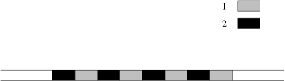
Figure 3:

From (58) we see that, when the operators $A_{k}$ all commute, the sequential and simultaneous weak values coincide. One important instance of this arises when the operators $A_{k}$ are applied to distinct subsystems, as in the case of the simultaneous weak measurements of the electron and positron in Hardy’s paradox Hardy (1992); Aharonov et al. (1991).

When the operators do not commute, the meaning of simultaneous weak measurement is not so obvious. One possible physical interpretation follows from the well-known formula

$$e^{X+Y}=\lim_{N\to\infty}(e^{X/N}e^{Y/N})^{N}$$ (60)

and its analogues for more operators. Suppose two pointers, one for $A_{1}$ and one for $A_{2}$, are coupled alternately in a sequence of $N$ short intervals (Figure 3, top diagram) with coupling strength $g_{k}/N$ for each interval. This is an enlarged sense of sequential weak measurement Mitchison et al. (2007) in which the same pointer is used repeatedly, coherently preserving its state between couplings. The state after post-selection is

$$\Psi_{\mathcal{M}}=\langle\psi_{f}|\left(e^{-i\left(\frac{g_{2}}{N}\right)s_{2}A_{2}}e^{-i\left(\frac{g_{1}}{N}\right)s_{1}A_{1}}\right)^{N}|\psi_{i}\rangle\phi_{1}(r_{1})\phi_{2}(r_{2}).$$ (61)

From (60) we deduce that

$$\Psi_{\mathcal{M}}\approx\langle\psi_{f}|e^{-i(g_{2}s_{2}A_{2}+g_{1}s_{1}A_{1})}|\psi_{i}\rangle\phi_{1}(r_{1})\phi_{2}(r_{2}).$$ (62)

This picture readily extends to more operators $A_{k}$.

One can also simulate a simultaneous measurement by averaging the results of a set of sequential measurements with the operators in all orders; in effect, one carries out a set of experiments that implement the averaging in (58). There is then no single act that counts as simultaneous measurement, but weak measurement in any case relies on averaging many repeats of experiments in order to extract the signal from the noise. In a certain sense, therefore, sequential measurement includes and extends the concept of simultaneous measurement. However, if we wish to accomplish simultaneous measurement in a single act, then we need a broader concept of weak measurement where pointers can be re-used; indeed, we can go further, and consider generalised weak coupling between one time-evolving system and another, followed by measurement of the second system. However, even in this case, the measurement results can be expressed algebraically in terms of the sequential weak values of the first system Mitchison et al. (2007).

VII Lowering operators

Lundeen and Resch Lundeen and Resch (2005) showed that, for a gaussian initial pointer wavefunction, if one defines an operator $a$ by

$$a_{LR}=\langle p^{2}\rangle_{i}^{1/2}\left(q+\frac{ip}{2\langle p^{2}\rangle_{i}}\right),$$

then the relationship

$$\langle a_{LR}\rangle=g\langle p^{2}\rangle_{i}^{1/2}A_{w}$$

holds. They argued that $a_{LR}$ can be interpreted physically as a lowering operator, carrying the pointer from its first excited state $|1\rangle$, in number state notation, to the gaussian state $|0\rangle$ (despite the fact that the pointer is not actually in a harmonic potential). Although $a_{LR}$ is not an observable, $\langle a_{LR}\rangle$ can be regarded as a prescription for combining expecations of pointer position and momentum to get the weak value.

If instead of $a_{LR}$ one takes

$$a=q+\frac{ip}{2\langle p^{2}\rangle_{i}},$$ (63)

then the even simpler relationship

$$\langle a\rangle=gA_{w},$$ (64)

holds. We refer to $a$ as a generalised lowering operator.

Lundeen and Resch also extended their lowering operator concept to simultaneous weak measurement of several observables $A_{k}$. Rephrased in terms of our generalised lowering operators $a_{k}$ defined by (63), their finding Lundeen and Resch (2005) can be stated as

$$\langle a_{1}\ldots a_{n}\rangle=g_{1}\ldots g_{n}(A_{1}\ldots A_{n})_{ws}.$$ (65)

This is of interest for two reasons. First, the entire simultaneous weak value appears on the right-hand side, not just its real part; and second, the “extra terms” in the simultaneous analogues of (54), (55) and (56) have disappeared. The lowering operator seems to relate directly to weak values.

We can generalise these ideas in two ways. First, we extend them from simultaneous to sequential weak measurements. Secondly, instead of assuming the initial pointer wavefunction is a gaussian, we allow it be arbitrary; we do this by defining a generalised lowering operator

$$a=q+i\frac{p}{\eta},\qquad\mbox{with}\qquad\eta=-i{\overline{\xi}}_{p}/{\overline{\xi}}_{q}.$$ (66)

For a gaussian $\phi$, $\eta=2\langle p^{2}\rangle_{i}$, so the above definition reduces to (63) in this case. In general, however, $\phi$ will not be annihilated by $a$ and is therefore not the number state $|0\rangle$ (this state is a gaussian with complex variance $\eta^{-1}$). Nonetheless, there is an analogue of Theorem IV.1 in which the whole sequential weak value, rather than its real part, appears:

Theorem VII.1 (Cumulant theorem for lowering operators).

For $n>1$

$$\langle a_{1}\ldots a_{n}\rangle^{c}=g_{1}\ldots g_{n}\ \vartheta\ (A_{n},\ldots A_{1})_{w}^{c},$$ (67)

where $\vartheta$ is given by

$$\vartheta=\sum_{(i_{1},\ldots i_{n})\in\{0,1\}^{n}}\ \frac{(-1)^{\sum i_{j}}\xi_{r_{i_{1}}\ldots r_{i_{n}}}\left({\overline{\xi}}_{r_{1-i_{1}}}\ldots{\overline{\xi}}_{r_{1-i_{n}}}\right)}{2\left({\overline{\xi}}_{p_{1}}\ldots{\overline{\xi}}_{p_{n}}\right)}.$$ (68)

For $n=1$ the same result holds, but with the extra term $\langle a\rangle_{i}$:

$$\langle a\rangle=\langle a\rangle_{i}+\vartheta gA_{w}.$$ (69)

Proof.

Put $r_{0}=q$, $r_{1}=p$. Then

$$\langle a_{1}\ldots a_{n}\rangle^{c} =\langle(q_{1}+ip_{1}/\eta_{1})\ldots(q_{n}+ip_{n}/\eta_{n})\rangle^{c},$$

$$=\sum_{(i_{1},\ldots i_{n})\in\{0,1\}^{n}}\ \frac{(-1)^{\sum i_{j}}\langle r_{i_{1}}\ldots r_{i_{n}}\rangle^{c}\left({\overline{\xi}}_{r_{1-i_{1}}}\ldots{\overline{\xi}}_{r_{1-i_{n}}}\right)}{\left({\overline{\xi}}_{p_{1}}\ldots{\overline{\xi}}_{p_{n}}\right)},$$

$$=g_{1}\ldots g_{n}\left[\vartheta(A_{n},\ldots A_{1})^{c}_{w}+\varpi(\overline{A_{n},\ldots A_{1}})^{c}_{w}\right],$$

where we used Theorem IV.1 to get the last line, and where $\vartheta$ is given by (68) and $\varpi$ by

$$\varpi=\sum_{(i_{1},\ldots i_{n})\in\{0,1\}^{n}}\ \frac{(-1)^{\sum i_{j}}{\overline{\xi}}_{r_{i_{1}}\ldots r_{i_{n}}}\left({\overline{\xi}}_{r_{1-i_{1}}}\ldots{\overline{\xi}}_{r_{1-i_{n}}}\right)}{2\left({\overline{\xi}}_{p_{1}}\ldots{\overline{\xi}}_{p_{n}}\right)};$$

(note the bar over ${\overline{\xi}}_{r_{i_{1}}\ldots r_{i_{n}}}$ that is absent in the definition of $\vartheta$ by (68)).

We want to prove $\varpi=0$, and to do this it suffices to prove that the complex conjugate of the numerator is zero, i.e.

$$\varpi^{\prime}=\sum_{(i_{1},\ldots i_{n})\in\{0,1\}^{n}}\ (-1)^{\sum i_{j}}\xi_{r_{i_{1}}\ldots r_{i_{n}}}\left(\xi_{r_{1-i_{1}}}\ldots\xi_{r_{1-i_{n}}}\right)=0.$$

Let $a_{k}=\langle q_{k}s_{k}\rangle_{i}$, $b_{k}=\langle q_{k}\rangle_{i}\langle s_{k}\rangle_{i}$, $c_{k}=\langle p_{k}s_{k}\rangle_{i}$, $d_{k}=\langle p_{k}\rangle_{i}\langle s_{k}\rangle_{i}$. Using the definition of $\xi$ in (25), the above equation can be written

$$\varpi^{\prime}/(2^{n+1}(-1)^{n}) =\prod_{k=1}^{n}\left\{a_{k}(c_{k}-d_{k})-c_{k}(a_{k}-b_{k})\right\}-\prod_{k=1}^{n}\left\{b_{k}(c_{k}-d_{k})-d_{k}(a_{k}-b_{k})\right\}$$

$$=\prod(b_{k}c_{k}-a_{k}d_{k})-\prod(b_{k}c_{k}-a_{k}d_{k})=0.$$

∎

Suppose the interaction Hamiltonian has the standard von Neumann form $H_{int}=gpA$, so $s=p$ in the definition of $\xi$ by equation (25). Then for $n=1$, since $\overline{\xi}_{p}=\xi_{p}$ and $\overline{\langle qp\rangle}_{i}=\langle pq\rangle_{i}$, $\vartheta=(-i)(\xi_{q}-\overline{\xi}_{q})=(-i)(\langle qp\rangle_{i}-\langle pq\rangle_{i})=1$, so we get the even simpler result

$$\langle a\rangle=\langle a\rangle_{i}+gA_{w}.$$ (70)

This is valid for all initial pointer wavefunctions, and therefore extends Lundeen and Resch’s equation (64). It seems almost too simple: there is no factor corresponding to $\xi$ in equation (46). However, a dependency on the initial pointer wavefunction is of course built into the definition of $a$ through $\eta$.

For $n>1$ it is no longer true that $\vartheta=1$, even with the standard interaction Hamiltonian. However, if in addition $\langle p\rangle_{i}=0$, then

$$\vartheta=(-i)^{n}\prod_{k=1}^{n}\left(\langle q_{k}p_{k}\rangle_{i}-\langle p_{k}q_{k}\rangle_{i}\right)=(-i)^{n}(i)^{n}=1.$$

Thus $\langle a_{1}\ldots a_{n}\rangle^{c}=g_{1}\ldots g_{n}(A_{n},\ldots A_{1})_{w}^{c}$ for all $n$. Applying the inverse operation for the cumulant, given by Propostion II.1, we deduce:

Corollary VII.2.

If $\langle p\rangle_{i}=0$, e.g. if the initial pointer wavefunction $\phi$ is real, then for $n>1$

$$\langle a_{1}\ldots a_{n}\rangle=g_{1}\ldots g_{n}(A_{n},\ldots A_{1})_{w}.$$ (71)

This is the sequential weak value version of the result for simultaneous measurements, (65), but is more general than the gaussian case treated in Lundeen and Resch (2005).

We might be tempted to try to repeat the above argument for pointer positions $q_{k}$ instead of the lowering operators $a_{k}$ by applying the anti-cumulant to both sides of (24). This fails, however, because of the need to take the real part of the weak values; in fact, this is one way of seeing where the extra terms come from in (54), (55) and (56) and their higher analogues.

Note also that (71) does not hold for general $\phi$, since then different subsets of indices may have different values of $\vartheta$.

VIII Discussion

The procedure for sequential weak measurement involves coupling pointers at several stages during the evolution of the system, measuring the position (or some other observable) of each pointer, and then multiplying the measured values together. In Mitchison et al. (2007) it was argued that we would really like to measure the product of the values of the operators $A_{1},\ldots A_{n}$, and that this corresponds to the sequential weak value $(A_{n},\ldots,A_{1})_{w}$. Multiplication of the values of pointer observables is the best we can do to achieve this goal. However, this brings along extra terms, such as $(A_{1})_{w}({\bar{A}}_{2})_{w}$ in (54), which are an artefact of this method of extracting information. From this perspective, the cumulant extracts the information we really want.

In Mitchison et al. (2007), a somewhat idealised measuring device was being considered, where the pointer position distribution is real and has zero mean. When the pointer distribution is allowed to be arbitrary, the expressions for $\langle q_{1}\ldots q_{n}\rangle$ become wildly complicated (see for instance (72)). Yet the cumulant of these terms condenses into the succinct equation (24) with all the complexity hidden away in the one number $\xi$. Why does the cumulant have this property?

Recall that the cumulant vanishes when its variables belong to two independent sets. The product of the pointer positions $q_{1},\ldots q_{n}$ will include terms that come from products of disjoint subsets of these pointer positions, and the cumulant of these terms will be sent to zero, by Lemma II.3. For instance, with $n=2$, the pointers are deflected in proportion to their individual weak values, according to (4), and the cumulant subtracts this component leaving only the component that arises from the $O(g^{2})$-influence of the weak measurement of $A_{1}$ on that of $A_{2}$. The subtraction of this component corresponds to the subtraction of the term $(A_{1})_{w}({\bar{A}}_{2})_{w}$ from (54). In general, the cumulant of pointer positions singles out the maximal correlation involving all the $q_{i}$, and the theorem tells us that this is directly related to the corresponding “maximal correlation” of sequential weak values, $(A_{n},\ldots,A_{1})^{c}$, which involves all the operators.

In fact, the theorem tells us something stronger: that it does not matter what pointer observable $r(p,q)$ we measure, e.g. position, momentum, or some Hermitian combination of them, and that likewise the coupling of the pointer with the system can be via a Hamiltonian $H_{int}=gs(p,q)A$ with any Hermitian $s(p,q)$. Different choices of $r$ and $s$ lead only to a different multiplicative constant $\xi$ in front of $(A_{n},\ldots,A_{1})_{w}^{c}$ in (24). We always extract the same function of sequential weak values, $(A_{n},\ldots,A_{1})_{w}^{c}$, from the system. This argues both for the fundamental character of sequential weak values and also for the key role played by their cumulants.

IX Acknowledgements

I am indebted to J. Åberg for many discussions and for comments on drafts of this paper; I thank him particularly for putting me on the track of cumulants. I also thank A. Botero, P. Davies, R. Jozsa, R. Koenig and S. Popescu for helpful comments. A preliminary version of this work was presented at a workshop on “Weak Values and Weak Measurement” at Arizona State University in June 2007, under the aegis of the Center for Fundamental Concepts in Science, directed by P. Davies.

Appendix A An explicit calculation

To calculate $\langle q_{1}q_{2}\rangle$ for arbitrary pointer wavefunctions $\phi_{1}$ and $\phi_{2}$, we use (28) to determine the state of the two pointers after the weak interaction, and then evaluate the expectation using (29), keeping only terms up to order $g^{2}$. We define

$$\mu_{k} =\langle q_{k}\rangle_{i},\ \ \nu_{k}=\langle p_{k}\rangle_{i},\ \ \zeta_{k}=\langle p_{k}^{2}\rangle_{i},$$

$$\rho_{k} =\langle q_{k}p_{k}\rangle_{i},\ \ \sigma_{k}=\langle q_{k}p_{k}^{2}\rangle_{i},\ \ \tau_{k}=\langle p_{k}q_{k}p_{k}\rangle_{i},$$

Then, expanding the exponential in (28) and substituting $\Psi$ in (29) gives, up to order $g^{2}$,

$$\langle q_{1}q_{2}\rangle =\mu_{1}\mu_{2}-ig_{1}\left\{\left((A_{1})_{w}-({\bar{A}}_{1})_{w}\right)\mu_{1}\nu_{1}\mu_{2}-({\bar{A}}_{1})_{w}{\bar{\rho}}_{1}\mu_{2}+(A_{1})_{w}\rho_{1}\mu_{2}\right\}$$ (72)

$$-ig_{2}\left\{\left((A_{2})_{w}-({\bar{A}}_{2})_{w}\right)\mu_{1}\mu_{2}\nu_{2}-({\bar{A}}_{2})_{w}\mu_{1}{\bar{\rho}}_{2}+(A_{2})_{w}\mu_{1}\rho_{2}\right\}$$

$$+g_{1}^{2}\left\{|(A_{1})_{w}|^{2}(\tau_{1}\mu_{2}-\mu_{1}\zeta_{1}\mu_{2})+\left((A_{1}^{2})_{w}+({\bar{A}}_{1}^{2})_{w}\right)\frac{\mu_{1}\zeta_{1}\mu_{2}}{2}\right\}$$

$$-g_{1}^{2}\left\{\left((A_{1})_{w}-({\bar{A}}_{1})_{w}\right)^{2}\mu_{1}\nu_{1}^{2}\mu_{2}+(A_{1}^{2})_{w}\frac{\sigma_{1}\mu_{2}}{2}+({\bar{A}}_{1}^{2})_{w}\frac{{\bar{\sigma}_{1}}\mu_{2}}{2}\right\}$$

$$+g_{2}^{2}\left\{|(A_{2})_{w}|^{2}(\mu_{1}\tau_{2}-\mu_{1}\mu_{2}\zeta_{2})+\left((A_{2}^{2})_{w}+({\bar{A}}_{2}^{2})_{w}\right)\frac{\mu_{1}\mu_{2}\zeta_{2}}{2}\right\}$$

$$-g_{2}^{2}\left\{\left((A_{2})_{w}-({\bar{A}}_{w})_{2}\right)^{2}\mu_{1}\mu_{2}\nu_{2}^{2}+(A_{2}^{2})_{w}\frac{\mu_{1}\sigma_{2}}{2}+({\bar{A}}_{2}^{2})_{w}\frac{\mu_{1}{\bar{\sigma}_{2}}}{2}\right\}$$

$$+g_{1}g_{2}\left\{(A_{1})_{w}({\bar{A}}_{2})_{w}\rho_{1}{\bar{\rho}_{2}}+({\bar{A}}_{1})_{w}(A_{2})_{w}{\bar{\rho}_{1}}\rho_{2}-(A_{2},A_{1})_{w}\rho_{1}\rho_{2}-\overline{(A_{2},A_{1})}_{w}{\bar{\rho}}_{1}{\bar{\rho}}_{2}\right\}$$

$$-g_{1}g_{2}\left\{2\left((A_{1})_{w}-({\bar{A}}_{1})_{w}\right)\left((A_{2})_{w}-({\bar{A}}_{2})_{w}\right)\mu_{1}\nu_{1}\mu_{2}\nu_{2}\right\}$$

$$+g_{1}g_{2}\left\{\left((A_{2},A_{1})_{w}+\overline{(A_{2},A_{1})}_{w}-(A_{1})_{w}({\bar{A}}_{2})_{w}-({\bar{A}}_{1})_{w}(A_{2})_{w}\right)\mu_{1}\nu_{1}\mu_{2}\nu_{2}\right\}$$

$$+g_{1}^{2}\left\{\left((A_{1})_{w}-({\bar{A}}_{1})_{w}\right)(A_{1})_{w}\nu_{1}\rho_{1}\mu_{2}-\left((A_{1})_{w}-({\bar{A}}_{1})_{w}\right)({\bar{A}_{1}})_{w}\nu_{1}{\bar{\rho}}_{1}\mu_{2}\right\}$$

$$+g_{2}^{2}\left\{\left((A_{2})_{w}-({\bar{A}}_{2})_{w}\right)(A_{2})_{w}\mu_{1}\nu_{2}\rho_{2}-\left((A_{2})_{w}-({\bar{A}}_{2})_{w}\right)({\bar{A}}_{2})_{w}\mu_{1}\nu_{2}{\bar{\rho}_{2}}\right\}$$

$$+g_{1}g_{2}\left\{\left((A_{1})_{w}-({\bar{A}}_{1})_{w}\right)(A_{2})_{w}\mu_{1}\nu_{1}\rho_{2}-\left((A_{1})_{w}-({\bar{A}}_{1})_{w}\right)({\bar{A}}_{2})_{w}\mu_{1}\nu_{1}{\bar{\rho}_{2}}\right\}$$

$$+g_{1}g_{2}\left\{\left((A_{2})_{w}-({\bar{A}}_{2})_{w}\right)(A_{1})_{w}\rho_{1}\mu_{2}\nu_{2}-\left((A_{2})_{w}-({\bar{A}}_{2})_{w}\right)({\bar{A}}_{1})_{w}{\bar{\rho}_{1}}\mu_{2}\nu_{2}\right\}.$$

To calculate the cumulant $\langle q_{1},q_{2}\rangle^{c}=\langle q_{1}q_{2}\rangle-\langle q_{1}\rangle\langle q_{2}\rangle$ we need $\langle q\rangle$ up to order $g^{2}$:

$$\langle q\rangle =\mu+ig\left\{A_{w}(\mu\nu-\rho)-{\bar{A}}_{w}(\mu\nu-{\bar{\rho}})\right\}+g^{2}|A_{w}|^{2}\left(\tau-\mu\zeta+2\mu\nu^{2}-\nu\rho-\nu{\bar{\rho}}\right)$$ (73)

$$+g^{2}\left\{(A^{2})_{w}\left(\frac{\mu\zeta}{2}-\frac{\sigma}{2}\right)-({\bar{A}}^{2})_{w}\left(\frac{\mu\zeta}{2}-\frac{\bar{\sigma}}{2}\right)+(A_{w})^{2}(\nu\rho-\mu\nu^{2})+({\bar{A}}_{w})^{2}(\nu{\bar{\rho}}-\mu\nu^{2})\right\}.$$

Substituting from (72) and (73) a radical simplification occurs:

$$\langle q_{1}q_{2}\rangle^{c}=g_{1}g_{2}\left\{(A_{2},A_{1})_{w}-(A_{1})_{w}(A_{2})_{w}\right\}\left(\mu_{1}\nu_{1}\mu_{2}\nu_{2}-\rho_{1}\rho_{2}\right)+\mbox{complex conjugate}.$$ (74)

This, of course, is what Theorem IV.1 tells us.

References

• Jozsa (2007) R. Jozsa (2007), eprint quant-ph/0706.4207.
• Mitchison et al. (2007) G. Mitchison, R. Jozsa, and S. Popescu (2007), eprint quant-ph/0706.150.
• Aharonov and Rohrlich (2005) Y. Aharonov and D. Rohrlich, Quantum Paradoxes (Wiley-VCH, Weinheim, Germany, 2005).
• Aharonov et al. (1988) Y. Aharonov, D. Z.Albert, and L. Vaidman, Phys. Rev. Lett. 60, 1351 (1988).
• Oreshkov and A.Brun (2005) O. Oreshkov and T. A.Brun, Question 0, 0 (2005).
• Bennett et al. (1999) C. H. Bennett, D. P. DiVincenzo, C. Fuchs, T. Mor, E. Rains, P. W. Shor, J. A. Smolin, and W. K. Wootters, Phys. Rev. A 59, 1070 (1999).
• von Neumann (1955) J. von Neumann, Mathematische Grundlagen der Quantenmechanik (Springer Berlin 1932; English translation Princeton University Press, Princeton, 1955).
• Kendall and Stuart (1977) M. Kendall and A. Stuart, The advanced theory of statistics, Volume 1 (Charles Griffin, London and High Wycombe, 1977).
• Royer (1983) A. Royer, J. Math. Phys. 24, 897 (1983).
• Zhou et al. (2006) D. L. Zhou, B. Zeng, Z. Xu, and L. You, Phys. Rev. A 74, 052110 (2006).
• Apostol (1976) T. M. Apostol, Introduction to analytic number theory (Springer-Verlag, New York, 1976).
• Percus (1975) J. K. Percus, Commun. math. Phys. 40, 283 (1975).
• Simon (1979) B. Simon, Functional integration and quantum physics (Academic Press, New York, San Francisco, London, 1979).
• Resch and Steinberg (2004) K. J. Resch and A. M. Steinberg, Phys. Rev. Lett. 92, 130402 (2004).
• Resch (2004) K. J. Resch, J. Opt. B: Quantum Semiclass. Opt. 6, 482 (2004).
• Lundeen and Resch (2005) J. S. Lundeen and K. J. Resch, Phys. Lett. A 334, 337 (2005).
• Hardy (1992) L. Hardy, Phys. Rev. Lett. 68, 2981 (1992).
• Aharonov et al. (1991) Y. Aharonov, A. Botero, S. Popescu, B. Reznik, and J. Tollaksen, in Proceedings of NATO ARW Mykonos 2000 Decoherence and its implications in quantum computation and information transfer: [proceedings of the NATO advanced research workshop, Mykonos, Greece, 25-30.06.2000], edited by A. Gonis and P. Turchi (IOS Press, 1991).