A New Algorithm in Geometry of Numbers

Abstract

A lattice Delaunay polytope $P$ is called perfect if its Delaunay sphere is the only ellipsoid circumscribed about $P$. We present a new algorithm for finding perfect Delaunay polytopes. Our method overcomes the major shortcomings of the previously used method [Du05]. We have implemented and used our algorithm for finding perfect Delaunay polytopes in dimensions 6, 7, 8. Our findings lead to a new conjecture that sheds light on the structure of lattice Delaunay tilings.

1 Introduction

Let $\Lambda$ be an $n$-dimensional lattice ($n\geq 0$) and let $P\subset\Lambda\otimes\mathbb{R}\cong\mathbb{R}^{n}$ be a polytope whose vertex set $\operatorname{\mathsf{vert}}P$ belongs to $\Lambda$. We say that $P$ is a Delaunay polytope for $\Lambda$ if $P$ can be circumscribed by a closed ball $\mathcal{B}_{P}\subset\Lambda\otimes\mathbb{R}$ such that $\mathcal{B}_{P}\cap\Lambda=\operatorname{\mathsf{vert}}P$. The ball $\mathcal{B}_{P}$ (or its boundary) is commonly referred to as the Delaunay sphere (or empty sphere) for $P$. (Delaunay [Del] himself attributed the concept of empty sphere to Voronoi.) Delaunay polytopes for $\Lambda$ form a face-to-face tiling of $\Lambda\otimes\mathbb{R}$ called the Delaunay tiling for $\Lambda$.

One can study the geometry of lattices by comparing their Delaunay tilings. Such study was initiated by Voronoi [VorII08-09]. As $\Lambda\subset\Lambda\otimes\mathbb{R}\cong\mathbb{R}^{n}$ is deformed into $\mathbb{Z}^{n}\subset\mathbb{R}^{n}$ by an affine transformation $\mbox{\boldmath$x$}\mapsto A(\mbox{\boldmath$x$})$, the empty spheres circumscribed about the Delaunay polytopes of $\Lambda$ are deformed into empty ellipsoids circumscribed about the $A$-images of these polytopes. All these ellipsoids have identical quadratic parts – indeed they are balls in the metric $d(\mbox{\boldmath$x$},\mbox{\boldmath$x$}^{\prime})=||A^{-1}(\mbox{\boldmath$x$})-A^{-1}(\mbox{\boldmath$x$}^{\prime})||$. Thus, the study of Delaunay tilings for $n$-lattices is equivalent to the study of Delaunay tilings for $\mathbb{Z}^{n}$ with respect to different positive definite quadratic forms. Let us denote the Delaunay tiling for $\mathbb{Z}^{n}$ with respect to a positive quadratic form $\mathcal{Q}$ by $Del(\mathbb{Z}^{n},\mathcal{Q})$. The Delaunay property of an ellipsoid $\mathcal{E}(\mathcal{Q},\mbox{\boldmath$c$},R)=\{\mbox{\boldmath$x$}\in\mathbb{R}^{n}\;|\;\mathcal{Q}[\mbox{\boldmath$x$}-\mbox{\boldmath$c$}]\leq R^{2}\}$, circumscribed about a polytope $P$, means that the quadratic function $\mathcal{Q}[\mbox{\boldmath$x$}-\mbox{\boldmath$c$}]-R^{2}$ is zero on $\operatorname{\mathsf{vert}}P$ and strictly positive on $\mathbb{Z}^{n}\setminus\operatorname{\mathsf{vert}}P$. From now on we will be working with $\Lambda=\mathbb{Z}^{n}$, unless stated otherwise.

It is natural to extend the notions of Delaunay polytope and tiling to positive semidefinite forms. We refer to an $\mathbb{R}$-valued function $f$ on a set $S$ as positive if $f(x)\geq 0$ for any $x\in S$. Let $\mathcal{Q}$ be a quadratic form that is positive on $\mathbb{R}^{n}$ and such that the rank of the sublattice $\ker_{\mathbb{R}}\mathcal{Q}\cap\mathbb{Z}^{n}$ is equal to the dimension of $\ker_{\mathbb{R}}\mathcal{Q}$. Then $\mathbb{R}^{n}$ is tiled by unbounded $n$-dimensional polyhedra, which are Delaunay with respect to $\mathcal{Q}$: each polyhedron $P$ from this family is circumscribed by an elliptic cylinder $\mathcal{E}_{P}$, whose interior is free of lattice points, so that $P\cap\mathbb{Z}^{n}=\mathcal{E}_{P}\cap\mathbb{Z}^{n}$. Furthermore, $P$ is the direct affine product of a Delaunay polytope $P$ for a sublattice $\Lambda\subset\mathbb{Z}^{n}$ of rank $r=\dim\ker_{\mathbb{R}}\mathcal{Q}$ and an affine $(n-r)$-subspace of $\mathbb{R}^{n}$. The degenerate Delaunay “ellipsoid” $\mathcal{E}_{P}$ for an unbounded polyhedron $P$ is the direct affine product of the Delaunay ellipsoid for $P$ and $L$; we will be using ‘ellipsoid’ for both bounded and unbounded ellipsoids. For example, $\mathbb{R}^{n}$ is tiled by the unit slabs $U_{i}=\{\mbox{\boldmath$x$}\;\vline\;i\leq x_{1}\leq i+1\}$ where $i\in\mathbb{Z}$. Each unit slab is a Delaunay polyhedron with respect to quadratic form $x_{1}^{2}$; furthermore, each $U_{i}$ coincides with its Delaunay ellipsoid $\mathcal{E}_{U_{i}}$. Following a common convention we will be using the word ‘polytope’ only for bounded polyhedra.

Let $\Lambda$ be a lattice of rank $n$ and let $P\subset\Lambda\otimes\mathbb{R}$ be a lattice polyhedron, i.e., the convex hull of a subset of $\Lambda$. Then $P$ is called perfect if there is an $n$-ellipsoid (possibly degenerate) circumscribed about $P$ and this ellipsoid is unique. Perfect Delaunay polyhedra are also called extreme (e.g. [Du05]). Perfect Delaunay polytopes are rare in small dimensions, e.g., for $n\leq 6$ there are only three such polytopes – $0$ for $n=0$, $[0,1]$ for $n=1$, and Gosset’s semiregular polytope $2_{21}$ for $n=6$. The previous method [Du05] for finding perfect Delaunay polytopes was based on an unproven conjecture that every perfect Delaunay polytope is basic. A lattice polytope $P$ is called basic if there exist $v_{0},\dots,v_{n}\in\operatorname{\mathsf{vert}}P$ such that every $v\in\operatorname{\mathsf{vert}}P$ can be written as $v=\sum_{i=0}^{n}\lambda_{i}v_{i}$ where $\lambda_{1},\dots,\lambda_{n+1}\in\mathbb{Z}$ and $1=\sum_{i=0}^{n}\lambda_{i}$. We know that there exist non-basic Delaunay polytopes in higher dimensions (see [DG07]) and we cannot rule out the existence of non-basic perfect Delaunay polytopes.

The perfection property of a Delaunay polytope $P$ with ellipsoid $\mathcal{E}(\mathcal{Q},\mbox{\boldmath$c$},\rho)=\{\mbox{\boldmath$x$}\in\mathbb{R}^{n}\;|\;\mathcal{Q}[\mbox{\boldmath$x$}-\mbox{\boldmath$c$}]\leq\rho^{2}\}$ amounts to that any quadratic function that vanishes on $\operatorname{\mathsf{vert}}P$ is of the form $\alpha(\mathcal{Q}[\mbox{\boldmath$x$}-\mbox{\boldmath$c$}]-\rho^{2})$ where $\alpha\in\mathbb{R}$. A real-valued quadratic function $F$ on $\mathbb{R}^{n}$ is called perfect if $\operatorname{armin}F=\min\{F(\mbox{\boldmath$z$})\;\vline\;\mbox{\boldmath$z$}\in\mathbb{Z}^{n}\}\geq 0$ and $\operatorname{\mathsf{conv}}\{\mbox{\boldmath$z$}\in\mathbb{Z}^{n}\;\vline\;F(\mbox{\boldmath$z$})=\operatorname{armin}F\}$ is a perfect Delaunay polyhedron. The ellipsoid $\{\mbox{\boldmath$x$}\in\mathbb{R}^{n}\;\vline\;F(\mbox{\boldmath$x$})\leq\operatorname{armin}F\}$ is also called perfect.

Erdahl proved that the vertex set of any perfect Delaunay polyhedron splits uniquely (up to arithmetic equivalence) into the direct affine sum of the vertex set of a perfect Delaunay polytope and a sublattice which is parallel to the kernel of $\mathcal{Q}$ [Er92].

Theorem 1

[Er92] A polyhedron $P\in Del(\mathbb{Z}^{n},\mathcal{Q})$ is perfect if and only if

$$P\cap\mathbb{Z}^{n}=\{v+\mbox{\boldmath$z$}\;\vline\;v\in\operatorname{\mathsf{vert}}D,\>\mbox{\boldmath$z$}\in\Gamma\},$$

where $D$ is a perfect polytope from $Del(\mathbb{Z}^{n}\cap\operatorname{\mathsf{aff}}D,\mathcal{Q})$ and $\Gamma$ is a submodule of $\mathbb{Z}^{n}$ such that $\mathbb{Z}^{n}$ is the direct sum of modules $(\mathbb{Z}^{n}\cap\operatorname{\mathsf{aff}}D)-(\mathbb{Z}^{n}\cap\operatorname{\mathsf{aff}}D)$ and $\Gamma$. If $(D^{\prime},\Gamma^{\prime})$ is another pair with these properties, then $\Gamma^{\prime}=\Gamma$ and $D^{\prime}=A(D)$, where $A$ is an affine automorphism of $\mathbb{Z}^{n}$.

The fundamental importance of perfect Delaunay polyhedra is explained by the following theorem of Erdahl [E00].

Theorem 2

Let $D$ be a Delaunay polytope for $\mathbb{Z}^{n}$. Then

$$D=\bigcap_{i=1}^{k}P_{i},$$

where each $P_{i}$ is a perfect Delaunay polyhedron for $\mathbb{Z}^{n}$ with respect to some positive form $\mathcal{Q}_{i}$ such that $\dim\ker_{\mathbb{R}}\mathcal{Q}_{i}=\operatorname{rank}(\ker_{\mathbb{R}}\mathcal{Q}_{i}\cap\mathbb{Z}^{n})$.

For $S\subset\mathbb{Z}^{n}$ we define $\operatorname{\mathsf{qrank}}S$, the quadratic rank of $S$, as the dimension of the space of quadratic functions on $\mathbb{R}^{n}$ that vanish on $S$. Let $P$ and $P_{1}$ be two perfect Delaunay polytopes for $\mathbb{Z}^{n}$ such that $\operatorname{\mathsf{qrank}}(\operatorname{\mathsf{vert}}P\cap\operatorname{\mathsf{vert}}P_{1})=2$. In this case we call $P$ and $P_{1}$ adjacent. If two perfect Delaunay $n$-polytopes $P$ and $P^{\prime}$ can be connected by a sequence of perfect Delaunay $n$-polytopes in which every two consecutive members are adjacent, then we will say that $P$ and $P^{\prime}$ belong to the same adjacency component. We developed a method for finding an adjacency component for a perfect Delaunay polytope. We have found that for each $n\leq 8$ all known perfect Delaunay $n$-polytopes belong to the same adjacency component. This finding makes compelling the following conjecture.

Conjecture 1

For any $n\in\mathbb{N}$ all perfect Delaunay $n$-polytopes belong to the same adjacency component.

2 Space of quadratic functions

Let us denote by $\operatorname{\textsf{Sym}}(n)$ the space of real symmetric $n\times n$ matrices; by interpreting an element of $\operatorname{\textsf{Sym}}(n)$ as a Gram matrix, we can regard $\operatorname{\textsf{Sym}}(n)$ as the space of quadratic forms with real coefficients. Denote by $\textsf{Q}(n)$ the linear space of quadratic functions on $\mathbb{R}^{n}$ and by $\textsf{Q}_{0}(n)\subset\textsf{Q}(n)$ the subspace of functions with zero constant term. Since a quadratic function can be represented uniquely as the sum of a quadratic form, a linear functional, and a constant, it is convenient to introduce the projection operators

$$\operatorname{Quad}:\textsf{Q}(n)\rightarrow\operatorname{\textsf{Sym}}(n),\;\operatorname{Lin}:\textsf{Q}(n)\rightarrow{\mathbb{R}^{n}}^{*},\;$$

$$\operatorname{Const}:\textsf{Q}(n)\rightarrow\mathbb{R}.$$

For two quadratic forms with Gram matrices $\mathbf{A}$ and $\mathbf{B}$ we define the dot product on $\operatorname{\textsf{Sym}}(n)$ as $\operatorname{trace}(\mathbf{A}\mathbf{B})$. For linear functions defined by covectors $a$ and $b$ the dot product is just $a\cdot b$. The dot product on $\textsf{Q}_{0}(n)$ is defined as the direct sum of the dot products on $\operatorname{\textsf{Sym}}(n)$ and ${\mathbb{R}^{n}}^{*}$.

The main idea of this paper is in interpreting quadratic functions on $\mathbb{R}^{n}$ as elements of $\textsf{Q}_{0}(n)^{*}$, the dual of $\textsf{Q}_{0}(n)$. There is a natural correspondence between ellipsoids in $\mathbb{R}^{n}$ and closed (affine) halfspaces of $\textsf{Q}_{0}(n)$. Namely, if $\mathcal{E}=\{\mbox{\boldmath$x$}\in\mathbb{R}^{n}\;|\;\mathcal{Q}[\mbox{\boldmath$x$}-\mbox{\boldmath$c$}]\leq\rho^{2}\}$, then the corresponding halfspace $H_{\mathcal{E}}$ is $\{X\in\textsf{Q}_{0}(n)\;|\;X\cdot F\geq\rho^{2}-\mathcal{Q}[\mbox{\boldmath$c$}]\}$, where $F$ is the quadratic function defined by $F(\mbox{\boldmath$x$})=\mathcal{Q}[\mbox{\boldmath$x$}]-2\mathcal{Q}(\mbox{\boldmath$x$},\mbox{\boldmath$c$})$.

Let $\mathcal{D}$ be a map from $\mathbb{R}^{n}$ into $\textsf{Q}_{0}(n)$ defined in the matrix notation by

$$\mathcal{D}:\mbox{\boldmath$u$}\mapsto(\mbox{\boldmath$x$}\mapsto\mbox{\boldmath$x$}^{T}(\mbox{\boldmath$u$}\mbox{\boldmath$u$}^{T})\mbox{\boldmath$x$}+\mbox{\boldmath$u$}^{T}\mbox{\boldmath$x$}),$$

where $x$ and $u$ are treated as column vectors. Obviously, $\mathcal{D}$ takes an integer vector to a quadratic function with integer Gram matrix and integer linear part; such quadratic function is called classically integer. The map $\mathcal{D}$ resembles the Voronoi map $\mathcal{V}:\mathbb{R}^{n}\rightarrow\operatorname{\textsf{Sym}}(n)$ that takes a vector $u$ to the quadratic form with Gram matrix $\mbox{\boldmath$u$}\mbox{\boldmath$u$}^{T}$ (see [RB79] for details). Thus, we have $\mathcal{D}(\mbox{\boldmath$u$})=\mathcal{V}(\mbox{\boldmath$u$})+\mbox{\boldmath$u$}^{*}$, where $\mbox{\boldmath$u$}^{*}$ is linear functional dual to $u$. The map $\mathcal{V}$ can be seen as the quadratic Veronese map from $\mathbb{R}^{n}$ to $\operatorname{\textsf{Sym}}(n)$, although in contemporary literature the Veronese map is usually defined in the projective setup. We call an ellipsoid in $\mathbb{R}^{n}$ empty if its interior is free of points of $\mathbb{Z}^{n}$. If $\mathcal{E}=\{\mbox{\boldmath$x$}\in\mathbb{R}^{n}\;|\;\mathcal{Q}[\mbox{\boldmath$x$}-\mbox{\boldmath$c$}]\leq\rho^{2}\}$ is an empty ellipsoid, then $H_{\mathcal{E}}$ contains all of $\mathcal{D}(\mathbb{Z}^{n})$. Thus, $\mathcal{D}(\mathbb{Z}^{n})\subset\underset{\{\mathcal{E}\>\textrm{is\> empty}\}}{\bigcap}H_{\mathcal{E}}$. The right hand side is the intersection of infinitely many halfspaces, which can be replaced by the intersection of only those halfspaces whose boundaries are completely determined by the elements of $\mathcal{D}(\mathbb{Z}^{n})$ that lie on them. Throughout the paper we use $\operatorname{\mathsf{conv}}S$ to denote the convex hull of a set $S\subset\mathbb{R}^{n}$ and $\operatorname{\mathsf{aff}}S$ to denote the minimal affine subspace containing $S$.

We define the Erdahl polyhedron $\operatorname{E}(n)$ as the intersection of closed halfspaces $H_{\mathcal{E}}$ such that $\mathcal{E}$ is empty and $\operatorname{rank}(\partial H_{\mathcal{E}}\cap\mathcal{D}(\mathbb{Z}^{n}))=\dim\textsf{Q}_{0}(n).$

Theorem 3

The set $\mathcal{D}(\mathbb{Z}^{n})$ coincides with $\mathcal{D}(\mathbb{R}^{n})\cap\partial{\operatorname{E}}(n)$. Furthermore,

$$\operatorname{\mathsf{conv}}\mathcal{D}(\mathbb{Z}^{n})=\operatorname{E}(n).$$

Proof.   Each $\mbox{\boldmath$z$}\in\mathbb{Z}^{n}$ belongs to the boundary of an empty degenerate ellipsoid

$$\mathcal{E}=\{\mbox{\boldmath$x$}\in\mathbb{R}^{n}\;\;\vline\;\;\mbox{\boldmath$z$}\cdot\mbox{\boldmath$e$}_{1}\leq\mbox{\boldmath$x$}\cdot\mbox{\boldmath$z$}\leq\mbox{\boldmath$z$}\cdot\mbox{\boldmath$e$}_{1}+1\}.$$

It is easy to check that $\partial\mathcal{E}$ is the only quadratic surface passing through $\mathbb{Z}^{n}\cap\partial\mathcal{E}$ (or see [Er92] for a proof). Thus, $\operatorname{rank}\partial H_{\mathcal{E}}\cap\mathcal{D}(\mathbb{Z}^{n})=\dim\textsf{Q}_{0}(n)$ and $\mathcal{D}(\mathbb{Z}^{n})\subset\partial{\operatorname{E}}(n)$.

Let $X\in\mathcal{D}(\mathbb{R}^{n})\cap\partial{\operatorname{E}}(n)$. Then there is $\mbox{\boldmath$x$}\in\mathbb{R}^{n}$ with $X=\mathcal{D}(\mbox{\boldmath$x$})$. If $\mbox{\boldmath$x$}\notin\mathbb{Z}^{n}$ (for $\mbox{\boldmath$x$}\in\mathbb{Z}^{n}$ see above), then $\mbox{\boldmath$x$}=\mbox{\boldmath$u$}+\mbox{\boldmath$x$}^{\prime}$, where $\mbox{\boldmath$u$}\in\mathbb{Z}^{n}$ and $\mbox{\boldmath$x$}^{\prime}\in[0,1]^{n}$. Without loss of generality assume that $x_{1}^{\prime}\notin\mathbb{Z}$. Then $\mbox{\boldmath$x$}\in\operatorname{int}\mathcal{E}$, where $\mathcal{E}=\{\mbox{\boldmath$x$}\;\vline\;u_{1}\leq x_{1}\leq u_{1}+1\}$, which means $X\notin H_{\mathcal{E}}$, contradicting our choice of $X$. Thus, the only points of $\mathbb{R}^{n}$ that are mapped by $\mathcal{D}$ on $\partial\operatorname{E}(n)$ are elements of $\mathbb{Z}^{n}$ and the first claim of the theorem is proven.

Suppose $X\in\operatorname{E}(n)$ and let us show $X\in\operatorname{\mathsf{conv}}\mathcal{D}(\mathbb{Z}^{n})$. It is enough to prove this implication for $X\in\partial\operatorname{E}(n)$. If $X\in\partial\operatorname{E}(n)$, then $X$ lies on some $H_{\mathcal{E}}$, where $\mathcal{E}$ is empty and completely determined by elements of $\mathbb{Z}^{n}$ that lie on its boundary. If $X\notin\operatorname{\mathsf{conv}}\mathcal{D}(\mathcal{E}\cap\mathbb{Z}^{n})$, then there is a facet $C$ of $\operatorname{\mathsf{conv}}\mathcal{D}(\mathcal{E}\cap\mathbb{Z}^{n})$ such that $X$ and the relative interior of $\operatorname{\mathsf{conv}}\mathcal{D}(\mathcal{E}\cap\mathbb{Z}^{n})$ lie in the different halfspaces of $H_{\mathcal{E}}$ with respect to $\operatorname{\mathsf{aff}}C$. Let $f_{\mathcal{E}}(x)\geq 0$ be an affine inequality defining $H_{\mathcal{E}}$ and let $g_{C}(x)=0$ be an affine equation of the hyperplane passing through the point $I$ (where $I:\mbox{\boldmath$x$}\mapsto\mbox{\boldmath$x$}^{T}\mbox{\boldmath$x$}$) and $\operatorname{\mathsf{aff}}C$ such that $g_{C}(X)<0$. The equation of any hyperplane in $\textsf{Q}_{0}(n)$ passing through $\operatorname{\mathsf{aff}}C$ can be written as $f_{\mathcal{E}}(x)+\theta g_{C}(x)=0$ for some $\rho\in\mathbb{R}$. Let us define

$$\theta_{m}=\sup\{\theta\in\mathbb{R}\;\;\vline\;\;\forall\mbox{\boldmath$z$}\in\mathbb{Z}^{n}\,f_{\mathcal{E}}(\mathcal{D}(\mbox{\boldmath$z$}))+\theta g_{C}(\mathcal{D}(\mbox{\boldmath$z$}))\geq 0\}$$

We claim that $\theta_{m}>0$ and there exists $\mbox{\boldmath$u$}\in\mathbb{Z}^{n}\setminus E$ such that

$$f_{\mathcal{E}}(\mathcal{D}(\mbox{\boldmath$u$}))+\theta_{m}g_{C}(\mathcal{D}(\mbox{\boldmath$u$}))=0.$$

The proof of these claims (which we omit due to the space limitations) is based on standard techniques of geometry of numbers and follows the line of argument used by Voronoi in his first memoir [VorCol, Pages 177–179]. $\Box$

If an ellipsoid $\mathcal{E}$ is empty and $\partial H_{\mathcal{E}}$ contains $\dim\textsf{Q}_{0}(n)+1$ affinely independent points, then $\mathcal{E}$ is uniquely determined by the points of $\mathbb{Z}^{n}$ that lie on its boundary: in this case $\mathcal{E}$ is called a perfect ellipsoid for lattice $\mathbb{Z}^{n}$. Perfect ellipsoids were introduced by Erdahl [Er75, Er92]. Thus,

$$\operatorname{E}(n)=\operatorname{\mathsf{conv}}\mathcal{D}(\mathbb{Z}^{n})=\underset{\{E\>\textrm{is\> perfect}\}}{\bigcap}H_{\mathcal{E}}\>.$$

Note that $\operatorname{E}(n)$ is not a polyhedron in the sense of linear programming, where the number of constrains is always assumed to be finite. We will refer to the faces of $\operatorname{E}(n)$ of dimension $\dim\textsf{Q}_{0}(n)-1$ as facets and the facets of dimension $\dim\textsf{Q}_{0}(n)-1$ as faces. The facets of $\operatorname{E}(n)$ correspond to perfect Delaunay polyhedra. The bounded facets of $\operatorname{E}(n)$ correspond to perfect Delaunay polytopes. Two perfect Delaunay polytopes are adjacent if the corresponding facets of $\operatorname{E}(n)$ share a bounded ridge. Faces of $\operatorname{E}(n)$ correspond to Delaunay polyhedra – bounded faces to bounded Delaunay polyhedra (polytopes) and unbounded faces to unbounded polyhedra. There is a great deal of analogy between $\operatorname{E}(n)$ and Voronoi’s polyhedron $\Pi(n)$, introduced by Venkov [Ven40] (see also [RB79]). Recall that $\Pi(n)$ is defined as the convex hull of $\{\mathcal{V}(\mbox{\boldmath$p$})\;|\;\mbox{\boldmath$p$}\in\mathbb{Z}^{n}\;\textrm{and}\;g.c.d.(p_{1},\ldots,p_{n})=1\}$, where $\mathcal{V}:\mathbb{R}^{n}\rightarrow\operatorname{\textsf{Sym}}(n,\mathbb{R})$ is the Voronoi map. The facets of $\Pi(n)$ are defined by closed halfspaces corresponding to perfect forms, which were studied by Voronoi [VorI08] (part I). The bounded facets of $\Pi(n)$ correspond to positive definite perfect forms.

2.1 Geometry of $\operatorname{E}(n)$

Denote by $Aff_{n}(\mathbb{Z})$ the group of affine automorphisms of $\mathbb{Z}^{n}$, i.e. the group of transformations of the form $A(\mbox{\boldmath$z$})=L\mbox{\boldmath$z$}+\mbox{\boldmath$t$}$, where $L\in GL_{n}(\mathbb{Z})$ and $\mbox{\boldmath$t$}\in\mathbb{Z}^{n}$. The action of $Aff_{n}(\mathbb{Z})$ on $\mathbb{R}^{n}$ can be naturally lifted to $\textsf{Q}_{0}(n)$ by

$$F\mapsto\{\mbox{\boldmath$x$}\mapsto F(A^{-1}(\mbox{\boldmath$x$}))\}.$$

The group $Aff_{n}(\mathbb{Z})$ acts on $\operatorname{E}(n)$ in a way somewhat similar to that of $GL_{n}(\mathbb{Z})$ acting on $\Pi(n)$. Subsets $V$ and $V^{\prime}$ of $\mathbb{R}^{n}$ are called arithmetically equivalent if there exists $A\in Aff_{n}(\mathbb{Z})$ such that $A(V)=V^{\prime}$. Obviously, arithmetic equivalence preserves properties of ellipsoids such as the Delaunay property, emptiness, and perfection. Since there are only finitely many arithmetically distinct Delaunay polytopes in each dimension (e.g. [DL97]), the boundary of $\operatorname{E}(n)$ has finitely many distinct arithmetic types of faces. In fact, the definition of perfect ellipsoid implies that arithmetically equivalent perfect ellipsoids are isometric.

There are beautiful connections between the polytope $\operatorname{E}(n)$ and Delaunay tilings of $\mathbb{Z}^{n}$. The projection $\operatorname{Lin}:\textsf{Q}_{0}(n)\rightarrow\mathbb{R}^{n}$ maps the vertices of $\partial\operatorname{E}(n)$ onto the points of $\mathbb{Z}^{n}$. The projection of each face of $\operatorname{E}(n)$ is a Delaunay polyhedron in $Del(\mathbb{Z}^{n},\mathcal{Q})$ for some positive quadratic form $\mathcal{Q}$. In particular, the projections of facets of $\operatorname{E}(n)$ are perfect Delaunay polyhedra.

3 Algorithm

In this paper we present a practical algorithm that finds all perfect Delaunay polytopes that belong to the adjacency component of a known $n$-dimensional perfect Delaunay polytope. Our algorithm is best explained geometrically in terms of the geometry of $\textsf{Q}_{0}(n)$, although it is easier to implement it in terms of $\textsf{Q}(n)$ by representing the closed halfspace $H_{\mathcal{E}}$ corresponding to an empty ellipsoid $\mathcal{E}=\{\mbox{\boldmath$x$}\in\mathbb{R}^{n}\;\vline\;F(\mbox{\boldmath$x$})\leq 0\}$ by the ray $\mathbb{R}_{+}F$ in $\textsf{Q}(n)$. In this dual interpretation we consider the convex hull $\mathcal{C}(n)$ in $\textsf{Q}(n)$ of all rays corresponding to all empty ellipsoids of $\operatorname{E}(n)$. Each extreme ray of the cone $\mathcal{C}(n)$ is of the form $\mathbb{R}P$, where $P$ is a perfect quadratic function. Thus, the adjacency between the facets of $\operatorname{E}(n)$ corresponds to the adjacency between the extreme rays of the cone $\mathcal{C}(n)$, i.e., facets of $\operatorname{E}(n)$ determined by perfect functions $F$ and $F^{\prime}$ are adjacent if an only if the rays $\mathbb{R}F$ and $\mathbb{R}F^{\prime}$ share a common $2$-face of the cone $\mathcal{C}(n)$. The convenience of this representation for computing is much due to its homogeneity, that is, affine transformations of $\mathbb{R}^{n}$ induce linear transformations on $\textsf{Q}(n)$.

We record our knowledge of the adjacency component under investigation in the adjacency graph $G(V,E)$, where $V$ is the set of arithmetic types of perfect Delaunay polytopes and $\mathcal{E}$ is the set of arithmetic types of pairs $(P,P^{\prime})$, where $P$ and $P^{\prime}$ are perfect Delaunay polytopes and $\operatorname{\mathsf{qrank}}(\operatorname{\mathsf{vert}}P\cap\operatorname{\mathsf{vert}}P^{\prime})=2$. Equivalently, one can think of $V$ as of a set of inequivalent facets of $\operatorname{E}(n)$ and $\mathcal{E}$ as the a set of inequivalent ridges of $\operatorname{E}(n)$. In the following subsection we describe the basic step of the algorithm.

3.1 Step of the Algorithm

Let $P\in Del(\mathbb{Z}^{n},\mathcal{Q})$ be a perfect Delaunay polytope and let $\mathcal{E}=\{\mbox{\boldmath$x$}\in\mathbb{R}^{n}\;|\;F(\mbox{\boldmath$x$})\leq\alpha,\;F\in\textsf{Q}_{0}(n)\}$ be its empty circumscribed ellipsoid. We regard $P$ as a vertex of the adjacency graph $G(V,E)$. At each moment the algorithm is looking at a particular vertex of this graph. First we find a subset $S$ of $\operatorname{\mathsf{vert}}P$ with $\operatorname{\mathsf{qrank}}S=2$. Let $H_{\mathcal{E}}=\{X\in\textsf{Q}_{0}(n)\;|\;F\cdot X\geq\alpha\}$ and let $G\cdot X=\beta$ be the equation of the hyperplane in $\textsf{Q}_{0}(n)$ passing through the point $I$ (where $I(\mbox{\boldmath$x$})=\mbox{\boldmath$x$}^{T}\mbox{\boldmath$x$}$) and $\operatorname{\mathsf{aff}}\mathcal{D}(S)$ such that $G\cdot\mathcal{D}(\mbox{\boldmath$v$})\leq\beta$ for all $\mbox{\boldmath$v$}\in\operatorname{\mathsf{vert}}P$. The equation of any hyperplane passing through $\operatorname{\mathsf{aff}}\mathcal{D}(S)$ can be written as $F\cdot X+\rho G\cdot X=\alpha+\rho\beta$ for some $\rho\in\mathbb{R}$. Let

$$\rho_{m}=\sup\{\rho\in\mathbb{R}\;\;\vline\;\;\forall\mbox{\boldmath$z$}\in\mathbb{Z}^{n}\;F\cdot\mathcal{D}(\mbox{\boldmath$z$})+\rho G\cdot\mathcal{D}(\mbox{\boldmath$z$})\geq\alpha+\rho\beta\>\}.$$

In situations like this it is often said that the hyperplanes $\{\mathcal{H}(\rho)\}$, where

$$\mathcal{H}(\rho)=\{X\;\vline\;F\cdot X+\rho G\cdot X=\alpha+\rho\beta\},$$

hinge on the ridge $\operatorname{\mathsf{aff}}\mathcal{D}(S)\cap\operatorname{E}(n)$ of the surface $\partial\operatorname{E}(n)$ and that $\rho$ is the hinge parameter.

It can be shown (see Theorem 3) there exists $\mbox{\boldmath$u$}\in\mathbb{Z}^{n}\setminus P$ such that

$$F\cdot\mathcal{D}(\mbox{\boldmath$u$})+\rho_{m}G\cdot\mathcal{D}(\mbox{\boldmath$u$})\geq\alpha+\rho_{m}\beta.$$

The search for $\mbox{\boldmath$u$}\in\mathbb{Z}^{n}\setminus P$ such that $F\cdot\mathcal{D}(\mbox{\boldmath$u$})+\rho_{m}G\cdot\mathcal{D}(\mbox{\boldmath$u$})\geq\alpha+\rho_{m}\beta$ can be interpreted as continuous rotation of the hyperplane $\mathcal{H}(\rho)$ from the initial position at $\rho=0$ to the final position at $\rho=\rho_{m}$ (see Figure 1). For small values of $\rho$ the hyperplane $\mathcal{H}(\rho)$ intersects with $\operatorname{E}(n)$ only over the ridge $\operatorname{\mathsf{aff}}\mathcal{D}(S)\cap\operatorname{E}(n)$. When $\rho$ reaches the value of $\rho_{m}$ the rotational motion of the hyperplane is stopped by the point $\mathcal{D}(\mbox{\boldmath$u$})$. $S$ and $u$ define a perfect quadratic function and corresponding perfect Delaunay polyhedron. If the new polyhedron is a polytope, we check whether it is arithmetically equivalent to any of the already discovered polytopes. If it is a polytope distinct from the previously discovered ones, we add it to the list of perfect $n$-polytopes and update the adjacency graph.

Figure 1: Going from facet $\operatorname{\mathsf{conv}}\{(1,1),(4,2)\}$ to facet $\operatorname{\mathsf{conv}}\{(4,2),(9,3)\}$.

This procedure is similar to the one used by Voronoi in the determination of perfect forms in small dimensions. He referred to this procedure as the method of continuous variation of parameters. The geometric interpretation of Voronoi’s method as that of hinging hyperplanes was given by Venkov [Ven40]. Later this method was rediscovered in the context of polytopes by [CK70] and dubbed as “gift wrapping method”.

The procedures described above paragraph are repeated for each arithmetic class of subsets of $\operatorname{\mathsf{vert}}P$ of quadratic rank $2$. When all such subsets are exhausted, we move to another vertex of the adjacency graph $G(V,E)$

3.1.1 Finding $\rho_{m}$ and $u$

Let $S\subset\operatorname{\mathsf{vert}}P$ and let $\operatorname{\mathsf{qrank}}S=2$. Using some heuristic we pick some $\mbox{\boldmath$z$}\notin\operatorname{\mathsf{vert}}P$ with $G\cdot\mathcal{D}(\mbox{\boldmath$z$})>\beta$ and construct an ellipsoid $\mathcal{E}$ through $S$ and $z$. We find its center $c$ and then look for the closest lattice point to $c$ in the metric defined by $\mathcal{E}$. This test can be done efficiently for $n\leq 9$ using the program Lattice-CVP by Dutour (see [LCVP]). If the closest lattice points happens to be at the same distance from $c$ as $z$ and $S$, then we declare $\mathbb{Z}^{n}\cap\mathcal{E}$ the vertex set of a perfect Delaunay polyhedron. If the interior of $\mathcal{E}$ contains a lattice point $\mbox{\boldmath$z$}^{\prime}$, then we abandon $z$ and repeat the computation for $S$ and $\mbox{\boldmath$z$}^{\prime}$, etc.

3.2 Using Symmetries in computation

Our algorithm would be impractical if we failed to use symmetries in an efficient way. Two isomorphism problems had to be addressed. The first is the problem of checking whether two perfect Delaunay polytopes are arithmetically equivalent. The second problem is finding all arithmetically inequivalent subsets $S$ of $\operatorname{\mathsf{vert}}P$ with $\operatorname{\mathsf{qrank}}S=2$. Algorithms for these problems have been implemented in GAP (some of them are available in [DuPol]) and rely on the use of the program nauty [McKay]. See also [Du05].

3.3 Results

The graph $G(V,E)$ constructed by the algorithm encodes the adjacency pattern for bounded facets of $\operatorname{E}(n)$. More generally, denote by $\overline{G}(\overline{V},\overline{E})$ the graph whose vertices are the arithmetic types of facets of $\operatorname{E}(n)$ and whose edges are arithmetic types of pairs of facets sharing a common ridge. As of now this graph is completely known only for $n\leq 6$. For $n=6$ $\overline{G}(\overline{V},\overline{E})$ has two vertices, which correspond to the Gosset $6$-polytope $2_{21}$ and the unit slab $U$. The quadratic form for the Gosset $6$-polytope is $E_{6}$ and that for the unit slab is a rank one form (see Figure 2).

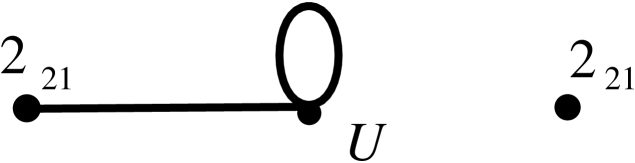
Figure 2: $n=6$. left: $\overline{G}(\overline{V},\overline{E})$, right: $G(V,E)$.

For $n=7$ the discovered adjacency component of $\overline{G}(\overline{V},\overline{E})$ has 4 vertices and that of $G(V,E)$ has two vertices (see Figure 3). The latter two vertices correspond to the Gosset 7-polytope $3_{21}$ and a polytope with 35 vertices discovered earlier by Erdahl and Rybnikov (see [ErRyb]).

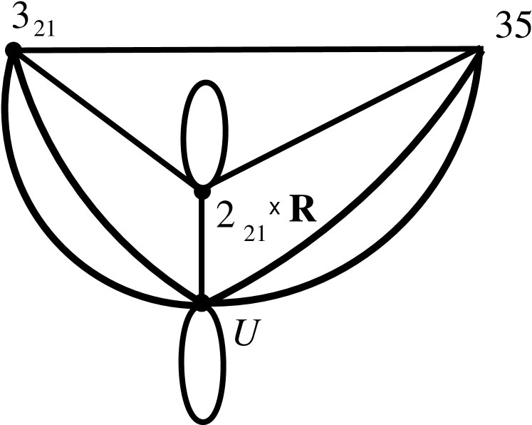
Figure 3: $n=7$. left: conjectured $\overline{G}(\overline{V},\overline{E})$, right: conjectured $G(V,E)$.

For $n=8$ we have determined an adjacency component of the restricted graph $G(V,E)$. Below is the adjacency list of the conjectured $G(V,E)$ in GAP format. Note that the graph has loops and multiple edges.

1: [1, 2]

2: [2, 16], [2, 27], [2, 8], [2, 10], [2, 22], [2, 4], [2, 5], [2, 13], [2, 7], [2, 6], [2, 3], [2, 14], [2, 12], [2, 19], [2, 9], [2, 18], [2, 8], [2, 11], [2, 15], [2, 6], [2, 11], [2, 2], [2, 17], [2, 1]

3: [3, 20], [3, 13], [3, 12], [3, 3], [3, 11], [3, 4], [3, 14], [3, 5], [3, 15], [3, 10], [3, 6], [3, 2]

4: [4, 5], [4, 6], [4, 10], [4, 22], [4, 3], [4, 2], [4, 8], [4, 14], [4, 20], [4, 19]

5: [5, 9], [5, 21], [5, 6], [5, 10], [5, 5], [5, 9], [5, 6], [5, 22], [5, 8], [5, 20], [5, 4], [5, 3], [5, 2]

6: [6, 22], [6, 10], [6, 5], [6, 4], [6, 10], [6, 3], [6, 2], [6, 9], [6, 6], [6, 5], [6, 21], [6, 8], [6, 12], [6, 15], [6, 24], [6, 6], [6, 7], [6, 11], [6, 2], [6, 15]

7: [7, 7], [7, 12], [7, 21], [7, 22], [7, 9], [7, 24], [7, 19], [7, 8], [7, 6], [7, 10], [7, 2]

8: [8, 22], [8, 2], [8, 27], [8, 8], [8, 16], [8, 8], [8, 10], [8, 20], [8, 9], [8, 6], [8, 2], [8, 5], [8, 8], [8, 4], [8, 13], [8, 12], [8, 7]

9: [9, 8], [9, 6], [9, 5], [9, 22], [9, 5], [9, 7], [9, 2], [9, 10], [9, 19], [9, 21], [9, 23], [9, 20], [9, 22]

10: [10, 6], [10, 5], [10, 15], [10, 24], [10, 10], [10, 22], [10, 9], [10, 12], [10, 21], [10, 7], [10, 10], [10, 10], [10, 3], [10, 2], [10, 20], [10, 8], [10, 4], [10, 26], [10, 6], [10, 12], [10, 13], [10, 16], [10, 16]

11: [11, 6], [11, 3], [11, 2], [11, 2]

12: [12, 10], [12, 20], [12, 3], [12, 8], [12, 10], [12, 2], [12, 7], [12, 6], [12, 21]

13: [13, 10], [13, 20], [13, 3], [13, 8], [13, 2]

14: [14, 4], [14, 18], [14, 3], [14, 2]

15: [15, 2], [15, 6], [15, 6], [15, 3], [15, 10], [15, 21]

16: [16, 8], [16, 2], [16, 27], [16, 20], [16, 10], [16, 10],

17: [17, 2]

18: [18, 19], [18, 2], [18, 14]

19: [19, 9], [19, 7], [19, 2], [19, 4], [19, 20], [19, 18], [19, 25]

20: [20, 16], [20, 22], [20, 9], [20, 5], [20, 19], [20, 4], [20, 20], [20, 12], [20, 3], [20, 13], [20, 10], [20, 8]

21: [21, 7], [21, 12], [21, 24], [21, 21], [21, 22], [21, 15], [21, 5], [21, 9], [21, 23], [21, 26], [21, 6], [21, 10]

22: [22, 22], [22, 2], [22, 8], [22, 6], [22, 27], [22, 9], [22, 7], [22, 4], [22, 5], [22, 10], [22, 9], [22, 22], [22, 21], [22, 20],

23: [23, 9], [23, 21], [23, 25]

24: [24, 6], [24, 21], [24, 7], [24, 10]

25: [25, 23], [25, 19]

26: [26, 10], [26, 21]

27: [27, 8], [27, 22], [27, 16], [27, 2]

The numbers of vertices correspond to the numbers of polytopes in [DuErRy] where a complete analysis of existing data on perfect Delaunay polyhedra for $n\leq 8$ is given.

In practice the algorithm often encounters perfect ellipsoids equivalent to the unit slab, i.e., to the set $0\leq x_{1}\leq 1$. For $n\in\{6,7,8\}$ we know that any perfect polyhedron adjacent to the unit slab is either a unit slab or the product of Gosset’s $6$-polytope $2_{21}$ and $\mathbb{R}^{n-6}$. However, for $n>6$ other unbounded perfect polyhedra appear, such as e.g. the product of $2_{21}$ and $\mathbb{R}^{2}$ for $n=8$. We are not able, at the present, to comprehensively handle all subsets $S$ with $\operatorname{\mathsf{qrank}}S=2$ for such polyhedra. That is why we cannot formally claim that our results for $n=7,8$ are complete.

4 Discussion

The new method has many advantages over the one of [Du05]:

1. Unlike the previous methods (see e.g. [Du05]), the new method uses the full symmetry group of $P$. In particular, the use of the full symmetry group of $P$ allows us to use the Recursive Adjacency Decomposition Method of [BDS07] to terminate computations. The termination problem is an important one. Previous methods did not have a satisfactory solutions to the termination problem.

2. Previous methods had to select an affine basis for each perfect Delaunay polytope. We do not know if it is possible to find an affine basis for every perfect Delaunay polytope. The method of this paper does not require this assumption.

3. Our method is no longer reduced to basic Delaunay polytopes. We know that there exist non-basic Delaunay polytopes (see [DG07]) and we cannot exclude the possibility that there exist non-basic perfect Delaunay polytopes.

4. The new method has found all presently known $8$-dimensional perfect Delaunay polytopes. The method of [Du05] run in dimension $8$ does not find some of these polytopes – they were found as sections of higher-dimensional perfect Delaunay polytopes obtained earlier by the old method; however, these sections were found by a heuristic approach without any guarantee of completeness. On the other hand, if Conjecture 1 is true, then the new algorithm has provably found all perfect Delaunay $n$-polytopes for $n\leq 8$. We expect that running the new algorithm for $n=9,10$ will uncover previously unknown perfect polytopes in these dimensions.

Our method cannot deal at present with unbounded perfect Delaunay polyhedra. When a perfect polyhedron $P$ is unbounded, but not equivalent to the unit slab, it is difficult to find all equivalence classes of its vertex subsets corresponding to the ridges of $\operatorname{E}(n)$. For this reason we cannot guarantee that our algorithm has found all perfect ellipsoids in dimensions 7 and 8.

References

- [BDS07] D. Bremner, M. Dutour Sikiric, A. Schuermann, Polyhedral representation conversion up to symmetries, http://www.arxiv.org/abs/math.MG/0702239
- [Del] B. N. Delone [Delaunay], The St. Petersburg School of Number Theory, AMS, History of Mathematics, vol. 26 (2005).
- [DL97] M. Deza, M. Laurent, (1997) Geometry of cuts and metrics. Algorithms and Combinatorics, 15. Springer-Verlag, Berlin.
- [LCVP] M. Dutour (2003), Lattice-CVP, http://www.liga.ens.fr/~dutour/CVP/index.html
- [DuPol] M. Dutour (2003), Polyhedral, http://www.liga.ens.fr/~dutour/Polyhedral/index.html
- [Du05] M. Dutour, Adjacency method for extreme Delaunay polytopes, Proceedings of “Third Voronoï Conference of the Number Theory and Spatial Tesselations”, (2005) 94–101.
- [DuErRy] M. Dutour , R. Erdahl and K. Rybnikov, Perfect Delaunay Polytopes in Low Dimensions http://www.arxiv.org/pdf/math.MG/0702136
- [Er92] R. Erdahl, A cone of inhomogeneous second-order polynomials, Discrete Comput. Geom. 8-4 (1992) 387–416.
- [Er75] R. Erdahl, A convex set of second-order inhomogeneous polynomials with applications to quantum mechanical many body theory, Mathematical Preprint #1975-40, Queen’s University, Kingston Ontario, (1975).
- [E00] R. M. Erdahl, A structure theorem for Voronoi polytopes of lattices, Talk at the sectional meeting # 957 of AMS, Toronto, September 22-24, (2000).
- [ErRyb] R. Erdahl and K. Rybnikov, Supertopes, http://faculty.uml.edu/krybnikov/
- [DG07] M. Dutour and V. Grishukhin, How to compute the rank of a Delaunay polytope, European Journal of Combinatorics, in press.
- [McKay] B. McKay, The nauty program, http://cs.anu.edu.au/people/bdm/nauty/
- [DER07] M. Dutour, R. Erdahl, K. Rybnikov, Perfect Delaunay Polytopes in Low Dimensions, http://www.arxiv.org/abs/math.MG/0702136
- [CK70] D.R. Chand and S.S. Kapur, An algorithm for convex polytopes, Journal of the ACM 17 (1970), 78–86.
- [RB79] S. S. Ryshkov, E. P. Baranovskii, Classical methods in the theory of lattice packings, Russian Mathematical Surveys 34, (1979).
- [Ven40] B. Wenkov [B. A. Venkov], Über die Reduction positiver quadratischer Formen. (Russian) Bull. Acad. Sci. URSS. S r. Math. [Izvestia Akad. Nauk SSSR] 4, (1940). 37–52.
- [VorI08] G. F. Voronoi, Nouvelles applications des paramèters continus à la théorie des formes quadratiques, Prèmier memoire, J. Reine Angew. Math., 133 (1908), 97–178.
- [VorII08-09] G. F. Voronoi, Nouvelles applications des paramèters continus à la théorie des formes quadratiques, Deuxième memoire, J. Reine Angew. Math., 134 (1908), 198-287, 136 (1909), 67–178.
- [VorCol] G. F. Voronoi, Sobranie sočineniĭ v treh tomah. (Russian) [Collected works in three volumes.] Izdatel’stvo Akademii Nauk Ukrainskoĭ. SSR, Kiev. (1952, 1953); Vol. I, 1952, 399 pp.; Vol. II, 1952; 391 pp.; Vol. III, 1953, 306 pp.