Lifetime difference in $D^{0}$-${\overline{D}}^{0}$ mixing within R-parity-violating SUSY

Abstract

We re-examine constraints from the recent evidence for observation of the lifetime difference in $D^{0}-\overline{D}{}^{0}$ mixing on the parameters of supersymmetric models with $R$-parity violation (RPV). We find that RPV SUSY can give large negative contribution to the lifetime difference. We also discuss the importance of the choice of weak or mass basis when placing the constraints on RPV-violating couplings from flavor mixing experiments.

I Introduction

Meson-antimeson mixing is an important vehicle for indirect studies of New Physics (NP). Due to the absence of tree-level flavor-changing neutral current transitions in the Standard Model (SM), it can only occur via quantum effects associated with the SM and NP particles. In fact, the existence of both charm and top quark were inferred from the kaon and beauty mixing amplitudes 48 . The estimates of masses of those particles were later found to be in agreement with direct observations. This motivates indirect searches for NP particles in a meson-antimeson mixing.

Recently, there has been a considerable interest in the only available meson-antimeson mixing in the up-quark sector, the $D^{0}-\overline{D}{}^{0}$ mixing 36 . The fact that the search is indirect and complimentary to existing constraints from the bottom-quark sector actually provides parameter space constraints for a large variety of NP models 23 ; 6 .

A flurry of recent experimental activity in that field led to the observation of $D^{0}-\overline{D}{}^{0}$ mixing from several different experiments such as BaBar 34 , Belle 35 and CDF CDFmix . These results have been combined by the Flavor Averaging Group (HFAG) 38 to yield

$$y^{exp}_{\rm D}=(6.6\pm 2.1)\cdot 10^{-3}$$ (1.1)

$$x^{exp}_{\rm D}=8.7^{+3.0}_{-3.4}\cdot 10^{-3},$$ (1.2)

where $x_{\rm D}$ and $y_{\rm D}$ are defined as

$$x_{\rm D}\equiv{\Delta M_{\rm D}\over\Gamma_{\rm D}},\qquad{\rm and}\qquad y_{\rm D}\equiv{\Delta\Gamma_{\rm D}\over 2\Gamma_{\rm D}}\ \ ,$$ (1.3)

$\Gamma_{\rm D}$ is the average width of the two neutral $D$ meson mass eigenstates, and $\Delta M_{\rm D}$, $\Delta\Gamma_{\rm D}$ are the mass and width differences of the neutral D-meson mass eigenstates. In the limit of CP-conservation, $\Delta\Gamma_{D}\equiv\Gamma_{+}-\Gamma_{-}$, where ”+” and ”-” are CP-even and CP-odd D-meson eigenstates respectively.

One can also write $y_{D}$ as an absorptive part of the $D^{0}-\overline{D}{}^{0}$ mixing matrix Petrov:2003un ,

$$y_{D}=\frac{1}{\Gamma_{\rm D}}\sum_{n}\rho_{n}\langle\overline{D}^{0}|{\cal H}_{w}^{\Delta C=1}|n\rangle\langle n|{\cal H}_{w}^{\Delta C=1}|D^{0}\rangle,$$ (1.4)

where $\rho_{n}$ is a phase space function that corresponds to a charmless intermediate state $n$. This relation shows that $\Delta\Gamma_{\rm D}$ is driven by transitions $D^{0},{\overline{D}}^{0}\rightarrow n$, i.e. physics of the $\Delta C=1$ sector.

Eqs. (1.1) and (1.2) imply one-sigma window for the HFAG values of $x_{D}$ and $y_{\rm D}$,

$$5.3\cdot 10^{-3}<x_{D}<11.7\cdot 10^{-3}\qquad{\rm(one-sigma\ window)}\ \$$ (1.5)

$$4.5\cdot 10^{-3}<y_{\rm D}<8.7\cdot 10^{-3}\qquad\ \ {\rm(one-sigma\ window)}\ \$$ (1.6)

In principle, these results can be used to constrain parameters of NP models with the anticipated improved accuracy for the future D-mixing measurements. In reality, those results can only provide the ballpark estimate to be used for constraining NP models. The reason is that the SM estimate for the parameters $x_{\rm D}$ and $y_{\rm D}$ is rather uncertain, as it is dominated by long-distance QCD effects 29 -49 . It was nevertheless shown that even this estimate provides rather stringent constraints on the NP parameter space for many models affecting the mass difference $x_{\rm D}$ 23 , 41 -46 .

It was recently shown 6 that $D^{0}-\overline{D}{}^{0}$ mixing is a rather unique system, where $y_{\rm D}$ can also be used to constrain the models of New Physics. This stems from the fact that there is a well-defined theoretical limit (the flavor $SU(3)$-limit) where the SM contribution vanishes and the lifetime difference is dominated by the NP $\Delta C=1$ contributions. In real world, flavor $SU(3)$ is, of course, broken, so the SM contribution is proportional to a (second) power of $m_{s}/\Lambda$, which is a rather small number. If the NP contribution to $y_{\rm D}$ is non-zero in the flavor $SU(3)$-limit, it can provide a large contribution to the mixing amplitude.

To see this, consider a $D^{0}$ decay amplitude which includes a small NP contribution, $A[D^{0}\rightarrow n]=A_{n}^{\rm(SM)}+A_{n}^{\rm(NP)}$. Experimental data for D-meson decays are known to be in a decent agreement with the SM estimates 47 ; 28 . Thus, $A_{n}^{\rm(NP)}$ should be smaller than (in sum) the current theoretical and experimental uncertainties in predictions for these decays.

One may rewrite equation (1.4) in the form (neglecting the effects of CP-violation)

$$y_{D} = \sum_{n}\frac{\rho_{n}}{\Gamma_{\rm D}}A_{n}^{\rm(SM)}\bar{A}_{n}^{\rm(SM)}+2\sum_{n}\frac{\rho_{n}}{\Gamma_{\rm D}}A_{n}^{\rm(NP)}\bar{A}_{n}^{\rm(SM)}+\sum_{n}\frac{\rho_{n}}{\Gamma_{\rm D}}A_{n}^{\rm(NP)}\bar{A}_{n}^{\rm(NP)}\ \ .$$ (1.7)

The first term in this equation corresponds to the SM contribution, which vanishes in the $SU(3)$ limit. In ref. 6 the last term in (1.7) has been neglected, thus the NP contribution to $y_{\rm D}$ comes there solely from the second term, due to interference of $A_{n}^{\rm(SM)}$ and $A_{n}^{\rm(NP)}$. While this contribution is in general non-zero in the flavor $SU(3)$ limit, in a large class of (popular) models it actually is 6 ; 37 . Then, in this limit, $y_{\rm D}$ is completely dominated by pure $A_{n}^{\rm(NP)}$ contribution given by the last term in eq. (1.7)! It is clear that the last term in equation (1.7) needs more detailed and careful studies, at least within some of the NP models.

Indeed, in reality, flavor $SU(3)$ symmetry is broken, so the first term in Eq. (1.7) is not zero. It has been argued 29 that in fact the SM $SU(3)$-violating contributions could be at a percent level, dominating the experimental result. The SM predictions of $y_{D}$, stemming from evaluations of long-distance hadronic contributions, are rather uncertain. While this precludes us from placing explicit constraints on parameters of NP models, it has been argued that, even in this situation, an upper bound on the NP contributions can be placed 23 by displaying the NP contribution only, i.e. as if there were no SM contribution at all. This procedure is similar to what was traditionally done in the studies of NP contributions to $K^{0}-\overline{K}^{0}$ mixing, so we shall employ it here too.

The purpose of this paper is to revisit the problem of the NP contribution to $y_{\rm D}$ and provide constraints on R-parity-violating supersymmetric (SUSY) models as a primary example. It has been recently argued in 17 that within /R- SUSY models, new physics contribution to $y_{\rm D}$ is rather small, mainly because of stringent constraints on the relevant pair products of RPV coupling constants. However, this result has been derived neglecting the transformation of these couplings from the weak isospin basis to the quark mass basis. This approach seems to be quite reasonable for the scenarios with the baryonic number violation. However, in the scenarios with the leptonic number violation, transformation of the RPV couplings from the weak eigenbasis to the quark mass eigenbasis turns to be crucial, when applying the existing phenomenological constraints on these couplings.

We show in the present paper that within R-parity-breaking supersymmetric models with the leptonic number violation, new physics contribution to the lifetime difference in $D^{0}-\overline{D}{}^{0}$ mixing may be large, due to the last term in eq. (1.7). When being large, it is negative (if neglecting CP-violation), i.e. opposite in sign to what is implied by the recent experimental evidence for $D^{0}-\overline{D}{}^{0}$ mixing.

The paper is organized as follows. In Section 2 we discuss the R-parity violating interactions that, in particular, contribute to $D^{0}-\overline{D}{}^{0}$ lifetime difference. We confront the form of these interactions in the weak isospin basis to that in the quark mass basis, emphasizing the important differences. In Section 3 we re-derive formulae for the RPV SUSY contribution to $y_{\rm D}$. Unlike ref. 17 , transformation of the RPV coupling constants from the weak to the quark mass eigenbasis is taken into account. Also the behavior of different /R- SUSY contributions in the limit of the flavor SU(3) symmetry is discussed in details. In Section 4 we examine the existing phenomenological constraints on the RPV coupling constants. The importance of taking into account the transformation of these couplings from the weak to the mass eigenbasis is emphasized again. We present our numerical results in Section 5. We conclude in Section 6. Appendices contain some details of derivation of bounds on the pair products of RPV couplings, relevant for our analysis.

II R-Parity Breaking Interactions: Weak vs Mass Eigenbases

We consider a general low-energy supersymmetric scenario with no assumptions made on a SUSY breaking mechanism at the unification scales $(\sim~{}(10^{16}~{}-~{}10^{18})GeV)$. The most general Yukawa superpotential for an explicitly broken R-parity supersymmetric theory is given by

$$W_{/{R}}=\sum_{i,j,k}\left[\frac{1}{2}\lambda_{ijk}L_{i}L_{j}E^{c}_{k}+\lambda^{\prime}_{ijk}L_{i}Q_{j}D^{c}_{k}+\frac{1}{2}\lambda^{\prime\prime}_{ijk}U^{c}_{i}D^{c}_{j}D^{c}_{k}\right]$$ (2.1)

where $L_{i}$, $Q_{j}$ are $SU(2)_{L}$ weak isodoublet lepton and quark superfields, respectively; $E_{i}^{c}$, $U_{i}^{c}$, $D_{i}^{c}$ are SU(2) singlet charged lepton, up- and down-quark superfields, respectively; $\lambda_{ijk}$ and $\lambda^{\prime}_{ijk}$ are lepton number violating Yukawa couplings, and $\lambda^{\prime\prime}_{ijk}$ is a baryon number violating Yukawa coupling; $\lambda_{ijk}=-\lambda_{jik}$, $\lambda^{\prime\prime}_{ijk}=-\lambda^{\prime\prime}_{ikj}$. To avoid rapid proton decay, we assume that $\lambda^{\prime\prime}_{ijk}=0$ and work with a lepton number violating /R- SUSY model.

For meson-to-antimeson oscillation processes, to the lowest order in the perturbation theory, only the second term of (2.1) is of the importance. The relevant R-parity breaking part of the Lagrangian is the following:

$${\cal L}_{/{}R}=\sum_{i,j,k}\lambda^{\prime}_{ijk}\Biggl{[}-\widetilde{e}_{i_{L}}\bar{d}_{k_{R}}^{w}u_{j_{L}}^{w}-\widetilde{u}_{j_{L}}^{w}\bar{d}_{k_{R}}^{w}e_{i_{L}}-\widetilde{d}^{w^{*}}_{k_{R}}\bar{e}_{i_{R}}^{c}u_{j_{L}}^{w}+\widetilde{\nu}_{i_{L}}\bar{d}_{k_{R}}^{w}d_{j_{L}}^{w}+$$

$$+\widetilde{d}_{j_{L}}^{w}\bar{d}_{k_{R}}^{w}\nu_{i_{L}}+\widetilde{d}^{w^{*}}_{k_{R}}\bar{\nu}_{i_{R}}^{c}d_{j_{L}}^{w}\Biggr{]}+h.c.$$ (2.2)

The superscript $w$ indicates that the quark and squark states in (2.2) are weak isospin eigenstates. The weak and mass quark eigenstates are related by the unitary transformations (we assume that left- and right-chiral quarks have the same transformation matrices):

$$u^{w}_{j}=S_{u_{jn}}u_{n},\hskip 14.22636ptd^{w}_{k}=S_{d_{km}}d_{m}$$ (2.3)

where

$$\sum_{j,j^{\prime}}S^{*}_{u_{j^{\prime}n^{\prime}}}Y_{u_{j^{\prime}j}}S_{u_{jn}}=\delta_{nn^{\prime}}h_{u_{n}},\hskip 14.22636pt\sum_{k,k^{\prime}}S^{*}_{d_{k^{\prime}m^{\prime}}}Y_{d_{k^{\prime}k}}S_{d_{km}}=\delta_{mm^{\prime}}h_{d_{m}}$$ (2.4)

and

$$\sum_{k}S^{*}_{u_{kj}}S_{d_{kn}}=V_{jn}$$ (2.5)

In (2.4) $Y_{u}$, $Y_{d}$ are quark-Higgs-quark R-parity conserving Yukawa couplings in the weak isospin basis and $h_{u}$, $h_{d}$ are these couplings in the quark mass eigenbasis. In (2.5), $V_{jn}$ stands as usually for the (Standard Model) CKM matrix.

Generally speaking, squark transformation matrices from the weak to the mass eigenstates are different from those for quarks. Nevertheless, we choose for squarks to be rotated by the same matrices $S_{u}$ and $S_{d}$ that make quark mass matrices diagonal, i.e.

$$\widetilde{u}^{w}_{j_{L}}=S_{u_{jn}}\widetilde{u}_{n_{L}},\hskip 14.22636pt\widetilde{u}^{w}_{j_{R}}=S_{u_{jn}}\widetilde{u}_{n_{R}}$$

$$\widetilde{d}^{w}_{k_{L}}=S_{d_{km}}\widetilde{d}_{m_{L}},\hskip 14.22636pt\widetilde{d}^{w}_{k_{R}}=S_{d_{km}}\widetilde{d}_{m_{R}}$$ (2.6)

This is a super-CKM basis, in which the squark mass matrices are non-diagonal and result in mass insertions that change the squark flavors 30 -33 . This source of flavor violation is very important in the pure MSSM sector. In particular, it plays crucial role in examining the MSSM contribution to $D^{0}-\bar{D}^{0}$ mass difference 23 .

In the R-parity breaking part of SUSY Lagrangian, flavor changing neutral currents are present a priori. In order to simplify our analysis, we put all the squark masses to be nearly equal. Then the squark mass matrix is proportional to the identity matrix, i.e. it is diagonal in any basis.

Using (2.3), (2.5) and (2.6), one may rewrite (2.2) as

$${\cal L}_{/{}R}=-\sum_{i,j,k,m,n,r}\lambda^{\prime}_{ijk}S^{*}_{d_{km}}S_{d_{jn}}V_{rn}^{*}\left[\widetilde{e}_{i_{L}}\bar{d}_{m_{R}}u_{r_{L}}+\widetilde{u}_{r_{L}}\bar{d}_{m_{R}}e_{i_{L}}+\widetilde{d}^{*}_{m_{R}}\bar{e}_{i_{R}}^{c}u_{r_{L}}\right]+$$

$$+\sum_{i,j,k,m,n}\lambda^{\prime}_{ijk}S_{d_{km}}^{*}S_{d_{jn}}\left[\widetilde{\nu}_{i_{L}}\bar{d}_{m_{R}}d_{n_{L}}+\widetilde{d}_{n_{L}}\bar{d}_{m_{R}}\nu_{i_{L}}+\widetilde{d}^{*}_{m_{R}}\bar{\nu}_{i_{R}}^{c}d_{n_{L}}\right]+h.c.$$ (2.7)

At this point one may redefine, without loss of generality, the couplings $\lambda^{\prime}$ as

$$\lambda^{\prime}_{ijk}S^{*}_{d_{km}}S_{d_{jn}}\rightarrow\lambda^{\prime}_{inm}$$ (2.8)

This is also equivalent to choosing the weak and mass eigenbases for down-quarks being the same, while for up-quarks they are related by the CKM matrix.

Defining $\widetilde{\lambda}^{\prime}_{irm}\ =\ V^{*}_{rn}\ \lambda^{\prime}_{inm}$ and renaming the summation indices, we rewrite (2.7) as

$${\cal L}_{/{}R}=-\sum_{i,j,k}\widetilde{\lambda}^{\prime}_{ijk}\left[\widetilde{e}_{i_{L}}\bar{d}_{k_{R}}u_{j_{L}}+\widetilde{u}_{j_{L}}\bar{d}_{k_{R}}e_{i_{L}}+\widetilde{d}^{*}_{k_{R}}\bar{e}_{i_{R}}^{c}u_{j_{L}}\right]+$$

$$+\sum_{i,j,k}\lambda^{\prime}_{ijk}\left[\widetilde{\nu}_{i_{L}}\bar{d}_{k_{R}}d_{j_{L}}+\widetilde{d}_{j_{L}}\bar{d}_{k_{R}}\nu_{i_{L}}+\widetilde{d}^{*}_{k_{R}}\bar{\nu}_{i_{R}}^{c}d_{j_{L}}\right]+h.c.$$ (2.9)

As it follows from (2.9), (s)down-down-(s)neutrino vertices have the weak eigenbasis couplings $\lambda^{\prime}$, while charged (s)lepton-(s)down-(s)up vertices have the up quark mass eigenbasis couplings $\tilde{\lambda}^{\prime}$.

Very often in the literature (see e.g. 6 , 17 , 2 -5 ) one neglects the difference between $\lambda^{\prime}$ and $\widetilde{\lambda}^{\prime}$, based on the fact that diagonal elements of the CKM matrix dominate over non-diagonal ones, i.e.

$$V_{jn}=\delta_{jn}+O(\lambda)\qquad\mbox{so}\qquad\widetilde{\lambda}_{ijk}\approx\lambda^{\prime}_{ijk}+O(\lambda)$$ (2.10)

where $\lambda=\sin\theta_{c}\sim 0.2$, with $\theta_{c}$ being the Cabibbo angle.

Notice that relation Eq. (2.10) is valid if only there is no hierarchy in couplings $\lambda^{\prime}$. On the other hand, the existing strong bounds on pair products $\lambda^{\prime}\times\lambda^{\prime}$ (or $\widetilde{\lambda}^{\prime}\times\widetilde{\lambda^{\prime}}$) 1 ; 2 ; 3 and relatively loose bounds on individual couplings $\lambda^{\prime}$ 1 suggest that such a hierarchy may exist. As we will see in Section 4, pair products $\widetilde{\lambda}^{\prime}\times\widetilde{\lambda^{\prime}}$ may be orders of magnitude greater than corresponding products $\lambda^{\prime}\times\lambda^{\prime}$.

To the end of this section, we explicitly write down the terms of the R-parity breaking part of the Lagrangian that contribute to $D^{0}-\bar{D}^{0}$ lifetime difference:

$${\cal L}{{}^{D^{0}-\bar{D}^{0}}}=-\sum_{i}\Biggl{[}\widetilde{\lambda}^{\prime}_{i21}\tilde{e}_{i_{L}}\bar{d}\left(\frac{1-\gamma_{5}}{2}\right)c+\widetilde{\lambda}_{i22}^{\prime}\tilde{e}_{i_{L}}\bar{s}\left(\frac{1-\gamma_{5}}{2}\right)c+$$

$$+\widetilde{\lambda}_{i11}^{\prime*}\tilde{e}_{i_{L}}^{*}\bar{u}\left(\frac{1+\gamma_{5}}{2}\right)d+\widetilde{\lambda}_{i12}^{\prime*}\tilde{e}_{i_{L}}^{*}\bar{u}\left(\frac{1+\gamma_{5}}{2}\right)s\Biggr{]}-$$

$$-\sum_{k}\Biggl{[}\widetilde{\lambda}^{\prime}_{12k}\tilde{d}^{*}_{k_{R}}\bar{e}^{c}\left(\frac{1-\gamma_{5}}{2}\right)c+\widetilde{\lambda}^{\prime}_{22k}\tilde{d}^{*}_{k_{R}}\ \bar{\mu}^{c}\left(\frac{1-\gamma_{5}}{2}\right)c+$$

$$+\widetilde{\lambda}^{\prime*}_{11k}\tilde{d}_{k_{R}}\bar{u}\left(\frac{1+\gamma_{5}}{2}\right)e^{c}+\widetilde{\lambda}^{\prime*}_{21k}\tilde{d}_{k_{R}}\bar{u}\left(\frac{1+\gamma_{5}}{2}\right)\mu^{c}\Biggr{]}$$ (2.11)

In the next section we will integrate out heavy degrees of freedom in (2.11), thus finding /R-SUSY part of $\Delta C=1$ effective Hamiltonian. Then we will compute R-parity breaking SUSY contribution to $\Delta\Gamma_{D}$.

III $D^{0}-\bar{D}^{0}$ Lifetime Difference

Assuming CP-conservation, the normalized $D^{0}-\bar{D}^{0}$ lifetime difference is given by

$$y_{D}=\frac{1}{2m_{D}\Gamma_{D}}Im\left[\langle\bar{D}^{0}|i\int d^{4}x\ T\left\{H_{W}^{\Delta C=1}(x)H_{W}^{\Delta C=1}(0)\right\}|D^{0}\rangle\right],$$ (3.1)

where $H_{W}^{\Delta C=1}$ is an effective Hamiltonian including both SM and NP parts. To the lowest order in the perturbation theory, /R-SUSY contribution to $D^{0}-\bar{D}^{0}$ mixing comes from the one-loop graphs with

• $W^{\pm}$ boson, charged slepton and two down-type quarks (Fig. 1a);

• two charged sleptons and two down-type quarks (Fig. 2a);

• two down-type squarks and two charged leptons (Fig. 3a) .

Within the low-energy effective theory, $D^{0}-\bar{D}^{0}$ lifetime difference occurs as a result of a bi-local transition with two $\Delta C=1$ effective vertices. The relevant low-energy diagrams in Fig.’s 1b) - 3b) are derived by integrating out of heavy $W^{\pm}$ boson, charged slepton and down-type squark degrees of freedom.

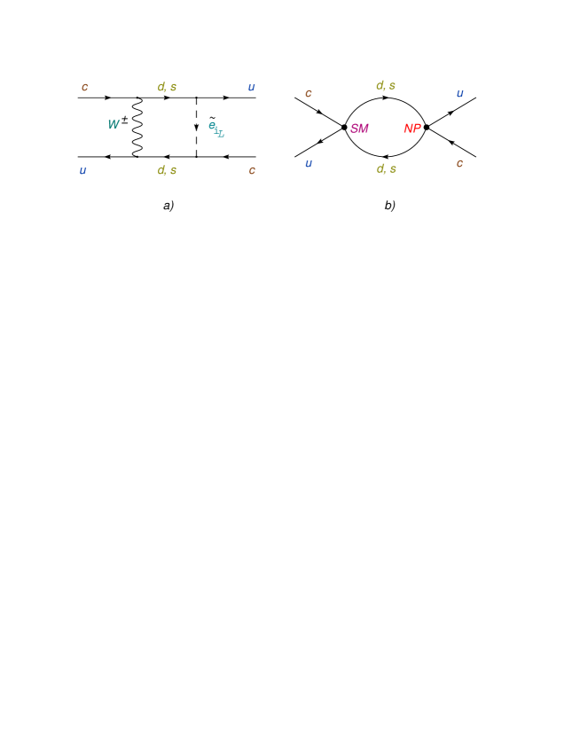
Figure 1: $D^{0}-\bar{D}^{0}$ mixing diagrams with R-parity breaking interactions: a) within the full electroweak theory; b) within the low-energy effective theory. In these diagrams, $D^{0}-\bar{D}^{0}$ oscillations occur via two subsequent $\Delta C=1$ transitions with the exchange of $W^{\pm}$ boson and a charged ”left” slepton, i=1,2,3.

For R-parity-violating SUSY models one can therefore write

$$H_{W}^{\Delta C=1}=H_{W_{SM}}^{\Delta C=1}+H_{W_{\tilde{\ell}}}^{\Delta C=1}+H_{W_{\tilde{q}}}^{\Delta C=1}$$ (3.2)

The first term in the r.h.s of (3.2) is the Standard Model contribution, whereas the second term comes from $\Delta C=1$ transitions with a slepton exchange and the last term comes from $\Delta C=1$ transitions with a squark exchange. The Standard model part of $\Delta C=1$ effective Hamiltonian is given by

$$H_{W_{SM}}^{\Delta C=1} = \frac{G_{F}}{\sqrt{2}}\Biggl{[}C_{1}(\mu_{c})\ \delta^{a_{1}a_{4}}\ \delta^{a_{3}a_{2}}+C_{2}(\mu_{c})\ \delta^{a_{1}a_{2}}\ \delta^{a_{3}a_{4}}\Biggr{]}$$ (3.3)

$$\times \sum_{q_{1},\ q_{2}}V_{uq_{1}}V^{*}_{cq_{2}}\ \bar{u}^{a_{1}}(x)\gamma^{\mu}(1-\gamma_{5})q_{1}^{a_{2}}(x)\ \bar{q}_{2}^{a_{3}}(x)\gamma_{\mu}(1-\gamma_{5})c^{a_{4}}(x)$$

where $q_{1}=s,d$, $q_{2}=s,d$, $a_{i}$ are the color indices, and $C_{1}$ and $C_{2}$ are the operator Wilson coefficients. The Wilson coefficients are to be evaluated at a low-energy scale $\mu_{c}$, which we choose here as $\mu_{c}=m_{c}$.

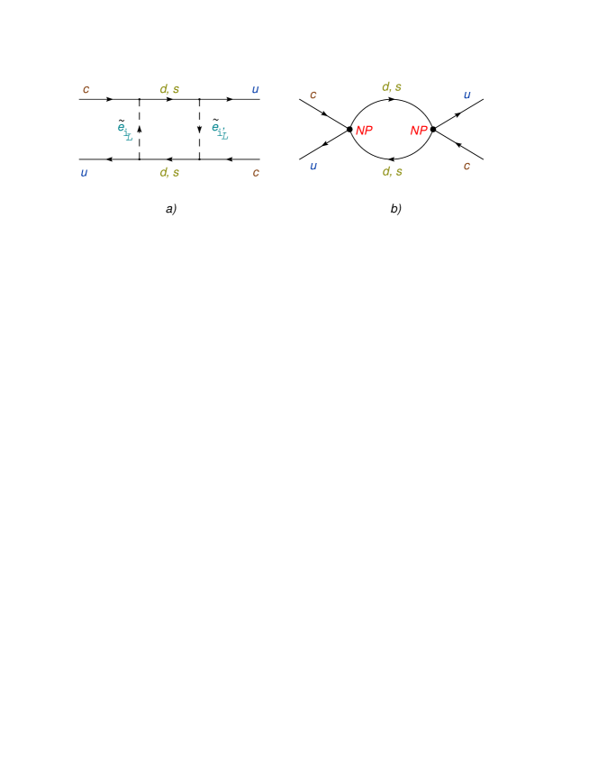
Figure 2: Same as in Fig. 1, however both of $\Delta C=1$ transitions are due to a charged slepton exchange now, $i=1,2,3$, $i^{\prime}=1,2,3$. Both of the effective $\Delta C=1$ vertices are NP vertices.

To simplify the following calculations, let us assume that all the sleptons and all squarks are nearly degenerate, i.e.

$$m_{\tilde{e}_{i}}=m_{\tilde{\nu}_{i}}=m_{\tilde{\ell}},\qquad\mbox{and}\qquad m_{\tilde{d}_{k}}=m_{\tilde{u}_{k}}=m_{\tilde{q}}.$$ (3.4)

With this assumption, the low energy effective Hamiltonian for the R-parity-violating interactions are given by

$$H_{W_{\tilde{\ell}}}^{\Delta C=1} = -\Biggl{[}\widetilde{C}_{1}(\mu_{c})\ \delta^{a_{1}a_{4}}\ \delta^{a_{3}a_{2}}+\widetilde{C}_{2}(\mu_{c})\ \delta^{a_{1}a_{2}}\ \delta^{a_{3}a_{4}}\Biggr{]}$$ (3.5)

$$\times \sum_{q_{1},\ q_{2}}\frac{\lambda_{q_{1}q_{2}}}{4m_{\tilde{\ell}}^{2}}\ \bar{u}^{a_{1}}(x)(1+\gamma_{5})q_{1}^{a_{2}}(x)\ \bar{q}_{2}^{a_{3}}(x)(1-\gamma_{5})c^{a_{4}}(x),$$

and

$$H_{W_{\tilde{q}}}^{\Delta C=1}=-\sum_{\ell_{1},\ \ell_{2}}\frac{\lambda_{\ell_{1}\ell_{2}}}{4m_{\tilde{q}}^{2}}\ \bar{u}^{a}(x)(1+\gamma_{5})\ell_{1}^{c}(x)\ \bar{\ell}_{2}^{c}(x)(1-\gamma_{5})c^{a}(x)$$ (3.6)

where $q_{1}=s,d$, $q_{2}=s,d$, $\ell_{1}=e,\mu$, and $\ell_{2}=e,\mu$. The superscript ${}^{\prime\prime}c^{\prime\prime}$ stands for charge conjugation. Also,

$$\lambda_{q_{1}q_{2}}\ \equiv\ \sum_{i}\ \widetilde{\lambda}^{\prime*}_{i1q_{1}}\ \widetilde{\lambda}^{\prime}_{i2q_{2}}\qquad\mbox{and}\qquad\lambda_{\ell_{1}\ell_{2}}\ \equiv\ \sum_{k}\ \widetilde{\lambda}^{\prime*}_{\ell_{1}1k}\ \widetilde{\lambda}^{\prime}_{\ell_{2}2k}$$ (3.7)

We assume that $\lambda_{q_{1}q_{2}}$ and $\lambda_{\ell_{1},\ell_{2}}$ are real.

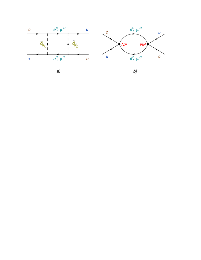
Figure 3: Same as in Fig.’s 1, 2, however both of $\Delta C=1$ transitions occur due to exchange of down-type squarks now, $k=1,2,3$, $k^{\prime}=1,2,3$. Subsequently the intermediate charmless states are charged (anti)lepton states.

The insertions of Hamiltonians of eqs. (3.3), (3.5), and (3.6) can lead to the lifetime difference in $D^{0}-\overline{D}{}^{0}$ system. Let us write it as

$$y_{D}=y_{SM}+y_{SM,NP}+y_{\tilde{\ell}\tilde{\ell}}+y_{\tilde{q}\tilde{q}},$$ (3.8)

where

$$y_{SM,NP}=\frac{1}{2m_{D}\Gamma_{D}}\ Im\Biggl{[}\langle\bar{D}^{0}|i\int d^{4}x\ T\Biggl{\{}H_{W_{SM}}^{\Delta C=1}(x)H_{W_{\tilde{\ell}}}^{\Delta C=1}(0)+$$

$$+H_{W_{\tilde{\ell}}}^{\Delta C=1}(x)H_{W_{SM}}^{\Delta C=1}(0)\Biggr{\}}|D^{0}\rangle\Biggr{]}$$ (3.9)

is the term coming form the interference of the SM and NP contributions to $H_{W}^{\Delta C=1}$, and

$$y_{\tilde{\ell}\tilde{\ell}}=\frac{1}{2m_{D}\Gamma_{D}}\ Im\Biggl{[}\langle\bar{D}^{0}|i\int d^{4}x\ T\Biggl{\{}H_{W_{\tilde{\ell}}}^{\Delta C=1}(x)H_{W_{\tilde{\ell}}}^{\Delta C=1}(0)\Biggr{\}}|D^{0}\rangle\Biggr{]},$$ (3.10)

$$y_{\tilde{q}\tilde{q}}=\frac{1}{2m_{D}\Gamma_{D}}\ Im\Biggl{[}\langle\bar{D}^{0}|i\int d^{4}x\ T\Biggl{\{}H_{W_{\tilde{q}}}^{\Delta C=1}(x)H_{W_{\tilde{q}}}^{\Delta C=1}(0)\Biggr{\}}|D^{0}\rangle\Biggr{]}$$ (3.11)

are coming from two insertions of the NP vertices.

It might seem unreasonable to include double insertions of the NP Hamiltonian to compute $y_{D}$, as each insertion generates a contribution that is suppressed by some NP scale $M_{NP}$, which in general is greater than the electroweak scale set here by $M_{W}$. Yet, as the Standard Model contribution is zero in the flavor SU(3) limit (i.e. suppressed by powers of strange quark mass), New Physics contributions can be large 6 . Also, as can be seen from refs. 6 and 17 , $y_{SM,NP}$ resulting from the single insertion of the NP Hamiltonian is forbidden in the $SU(3)$ flavor symmetry limit. Thus, double insertion of the NP Hamiltonian can be important, especially if this contribution does not vanish in the $SU(3)$ limit! This construction can give numerically large contribution to $y_{D}$ if $\left(M_{W}/M_{NP}\right)^{2}>\left(m_{s}/m_{c}\right)^{2}$.

Note that contribution to $\Delta\Gamma_{D}$ is nonzero if the intermediate states are the on-mass-shell real physical states. It is therefore easy to see from the energy-momentum conservation that diagrams like those in Fig.’s 1-3 but with b-quarks, $\tau\tau$, $\tau\mu$ pairs running a loop, are irrelevant for our analysis. While the diagrams with a $\tau e$ pair running in a loop do give nonzero contribution to $\Delta\Gamma_{D}$, their contributions are suppressed by the available phase space. Thus, we shall not consider them too.

It is known that correlation function in (3.1) (as well as those in (3.9)-(3.11)) may be presented as a sum of local $\Delta C=2$ operators, which corresponds to $1/m_{c}$ power expansion of (3.1) (or (3.9) - (3.11)). Here we are interested in the lowest order terms in this expansion. Keeping only the leading terms in $x_{s}\equiv m_{s}^{2}/m_{c}^{2}$ and $x_{d}\equiv m_{d}^{2}/m_{c}^{2}$, we get

$$y_{SM,NP}=-\frac{G_{F}}{\sqrt{2}}\ \frac{\left(K_{1}+K_{2}\right)}{4\pi m_{D}\Gamma_{D}}\ \left(\frac{m_{c}^{2}}{m_{\tilde{\ell}}^{2}}\right)\Biggl{[}\lambda_{sd}\sqrt{x_{s}x_{d}}\ +$$

$$+\ \lambda\left(\lambda_{ss}x_{s}-\lambda_{dd}x_{d}\right)-\lambda^{2}\lambda_{ds}\sqrt{x_{s}x_{d}}\ \Biggr{]}\langle Q\rangle$$ (3.12)

and

$$y_{\tilde{\ell}\tilde{\ell}}=\frac{m_{c}^{2}\left(\lambda_{ss}^{2}+\lambda_{dd}^{2}+2\lambda_{sd}\lambda_{ds}\right)}{192\pi m_{D}\Gamma_{D}m_{\tilde{\ell}}^{4}}\ \Biggl{\{}-\left[\frac{\widetilde{K}_{2}}{2}+\widetilde{K}_{1}\right]\langle Q\rangle+$$

$$+\ \left[\widetilde{K}_{2}-\widetilde{K}_{1}\right]\langle Q_{S}\rangle\Biggr{\}}$$ (3.13)

where $\lambda=\sin{\theta_{C}}$ is the Wolfenstein parameter, and

$$\langle Q\rangle\equiv\langle\bar{D}^{0}|\ \bar{u}^{a_{1}}(0)\gamma^{\mu}\left(\frac{1-\gamma_{5}}{2}\right)c^{a_{1}}(0)\ \bar{u}^{a_{2}}(0)\gamma_{\mu}\left(\frac{1-\gamma_{5}}{2}\right)c^{a_{2}}(0)\ |D^{0}\rangle$$ (3.14)

$$\langle Q_{S}\rangle\equiv\langle\bar{D}^{0}|\ \bar{u}^{a_{1}}(0)\left(\frac{1+\gamma_{5}}{2}\right)c^{a_{1}}(0)\ \bar{u}^{a_{2}}(0)\left(\frac{1+\gamma_{5}}{2}\right)\ c^{a_{2}}(0)\ |D^{0}\rangle$$ (3.15)

are the matrix elements of the effective low energy $\Delta C=2$ operators and

$$K_{1}\ =\ 3\ C_{1}\ \widetilde{C}_{1}+C_{1}\ \widetilde{C}_{2}+C_{2}\ \widetilde{C}_{1},\hskip 14.22636ptK_{2}\ =\ C_{2}\ \widetilde{C}_{2}$$ (3.16)

$$\widetilde{K}_{1}\ =\ 3\ \widetilde{C}_{1}^{2}+2\ \widetilde{C}_{1}\ \widetilde{C}_{2},\hskip 65.44142pt\widetilde{K}_{2}\ =\ \widetilde{C}_{2}^{2}$$ (3.17)

are the Wilson coefficients. It is important to stress that $y_{SM,NP}$, just like a Standard Model contribution, vanishes in the limit of exact flavor $SU(3)$ symmetry - it is proportional to light quark masses via $x_{s}$, $x_{d}$ and $\sqrt{x_{s}x_{d}}$. On the contrary, $y_{\tilde{\ell}\tilde{\ell}}$ is nonzero even in the limit of exact flavor $SU(3)$ symmetry! Therefore, as we shall see in Section 5, $y_{\tilde{\ell}\tilde{\ell}}$ dominates over $y_{SM,NP}$ if R-parity breaking coupling products $\lambda_{ss}$ and/or $\lambda_{dd}$ approach their boundaries. In other words, contribution of diagrams in Fig. 2 with both of $\Delta C=1$ vertices generated by new physics interactions, dominates over the contribution of diagrams in Fig. 1, with one of the $\Delta C=1$ vertices coming from the Standard Model and the other one coming from new physics.

Similarly, keeping only the leading order terms in $x_{e}\equiv m_{e}^{2}/m_{c}^{2}$, $x_{\mu}\equiv m_{\mu}^{2}/m_{c}^{2}$, one gets

$$y_{\tilde{q}\tilde{q}}=\frac{-m_{c}^{2}\left(\lambda_{\mu\mu}^{2}+\lambda_{ee}^{2}+2\ \lambda_{\mu e}\lambda_{e\mu}\right)}{192\pi m_{D}\Gamma_{D}\ m_{\tilde{q}}^{4}}\ \left[\langle Q\rangle\ +\ \langle Q_{S}\rangle\right].$$ (3.18)

As one can see from (3.18), $y_{\tilde{q}\tilde{q}}$ is non-vanishing in the limit of exact flavor $SU(3)$ symmetry as well.

As usual, we parameterize matrix elements $\langle Q\rangle$ and $\langle Q_{s}\rangle$ in terms of B-factors 23 , i.e.

$$\langle Q\rangle=\frac{2}{3}\ f_{D}^{2}\ m_{D}^{2}\ B_{D},\hskip 14.22636pt\langle Q_{S}\rangle=-\frac{5}{12}\ f_{D}^{2}\ m_{D}^{2}\ \bar{B}_{D}^{S}$$ (3.19)

where

$$\bar{B}_{D}^{S}\equiv B_{D}^{S}\ \frac{m_{D}^{2}}{m_{c}^{2}}$$ (3.20)

We shall follow the approach of ref. 6 and neglect QCD running of the local $\Delta C=1$ operators generated by NP interactions. Thus, $\widetilde{C}_{1}=0$ and $\widetilde{C}_{2}=1$, or

$$K_{1}=C_{1}(m_{c}),\hskip 14.22636ptK_{2}=C_{2}(m_{c}),\hskip 14.22636pt\widetilde{K}_{1}=0,\hskip 14.22636pt\widetilde{K}_{2}=1.$$ (3.21)

Using (3.19) and (3.21), one may rewrite (3.12), (3.13) and (3.18) in a following form:

$$y_{SM,NP}=\frac{-\ G_{F}}{\sqrt{2}}\ \frac{f_{D}^{2}B_{D}m_{D}}{6\pi\Gamma_{D}}\ \left(\frac{m_{c}^{2}}{m_{\tilde{\ell}}^{2}}\right)\ \left[C_{1}(m_{c})+C_{2}(m_{c})\right]\Big{[}\lambda_{sd}\sqrt{x_{s}x_{d}}+$$

$$+\ \lambda\left(\lambda_{ss}x_{s}-\lambda_{dd}x_{d}\right)-\lambda^{2}\lambda_{ds}\sqrt{x_{s}x_{d}}\ \Big{]}$$ (3.22)

$$y_{\tilde{\ell}\tilde{\ell}}=\frac{-\ m_{c}^{2}\ f_{D}^{2}B_{D}m_{D}}{288\pi\Gamma_{D}\ m_{\tilde{\ell}}^{4}}\ \Biggl{[}\ \frac{1}{2}+\frac{5}{8}\frac{\bar{B}_{D}^{S}}{B_{D}}\ \Biggr{]}\left[\ \lambda_{ss}^{2}+\lambda_{dd}^{2}+2\ \lambda_{sd}\lambda_{ds}\ \right]$$ (3.23)

$$y_{\tilde{q}\tilde{q}}=\frac{m_{c}^{2}\ f_{D}^{2}B_{D}m_{D}}{288\pi\Gamma_{D}\ m_{\tilde{q}}^{4}}\ \Biggl{[}\ \frac{5}{8}\frac{\bar{B}_{D}^{S}}{B_{D}}-1\ \Biggr{]}\left[\ \lambda_{\mu\mu}^{2}+\lambda_{ee}^{2}+2\ \lambda_{\mu e}\lambda_{e\mu}\ \right]$$ (3.24)

Formulae (3.22)-(3.24) involve only the lowest order short-distance (perturbative) contribution to $D^{0}-\overline{D}{}^{0}$ lifetime difference. Yet, it has been mentioned already that long-distance effects play very important role in $D^{0}-\overline{D}{}^{0}$ oscillations. In particular, in the Standard Model, where the short-distance contribution to $y_{\rm D}$ has a suppressing factor $\sim m_{s}^{4}/m_{c}^{4}$ 24 , long distance contribution to $D^{0}-\overline{D}{}^{0}$ lifetime difference dominates 29 . However, within $/R$-SUSY models we have a different situation. As it is mentioned above, new physics contribution to $y_{\rm D}$ is non-vanishing in the exact flavor SU(3) limit, thus there is no suppression in powers of $m_{s}/m_{c}$ in the dominant short-distance NP terms. In what follows, long distance effects, which may be interpreted as $\Lambda_{DCD}/m_{c}$ power corrections, are subdominant. Thus, they may be neglected to the leading-order approximation that is used throughout our paper.

Further analysis depends on bounds on R-parity breaking coupling constants, so in the next section we discuss the existing constraints on these couplings.

IV Present Bounds on R-parity Breaking Coupling Constants

Bounds on the R-parity violating couplings $\lambda^{\prime}$ have been widely discussed in the literature 1 - 21 . Summary of bounds on $\lambda^{\prime}_{ijk}$ may be found e.g. in 1 . More recent (updated) bounds on some $\lambda^{\prime}\times\lambda^{\prime}$ pair products, coming from the studies of $K^{0}-\bar{K}^{0}$ and $B^{0}-\bar{B}^{0}$ mixing and $K^{+}\rightarrow\pi^{+}\nu\bar{\nu}$ decays, are presented in 2 ; 5 and 18 respectively.

It is interesting to note that bounds on RPV couplings coming from $K^{0}-\bar{K}^{0}$ and $B^{0}-\bar{B}^{0}$ mixing and empirical individual bounds on couplings $\lambda^{\prime}_{ijk}$ are derived neglecting the difference between $\lambda^{\prime}$ and $\tilde{\lambda}^{\prime}$. While for the individual bounds it is a self-consistent approach, for the constraints on RPV coupling pair products such an approach in general is questionable.

Empirical individual bounds on RPV couplings are derived, assuming that only one coupling $\lambda^{\prime}_{ijk}$ is nonzero at a time. If such an assumption is made, then it is easy to see that

$$\widetilde{\lambda}^{\prime}_{ijk}=\lambda^{\prime}_{ijk}\times\left(1+O(\lambda^{2}=\sin^{2}{\theta_{C}})\right),\\$$ (4.1)

$$\widetilde{\lambda}^{\prime}_{ink}=O(\lambda)\times\lambda^{\prime}_{ijk}$$ (4.2)

if $n\neq j$, and

$$\widetilde{\lambda}^{\prime}_{rnm}=0$$ (4.3)

if $r\neq i$ or $m\neq k$.

Thus, as it follows from (4.1)-(4.3), when deriving an individual bound on $\lambda^{\prime}_{ijk}$ by studying a given process, there is no essential difference whether the /R-SUSY diagram for this process contains $\lambda^{\prime}_{ijk}$ or it contains $\widetilde{\lambda}^{\prime}_{ijk}$ at the vertices.

Of course, in the realistic /R-SUSY scenarios several $\lambda^{\prime}$ couplings are in general non-zero. As it has been pointed out in 1 , even if at the unification scales $(\sim~{}(10^{16}-10^{18})$GeV) one has only one non-zero RPV coupling, other non-zero RPV couplings appear when evolving down from the unification scales to the electroweak breaking scale. However, the individual bounds on $\lambda^{\prime}$ couplings are still approximately valid, if one assumes that one RPV coupling dominates over all other ones. If several couplings dominate, individual bounds may still be used, if they are not correlated or weakly correlated with each other.

The situation with the constraints on the RPV coupling pair products is more complicated. As we will see, bounds on $\tilde{\lambda}^{\prime}\times\tilde{\lambda}^{\prime}$ and the corresponding $\lambda^{\prime}\times\lambda^{\prime}$ products may be different by several orders of magnitude. One must therefore be careful when using the bounds given in the literature and specify whether these bounds are on $\lambda^{\prime}\times\lambda^{\prime}$ product or they are on $\tilde{\lambda}^{\prime}\times\tilde{\lambda}^{\prime}$. This may be easily done, using the following ”rule of thumb”:

• If the process that is used to put constraints on the RPV coupling products is described by diagram(s) with down-down-sneutrino or down-sdown-neutrino vertices, bounds are derived on a $\lambda^{\prime}\times\lambda^{\prime}$ product.

• If such a process is described by diagram(s) with up-down-charged slepton, up-sdown-charged lepton or sup-down-charged lepton vertices, bounds are derived on a $\tilde{\lambda}^{\prime}\times\tilde{\lambda}^{\prime}$ product.

• If both types of vertices are present, bounds are derived on some admixture of $\lambda^{\prime}\times\lambda^{\prime}$ and $\tilde{\lambda}^{\prime}\times\tilde{\lambda}^{\prime}$ products.

In addition to the individual bounds, we use here constraints on the RPV coupling pair products that are derived from study of $K^{+}\rightarrow\pi^{+}\nu\bar{\nu}$ decay and $\Delta m_{K^{0}}$. R-parity breaking SUSY contribution to $K^{+}\rightarrow\pi^{+}\nu\bar{\nu}$ is described by tree-level diagrams with a down-type squark exchange and quark-squark-neutrino interaction vertices 18 ; 19 ; 4 . Thus, this decay gives bounds on $\lambda^{\prime}\times\lambda^{\prime}$ products.

The situation with $K^{0}-\bar{K}^{0}$ mixing is more involved: there are several sets of /R-SUSY diagrams that contribute to this process. In order to get bounds on the RPV couplings, one assumes that only a given RPV coupling product or a given sum of RPV coupling products is nonzero. Possible bounds on the RPV coupling pair products have been originally listed in 3 . Recently these bounds have been improved in 2 . Bounds that are relevant for our analysis are presented in Appendix A. We also specify which of them are for $\lambda^{\prime}\times\lambda^{\prime}$ pair products and which of them are for $\tilde{\lambda^{\prime}}\times\tilde{\lambda^{\prime}}$.

Keeping in mind everything that has been said above, let us consider the RPV coupling products, which are present in formulae (3.22)-(3.24). We start with

$$\lambda_{ss}\equiv\sum_{i}{\ \widetilde{\lambda}^{\prime*}_{i12}\widetilde{\lambda}^{\prime}_{i22}}=\sum_{i,j,n}{\ V_{1n}V^{*}_{2j}\ \lambda^{\prime*}_{in2}\lambda^{\prime}_{ij2}}.$$ (4.4)

Using Wolfenstein parametrization for the CKM matrix, keeping for each $\lambda^{\prime}\times\lambda^{\prime*}$ product only the leading order term in $\lambda=\sin{\theta_{C}}$, and assuming that all $\lambda^{\prime}\times\lambda^{\prime*}$ products are real (no new source of CP-violation), we rewrite (4.4) in a following form:

$$\lambda_{ss}\equiv\sum_{i}{\ \widetilde{\lambda}^{\prime*}_{i12}\ \widetilde{\lambda}^{\prime}_{i22}}=\sum_{i}{\ \lambda^{\prime*}_{i12}\ \lambda^{\prime}_{i22}}+\lambda\Big{[}\sum_{i}{|\lambda^{\prime}_{i22}|^{2}}-\sum_{i}{|\lambda^{\prime}_{i12}|^{2}}\Big{]}$$

$$+\ A\lambda^{2}\sum_{i}{\ \lambda^{\prime*}_{i12}\ \lambda^{\prime}_{i32}}+A\lambda^{3}(1+\rho-i\eta)\sum_{i}{\ \lambda^{\prime*}_{i32}\ \lambda^{\prime}_{i22}}$$

$$+A^{2}\lambda^{5}(\rho-i\eta)\sum_{i}{|\lambda^{\prime}_{i32}|^{2}}$$ (4.5)

There is a strong bound on the Cabibbo-favored term in the r.h.s. of (4.5) from the $K^{+}\rightarrow\pi^{+}\nu\bar{\nu}$ decay. Assuming that $\lambda^{\prime*}_{i1k}\ \lambda^{\prime}_{i2k}\neq 0$ only for k=2, one gets 18

$$|\lambda^{\prime*}_{i12}\ \lambda^{\prime}_{i22}|\leq 6.3\cdot 10^{-5}\left(\frac{m_{\tilde{q}}}{300GeV}\right)^{2}$$ (4.6)

We have rescaled the bound of ref. 18 to the units of $m_{\tilde{q}}/300$ GeV. Values of the squark masses less than 300 GeV are disfavored by many experiments (see 15 for more details). For this reason, we follow ref. 2 assuming that $m_{\tilde{q}}\geq 300$ GeV.

If squarks happen to be superheavy, there is still a strong bound on the Cabibbo favored term in (4.5) from $K^{0}-\bar{K}^{0}$ mixing. As it follows from our discussion in Appendix A,

$$|\sum_{i}{\lambda^{\prime*}_{i12}\ \lambda^{\prime}_{i22}}|\leq 2.7\times 10^{-3}\left(\frac{m_{\tilde{\ell}}}{100GeV}\right)^{2}$$ (4.7)

Thus, the Cabibbo favored term in (4.5) is strongly suppressed, if one assumes that only $\lambda^{\prime}_{i12}\neq 0$. and $\lambda^{\prime}_{i22}\neq 0$. On the other hand, even under such an assumption, one still has

$$\lambda_{ss}\equiv\widetilde{\lambda}^{\prime*}_{i12}\ \widetilde{\lambda}^{\prime}_{i22}\neq\lambda^{\prime*}_{i12}\ \lambda^{\prime}_{i22}$$

due to the first order Cabibbo suppressed terms in (4.5). Furthermore, constraints (4.6) or (4.7) may in particular be satisfied, when $|\lambda^{\prime}_{i22}|$ is close to its boundary value whereas $|\lambda^{\prime}_{i12}|\rightarrow 0$, and vice versa. Taking into account that individual bounds are, in general, orders of magnitude looser than (4.6) or (4.7), it is not hard to see that $\lambda_{ss}$ is dominated by the first order Cabibbo suppressed term in (4.5).

Further on we will very often deal with a situation, when expanding $\widetilde{\lambda}^{\prime}\times\widetilde{\lambda}^{\prime}$ products in a basis of $\lambda^{\prime}$ couplings, the Cabibbo favored term is negligible whereas the first order Cabibbo suppressed term dominates, and the only possible constraints on the first order Cabibbo suppressed term are the individual bounds on $\lambda^{\prime}$ couplings. In order to use these bounds we assume hereafter that only one coupling $\lambda^{\prime}_{ijk}$ dominates at a time.

After making such an assumption, it is easy to see that

$$-0.025\left(\frac{m_{\tilde{q}}}{300GeV}\right)^{2}\leq\lambda_{ss}\leq 0.29,\quad\mbox{if}\quad m_{\tilde{q}}\leq 1TeV,$$

$$-0.29\leq\lambda_{ss}\leq 0.29,\quad\mbox{if}\quad m_{\tilde{q}}\geq 1TeV$$ (4.8)

The upper bound on $\lambda_{ss}$ is derived when one of $\lambda^{\prime}_{i22}$ couplings dominates. Individual bounds on $\lambda^{\prime}_{i22}$ are the loosest for $i=3$ 1 . For $m_{\tilde{q}}\geq 300$GeV, $|\lambda_{322}|~{}\leq~{}1.12$ - this is the perturbativity bound on $\lambda_{322}$. The lower bound on $\lambda_{ss}$ is derived when one of $\lambda^{\prime}_{i12}$ couplings dominates. Individual bounds on $\lambda^{\prime}_{i12}$ are the loosest for i=3 again: $|\lambda^{\prime}_{312}|\leq 0.33(m_{\tilde{q}}/300GeV)$, if $m_{\tilde{q}}\leq 1TeV$ and $|\lambda_{312}|\leq 1.12$ - the perturbativity bound, if $m_{\tilde{q}}\geq 1TeV$.

It is important to stress that, in general, as it follows from (4.6), (4.7), (4.8),

$$\lambda_{ss}\equiv\sum_{i}{\widetilde{\lambda}^{\prime*}_{i12}\widetilde{\lambda}^{\prime}_{i22}}\gg\sum_{i}{\lambda^{\prime*}_{i12}\lambda^{\prime}_{i22}}$$ (4.9)

Thus, as it has been already pointed out in the beginning of this section, bounds on $\tilde{\lambda}^{\prime}\times\tilde{\lambda}^{\prime}$ products differ by several orders of magnitude from those on corresponding $\lambda^{\prime}\times\lambda^{\prime}$ products. In the considered case, $\tilde{\lambda}^{\prime}\times\tilde{\lambda}^{\prime}$ product is restricted by much weaker bound than corresponding $\lambda^{\prime}\times\lambda^{\prime}$ product.

Relation (4.9) plays crucial role in our analysis. We will see in the next section that, as a consequence of this relation, R-parity breaking SUSY contribution to $\Delta\Gamma_{D}$ is quite large.

For $\lambda_{dd}$, analysis is performed in exactly the same way and yields

$$-0.025\left(\frac{m_{\tilde{q}}}{300GeV}\right)^{2}\leq\lambda_{dd}\leq 0.29,\quad if\quad m_{\tilde{q}}\leq 1TeV,$$

$$-0.29\leq\lambda_{dd}\leq 0.29,\quad if\quad m_{\tilde{q}}\geq 1TeV$$ (4.10)

Also, the relation similar to (4.9) is obtained:

$$\lambda_{dd}\equiv\sum_{i}{\widetilde{\lambda}^{\prime*}_{i11}\widetilde{\lambda}^{\prime}_{i21}}\gg\sum_{i}{\lambda^{\prime*}_{i11}\lambda^{\prime}_{i21}}$$ (4.11)

and relation (4.11) is as crucial as (4.9). It is also useful to transform (4.8) and (4.10) onto restrictions on $\lambda_{ss}^{2}$ and $\lambda_{dd}^{2}$:

$$\lambda_{ss}^{2}\approx\lambda^{2}\Big{[}\sum_{i}{|\lambda^{\prime}_{i22}|^{2}}-\sum_{i}{|\lambda^{\prime}_{i12}|^{2}}\Big{]}^{2}\leq 0.0841$$ (4.12)

$$\lambda_{dd}^{2}\approx\lambda^{2}\Big{[}\sum_{i}{|\lambda^{\prime}_{i21}|^{2}}-\sum_{i}{|\lambda^{\prime}_{i11}|^{2}}\Big{]}^{2}\leq 0.0841$$ (4.13)

Bounds on $\lambda_{ds}$ and $\lambda_{sd}$ are derived using the experimental data for $\Delta m_{K^{0}}$. As it follows from formula (A.1) in Appendix A,

$$|\lambda_{ds}|\equiv\Big{|}\sum_{i}\widetilde{\lambda}^{\prime*}_{i11}\widetilde{\lambda}^{\prime}_{i22}\Big{|}\leq 1.7\cdot 10^{-6}\left(\frac{m_{\tilde{\ell}}}{100GeV}\right)^{2}$$ (4.14)

In order to derive constraints on $\lambda_{sd}$, one must write it in a following form (using $\lambda^{\prime}_{ijk}=V_{nj}\widetilde{\lambda}^{\prime}_{ink}$):

$$\lambda_{sd}\equiv\sum_{i}{\widetilde{\lambda}^{\prime*}_{i12}\widetilde{\lambda}^{\prime}_{i21}}=\left(V^{*}_{11}V_{22}\right)^{-1}\Biggl{[}\sum_{i}{\lambda^{\prime*}_{i12}\lambda^{\prime}_{i21}}-{\sum_{j,n}}^{\prime}{\ V^{*}_{j1}V_{n2}\Big{(}\sum_{i}{\widetilde{\lambda}^{\prime*}_{ij2}\widetilde{\lambda}^{\prime}_{in1}}}\Big{)}\Biggr{]}$$ (4.15)

where prime indicates that the sum over $j$ and $n$ does not contain the term with $j=1$ and $n=2$. Bounds on the terms present in r.h.s. of (4.15) are given in Appendix A. Using these bounds, one can see that

$$\lambda_{sd}<\mbox{few}\times 10^{-7}\left(\frac{m_{\tilde{\ell}}}{100GeV}\right)^{2}$$ (4.16)

It is interesting to note that such strong constraints on $\lambda_{ds}$ and on $\lambda_{sd}$ are derived assuming that only one $\tilde{\lambda}^{\prime}\times\tilde{\lambda}^{\prime}$ or $\lambda^{\prime}\times\lambda^{\prime}$ product is nonzero. It is also assumed that pure MSSM sector gives negligible contribution to $\Delta m_{K^{0}}$ 2 . These two assumptions are not necessarily true. If one gives up these assumption, then destructive interference of the pure MSSM and /R-SUSY diagrams or the one of different /R-SUSY diagrams will somehow distort bounds (4.15), (4.16). However, unless there is a fine-tuning or an exact cancelation between two (or more) diagram contributions, it is very unlikely for the distortion of these bounds to be such that $\lambda_{ds}$ and/or $\lambda_{sd}$ be $\sim 10^{-1}$ or $\sim 10^{-2}$. Therefore in our numerical calculations we will use the following relations:

$$\lambda_{ds}\ll\lambda_{ss},\lambda_{dd}$$ (4.17)

$$\lambda_{sd}\ll\lambda_{ss},\lambda_{dd}$$ (4.18)

For the remaining four coupling products - $\lambda_{ee}$, $\lambda_{\mu\mu}$, $\lambda_{\mu e}$ and $\lambda_{e\mu}$ - that are contained in the expression (3.26) for $y_{\tilde{q}\tilde{q}}$, the analysis is similar to that for $\lambda_{ss}$ and $\lambda_{dd}$. For the details and subtleties of the analysis, we refer the reader to Appendix B. Here we only point out that bounds on $\lambda_{ee}$, $\lambda_{\mu\mu}$ are the following:

$$-0.91\cdot 10^{-3}\left(\frac{m_{\tilde{q}}}{300GeV}\right)^{2}\leq \lambda_{ee} \leq 3.83\cdot 10^{-3}\left(\frac{m_{\tilde{q}}}{300GeV}\right)^{2}$$

$$-0.0072\left(\frac{m_{\tilde{q}}}{300GeV}\right)^{2}\leq \lambda_{\mu\mu} \leq 0.091\left(\frac{m_{\tilde{q}}}{300GeV}\right)^{2},\quad\mbox{if}\quad m_{\tilde{q}}\leq 530\mbox{~{}GeV},$$ (4.19)

$$-0.0072\left(\frac{m_{\tilde{q}}}{300GeV}\right)^{2}\leq \lambda_{\mu\mu} \leq 0.29,\qquad\qquad\qquad\quad\mbox{if}\quad m_{\tilde{q}}\geq 530\mbox{~{}GeV}.$$ (4.20)

Also, for two other couplings we get

$$|\lambda_{\mu e}|\leq 0.019\left(\frac{m_{\tilde{q}}}{300GeV}\right)^{2},\hskip 11.38092pt|\lambda_{e\mu}|\leq 0.019\left(\frac{m_{\tilde{q}}}{300GeV}\right)^{2},\quad\mbox{if}\quad m_{\tilde{q}}\leq 530\mbox{~{}GeV}$$

$$|\lambda_{\mu e}|\leq 0.033\left(\frac{m_{\tilde{q}}}{300GeV}\right),\hskip 14.22636pt|\lambda_{e\mu}|\leq 0.033\left(\frac{m_{\tilde{q}}}{300GeV}\right),\quad\mbox{if}\quad m_{\tilde{q}}\geq 530\mbox{~{}GeV}$$ (4.21)

We also obtain that

$$\lambda_{\mu e}\approx\lambda_{e\mu}$$ (4.22)

As $m_{\tilde{q}}$ increases, squark mass dependent empirical bounds on the RPV couplings are replaced by squark mass independent perturbativity bounds. In formulae (IV)-(4.21), we indicate the change in the behavior of the bounds with the squark mass, if it occurs for $m_{\tilde{q}}\leq 1$TeV.

When transforming (IV)-(4.22) onto the restrictions on $\lambda_{ee}^{2}$, $\lambda_{\mu\mu}^{2}$, $\lambda_{\mu e}\lambda_{e\mu}$, one can see that these restrictions are much weaker than the relevant constraints listed in ref. 17 . This is because in the present paper we do not neglect the transformations of RPV couplings from the weak eigenbasis to the quark mass eigenbasis. More precisely, we do not neglect the difference between $\widetilde{\lambda}^{\prime}\times\widetilde{\lambda}^{\prime}$ and $\lambda^{\prime}\times\lambda^{\prime}$ pair products.

From (IV)-(4.22), one can also see that generally speaking,

$$\lambda_{\mu\mu}^{2}\gg\lambda_{\mu e}\lambda_{e\mu}\gg\lambda_{ee}^{2}$$ (4.23)

It is worth mentioning here that additional bounds on $\lambda_{ee}$, $\lambda_{\mu\mu}$, $\lambda_{\mu e}$, $\lambda_{e\mu}$ may be derived from studying rare D-meson decays, such as $D\rightarrow X\ell^{+}\ell^{-}$, $D^{0}\rightarrow\ell^{+}\ell^{-}$, etc 28 . As it follows from the analysis performed in ref. 28 , bounds derived in this way may be even stronger than those given by (IV) -(4.21). Bounds coming from the rare D-meson decays are however still to be elaborated in details, taking into account new experimental data, as well as possible impact of the long-distance SM and (short-distance) pure MSSM contributions. Such an elaboration is beyond the scope of this paper, in particular because $y_{\tilde{q}\tilde{q}}$ turns to be a (numerically) subdominant part of the new physics contribution to $D^{0}-\bar{D}^{0}$ lifetime difference, even if we use constraints on $\lambda_{ee}$, $\lambda_{\mu\mu}$, $\lambda_{\mu e}$, $\lambda_{e\mu}$ given by (IV)-(4.21) (see the next section).

Having obtained constraints on all RPV coupling products in (3.22)-(3.24), we may proceed to computation of $y_{SM,NP}$, $y_{\tilde{\ell}\tilde{\ell}}$, $y_{\tilde{q}\tilde{q}}$.

V Numerical Analysis

In our numerical calculations we use 15 $G_{F}=1.166\cdot 10^{-5}~{}\mbox{GeV}^{-2}$, $\lambda\approx 0.23$, $\Gamma_{D}\approx 1.6\cdot 10^{-12}$ GeV, $m_{D}\approx 1.865$ GeV; $m_{c}\equiv m_{c}(m_{c})\approx 1.25$ GeV, $m_{s}(2GeV)\approx 95$ MeV,

$$m_{s}(m_{c})\approx m_{s}(2GeV)\left(\frac{\alpha_{s}(m_{c})}{\alpha_{s}(2GeV)}\right)^{12/25}\approx 105\mbox{~{}MeV},\quad x_{s}\equiv\frac{m_{s}^{2}(m_{c})}{m_{c}^{2}(m_{c})}\approx 0.007;$$

$C_{1}(m_{c})=-0.411$, $C_{2}(m_{c})\approx 1.208$ 24 , $B_{D}\approx 0.8$ 24 ; 25 , $f_{D}\approx 0.22$ 26 .

While the value of $B_{D}$ is known from the lattice QCD calculations, there is no theoretical or experimental prediction on $B_{D}^{S}$. Here we follow the approach of ref. 24 , assuming that

$$B_{D}^{S}=B_{D},\quad B_{D}^{S}=0.8B_{D},\quad B_{D}^{S}=1.2B_{D}.$$ (5.1)

Let us first determine the sign of $y_{SM,NP}$, $y_{\tilde{\ell}\tilde{\ell}}$, $y_{\tilde{q}\tilde{q}}$. Using relations (4.17), (4.18), (4.23), one may rewrite equations (3.22)-(3.24) in a much simpler form,

$$y_{SM,NP}\ \approx \ \frac{-\ G_{F}}{\sqrt{2}}\ \frac{f_{D}^{2}B_{D}m_{D}}{6\pi\Gamma_{D}}\ \left(\frac{m_{c}^{2}}{m_{\tilde{\ell}}^{2}}\right)\ \Big{[}C_{1}(m_{c})+C_{2}(m_{c})\Big{]}\ \lambda\ \lambda_{ss}\ x_{s}$$ (5.2)

$$y_{\tilde{\ell}\tilde{\ell}}\ \approx \ \frac{-\ m_{c}^{2}\ f_{D}^{2}B_{D}m_{D}}{288\pi\Gamma_{D}\ m_{\tilde{\ell}}^{4}}\ \Biggl{[}\ \frac{1}{2}+\frac{5}{8}\frac{\bar{B}_{D}^{S}}{B_{D}}\ \Biggr{]}\left[\ \lambda_{ss}^{2}+\lambda_{dd}^{2}\right]$$ (5.3)

$$y_{\tilde{q}\tilde{q}}\ \approx \ \frac{m_{c}^{2}\ f_{D}^{2}B_{D}m_{D}}{288\pi\Gamma_{D}\ m_{\tilde{q}}^{4}}\ \Biggl{[}\ \frac{5}{8}\frac{\bar{B}_{D}^{S}}{B_{D}}-1\ \Biggr{]}\ \lambda_{\mu\mu}^{2}$$ (5.4)

It follows from (5.2), (5.3) that the sign of $y_{SM,NP}$ is opposite to that of $\lambda_{ss}$ and $y_{\tilde{\ell}\tilde{\ell}}<0$.

One can see from (5.4) that the sign of $y_{\tilde{q}\tilde{q}}$ is determined by the factor $\Big{[}\ \frac{5}{8}\frac{\bar{B}_{D}^{S}}{B_{D}}-1\ \Big{]}$. As it follows from (3.20) and (5.1), for $m_{c}\equiv m_{c}(m_{c})\approx 1.25$GeV, this factor is positive, hence

$$y_{\tilde{q}\tilde{q}}>0.$$

On the other hand, $\Big{[}\ \frac{5}{8}\frac{\bar{B}_{D}^{S}}{B_{D}}-1\ \Big{]}$ and hence $y_{\tilde{q}\tilde{q}}$ flips its sign when using the charm quark pole mass , $m_{c}^{pole}\approx 1.65$ GeV.

In general, such an ambiguity in sign of $y_{\tilde{q}\tilde{q}}$ may cause a trouble in numerical evaluation of the results, signaling the need for next-to-leading order evaluation of the appropriate contributions, where the scheme ambiguity cancels out. Here we disregard this sign ambiguity, as $y_{\tilde{q}\tilde{q}}$ turns to be a (numerically) subdominant part of the new physics contribution to $D^{0}-\bar{D}^{0}$ lifetime difference. In our opinion, the use of the $\overline{MS}$ charm mass, $m_{c}(m_{c})=1.25$ GeV, is more appropriate in this calculation. Then $y_{\tilde{q}\tilde{q}}$ has positive sign.

Let us proceed to our results. It is convenient to start with $y_{\tilde{q}\tilde{q}}$. Using the listed numerical values of parameters present in (5.4), we get

$$B_{D}^{S}=0.8B_{D}:\quad y_{\tilde{q}\tilde{q}}\approx 0.0011\ \lambda_{\mu\mu}^{2}\left(\frac{300GeV}{m_{\tilde{q}}}\right)^{4}$$

$$B_{D}^{S}=B_{D}:\quad\quad\ y_{\tilde{q}\tilde{q}}\approx 0.0038\ \lambda_{\mu\mu}^{2}\left(\frac{300GeV}{m_{\tilde{q}}}\right)^{4}$$ (5.5)

$$B_{D}^{S}=1.2B_{D}:\quad y_{\tilde{q}\tilde{q}}\approx 0.0064\ \lambda_{\mu\mu}^{2}\left(\frac{300GeV}{m_{\tilde{q}}}\right)^{4}$$

As it follows from (5.5), to the lowest order in the perturbation theory, $y_{\tilde{q}\tilde{q}}$ is highly sensitive to the choice of parameters $B_{D}^{S}$ and $B_{D}$. Moreover, if one uses the approach of ref. 17 , choosing $\bar{B}_{D}^{S}=B_{D}$ or $B_{D}^{S}=(m_{c}^{2}/m_{D}^{2})B_{D}\approx 0.45B_{D}$, $y_{\tilde{q}\tilde{q}}$ flips the sign.

Using the bounds on $\lambda_{\mu\mu}$ given by (4.20) yields

$$B_{D}^{S}=0.8B_{D}:\quad y_{\tilde{q}\tilde{q}}\leq 0.9\cdot 10^{-5}$$

$$B_{D}^{S}=B_{D}:\quad\quad\ y_{\tilde{q}\tilde{q}}\leq 3.12\cdot 10^{-5}$$ (5.6)

$$B_{D}^{S}=1.2B_{D}:\quad y_{\tilde{q}\tilde{q}}\leq 5.34\cdot 10^{-5}$$

for $m_{\tilde{q}}\leq 530$ GeV and

$$B_{D}^{S}=0.8B_{D}:\quad y_{\tilde{q}\tilde{q}}\leq 0.9\cdot 10^{-5}\left(\frac{530GeV}{m_{\tilde{q}}}\right)^{4}$$

$$B_{D}^{S}=B_{D}:\quad\quad\ y_{\tilde{q}\tilde{q}}\leq 3.12\cdot 10^{-5}\left(\frac{530GeV}{m_{\tilde{q}}}\right)^{4}$$ (5.7)

$$B_{D}^{S}=1.2B_{D}:\quad y_{\tilde{q}\tilde{q}}\leq 5.34\cdot 10^{-5}\left(\frac{530GeV}{m_{\tilde{q}}}\right)^{4}$$

for $m_{\tilde{q}}\geq 530$ GeV.

Thus, if using bounds on $\lambda_{ee}$, $\lambda_{\mu\mu}$, $\lambda_{\mu e}$, $\lambda_{e\mu}$, given by (IV) - (4.22), one obtains that $y_{\tilde{q}\tilde{q}}$ is at least by two orders of magnitude less than the experimental value of $y_{\rm D}$. As it was mentioned above, constraints on $\lambda_{ee}$, $\lambda_{\mu\mu}$, $\lambda_{\mu e}$, $\lambda_{e\mu}$ and hence on $y_{\tilde{q}\tilde{q}}$ may become even stronger if one elaborates the constraints on RPV couplings coming from the rare $D$-meson decays. Further on we simply disrespect $y_{\tilde{q}\tilde{q}}$ because of its smallness. This way we also avoid the problems related to the dependence of the obtained results on the choice of the renormalization scheme and $B_{D}$-factors.

Consider $y_{SM,NP}$ now. For this quantity one gets

$$y_{SM,NP}\approx 0.0040\ \lambda_{ss}\left(\frac{100GeV}{m_{\tilde{\ell}}}\right)^{2}$$ (5.8)

which after using (4.8) yields

$$-0.0011\left(\frac{100GeV}{m_{\tilde{\ell}}}\right)^{2}\leq y_{SM,NP}\leq 0.99\cdot 10^{-4}\left(\frac{m_{\tilde{q}}}{300GeV}\right)^{2}\left(\frac{100GeV}{m_{\tilde{\ell}}}\right)^{2}$$ (5.9)

for $m_{\tilde{q}}\leq 1$ TeV and

$$-0.0011\left(\frac{100GeV}{m_{\tilde{\ell}}}\right)^{2}\leq y_{SM,NP}\leq 0.0011\left(\frac{100GeV}{m_{\tilde{\ell}}}\right)^{2}$$ (5.10)

for $m_{\tilde{q}}\geq 1$ TeV.

As it follows from (5.9), (5.10), $|y_{SM,NP}|$ may be by an order of magnitude greater than it was quoted in 17 . This is because the analysis in ref. 17 has been restricted by consideration of $m_{\tilde{q}}=100$ GeV only. On the other hand, as it follows from Table I of ref. 1 and our analysis in Section 4, bounds on RPV couplings and hence on $\lambda_{ss}$ become weaker for the greater values of squark masses. Else, unlike ref.’s 6 ; 17 , we obtain that $y_{SM,NP}$ can be both positive and negative. This is because, as one can see from equation (4.5) and the following it discussion, $\lambda_{ss}$ may have both of signs even if one assumes that all RPV couplings are real and positive.

Finally, consider $y_{\tilde{\ell}\tilde{\ell}}$. Using the numerical values of the parameters present in (5.3), one gets

$$B_{D}^{S}=0.8B_{D}:\quad y_{\tilde{\ell}\tilde{\ell}}\approx-1.25\left[\lambda_{ss}^{2}+\lambda_{dd}^{2}\right]\left(\frac{100GeV}{m_{\tilde{\ell}}}\right)^{4}$$

$$B_{D}^{S}=B_{D}:\quad\quad\ y_{\tilde{\ell}\tilde{\ell}}\approx-1.47\left[\lambda_{ss}^{2}+\lambda_{dd}^{2}\right]\left(\frac{100GeV}{m_{\tilde{\ell}}}\right)^{4}$$ (5.11)

$$B_{D}^{S}=1.2B_{D}:\quad y_{\tilde{\ell}\tilde{\ell}}\approx-1.69\left[\lambda_{ss}^{2}+\lambda_{dd}^{2}\right]\left(\frac{100GeV}{m_{\tilde{\ell}}}\right)^{4}$$

As one can see from (5.11), varying the ratio $B_{D}^{S}/B_{D}$ from 0.8 to 1.2, one gets about 15% uncertainty in the predictions for $y_{\tilde{\ell}\tilde{\ell}}$. Thus, $y_{\tilde{\ell}\tilde{\ell}}$ is only weakly sensitive to the choice of the parameter $B_{D}^{S}$. As we are interested in the order of the effect only, we may for a simplicity assume $B_{D}^{S}=B_{D}$ hereafter.

To be consistent with a one dominant coupling approximation, we will assume that only one of the coupling products $\lambda_{ss}$ or $\lambda_{dd}$ is at its boundary at a time. Notice however that if we allow both $\lambda_{ss}$ and $\lambda_{dd}$ to be simultaneously large, our results will change at most by a factor two, which is inessential, if one is interested in the order-of-magnitude of the effect only.

Using the bounds on $\lambda_{ss}^{2}$ and $\lambda_{dd}^{2}$ given by (4.12) and (4.13) we obtain

$$-0.12\left(\frac{100GeV}{m_{\tilde{\ell}}}\right)^{4}\leq y_{\tilde{\ell}\tilde{\ell}}<0$$ (5.12)

It is important to stress that $|y_{\tilde{\ell}\tilde{\ell}}|$ may be $\sim 10^{-1}$, if $m_{\tilde{\ell}}=100$ GeV.

This result is in contradiction with the one of ref. 17 : $y_{RPV-PRV,q}=-y_{\tilde{\ell}\tilde{\ell}}\leq 2.5\cdot 10^{-11}$, for $m_{\tilde{\ell}}=100$GeV. This contradiction is related to the fact that authors of ref. 17 , following other papers on the meson-antimeson mixing phenomenon, have neglected the transformation of the RPV couplings from the weak eigenbasis to the quark mass eigenbasis. This allowed them to impose very stringent constraints on $\lambda_{ss}^{2}$ and $\lambda_{dd}^{2}$ from $K^{+}\rightarrow\pi^{+}\nu\bar{\nu}$ decay. As it follows from our discussion in Section 4, this approach is not always appropriate.

We are now able to compute the total New Physics contribution to $D^{0}-\bar{D^{0}}$ lifetime difference,

$$y_{new}=y_{SM,NP}+y_{\tilde{\ell}\tilde{\ell}}+y_{\tilde{q}\tilde{q}}.$$

As it is mentioned above, we neglect $y_{\tilde{q}\tilde{q}}$ because of its smallness. Also, as it follows from (5.8) and (5.11), $y_{\tilde{\ell}\tilde{\ell}}\gg y_{SM,NP}$ unless $\lambda_{dd}\rightarrow 0$ and the ratio $\lambda_{ss}/m_{\tilde{\ell}}^{2}$ is small enough. It is not very hard to see after doing some algebra that

$$-0.12\left(\frac{100GeV}{m_{\tilde{\ell}}}\right)^{4}\leq y_{\tilde{\ell}\tilde{\ell}}+y_{SM,NP}\leq 2.72\cdot 10^{-6}$$ (5.13)

The (negative) lower bound in (5.13) is derived neglecting $y_{SM,NP}$ as compared to $y_{\tilde{\ell}\tilde{\ell}}$. The (positive) upper bound in (5.13) is derived for $\lambda_{dd}=0$ and $\lambda_{ss}=-0.00136\left(m_{\tilde{\ell}}/100GeV\right)^{2}$, when $y_{SM,NP}=-2y_{\tilde{\ell}\tilde{\ell}}$. As it follows from (5.6) and (5.13), $y_{new}$ is negligible, if positive, and may be as large as $\sim 10^{-1}$, if negative.

Thus, within the R-parity breaking supersymmetric models with the lepton number violation, new physics contribution to $D^{0}-\bar{D}^{0}$ lifetime difference is predominantly negative and may exceed in absolute value the experimentally allowed interval. In order to avoid a contradiction with the experiment, one must either have a large positive contribution from the Standard Model, or place severe restrictions on the values of RPV couplings. As it follows from 29 , $y_{SM}$ may be as large as $\sim 1\%$. In what follows, $|y_{new}|$ must be $\sim 1\%$ or smaller as well. If $|y_{new}|\sim 1\%$, one may neglect $y_{SM,NP}$ as compared to $y_{\tilde{\ell}\tilde{\ell}}$. Then, imposing condition

$$-0.01\leq y_{new}\approx y_{\tilde{\ell}\tilde{\ell}}$$ (5.14)

one obtains that either $m_{\tilde{\ell}}>185$GeV, or if $m_{\tilde{\ell}}\leq 185$GeV, condition (5.14) implies new bounds on $\lambda_{ss}$ and $\lambda_{dd}$:

$$|\lambda_{ss}|\leq 0.082\left(\frac{m_{\tilde{\ell}}}{100GeV}\right)^{2}$$ (5.15)

$$|\lambda_{dd}|\leq 0.082\left(\frac{m_{\tilde{\ell}}}{100GeV}\right)^{2}$$ (5.16)

Note that bounds (5.15) and (5.16) may not be saturated simultaneously. (5.15) is saturated if $\lambda_{dd}=0$. Subsequently, (5.16) is saturated if $\lambda_{ss}=0$. For the opposite limiting case, $\lambda_{ss}=\lambda_{dd}$, one gets $\sqrt{2}$ times stronger restrictions:

$$|\lambda_{ss}|\leq 0.058\left(\frac{m_{\tilde{\ell}}}{100GeV}\right)^{2},\hskip 28.45274pt|\lambda_{dd}|\leq 0.058\left(\frac{m_{\tilde{\ell}}}{100GeV}\right)^{2}$$ (5.17)

It is interesting to compare the restrictions on $\lambda_{ss}$ and $\lambda_{dd}$, given by (5.15)-(5.17), with those derived in 23 from study of $D^{0}-\bar{D}^{0}$ mass difference. Translated to our notations, we may rewrite the relevant constraints of ref. 23 in the following form:

$$\lambda_{ss}\leq 0.085\sqrt{x_{exp}}\left(\frac{m_{\tilde{q}}}{500GeV}\right),\hskip 28.45274pt\lambda_{dd}\leq 0.085\sqrt{x_{exp}}\left(\frac{m_{\tilde{q}}}{500GeV}\right)$$ (5.18)

This constraint has been derived assuming that $m_{\tilde{q}}=m_{\tilde{\ell}}$. If $m_{\tilde{q}}\neq m_{\tilde{\ell}}$, bounds in (5.18) must be divided by the factor $\frac{1}{2}\sqrt{1+m_{\tilde{q}}^{2}/m_{\tilde{\ell}}^{2}}$, as it follows from formulae (130)-(134) of ref. 23 . Assuming for a simplicity that $m_{\tilde{q}}^{2}\gg m_{\tilde{\ell}}^{2}$ and inserting $x_{exp}=0.0117$ into (5.18), one gets

$$\lambda_{ss}\leq 0.0037\left(\frac{m_{\tilde{\ell}}}{100GeV}\right),\hskip 28.45274pt\lambda_{dd}\leq 0.0037\left(\frac{m_{\tilde{\ell}}}{100GeV}\right)$$ (5.19)

Thus, bounds of 23 on $\lambda_{ss}$ and $\lambda_{dd}$ are about 20 times stronger than our ones. On the other hand, constraints of ref. 23 on the RPV coupling products are derived in the limit when the pure MSSM contribution to $\Delta m_{D}$ is negligible. Generally speaking, the MSSM contribution to $D^{0}-\bar{D}^{0}$ mass difference is significant even for the squark masses being about 2GeV. In what follows, the destructive interference of the pure MSSM and /R-SUSY contributions may distort bounds (5.19), making them inessential as compared to (5.15)-(5.17) or even to (4.8), (4.10).

Contrary to this, pure MSSM contributes to $\Delta\Gamma_{D}$ only in the next-to-leading order via two-loop dipenguin diagrams. Naturally, this contribution is expected to be small. In what follows, unlike those of ref. 23 , our constraints on the RPV coupling products $\lambda_{ss}$ and $\lambda_{dd}$, given by (5.15)-(5.17), seem to be insensitive or weakly sensitive to assumptions on the pure MSSM sector of the theory.

Thus, our main result is that within the R-parity breaking supersymmetric theories with the leptonic number violation, new physics contribution to $\Delta\Gamma_{D}$ may be quite large and is predominantly negative.

For simplicity we assumed that all sleptons have nearly the same mass and all squarks have nearly the same mass. It is easy to see that taking into account the difference between the slepton masses does not affect our main results. There are however subtleties concerning to the squark masses. First, recall that our analysis has been performed for $m_{\tilde{q}}\geq 300$ GeV. While this constraint is quite reasonable for $\tilde{d}$ and $\tilde{s}$, bottom squark is still allowed experimentally to be about 100 GeV 15 . On the other hand, we have seen that bounds on $y_{SM,NP}$ and $y_{\tilde{\ell}\tilde{\ell}}$ either grow or are insensitive to the squark masses. As for the bound on $y_{\tilde{q}\tilde{q}}$, it is insensitive on $m_{\tilde{q}}$ for low values of the squark masses. Thus, no new effect is going to be observed, if one takes the squark masses to be about 100GeV.

Another point to be made, is that the squark mass matrix is in general non-diagonal in the super-CKM basis, if one takes the squark masses to be different. In this case, to take properly into account the squark mass insertion effects, one should also give up the simplifying assumption that left- and right-chiral quarks (of a same flavor) have a same transformation matrix from the weak eigenbasis to the mass eigenbasis. It has been already mentioned in Section 2, that no new flavor violation effects are obtained, however this may somehow weaken bounds (IV) - (4.21) on $\lambda_{ee}$, $\lambda_{\mu\mu}$, $\lambda_{\mu e}$ $\lambda_{e\mu}$, when applying arguments analogous to those used in Section 4. However, as it was mentioned above, $\lambda_{ee}$, $\lambda_{\mu\mu}$, $\lambda_{\mu e}$ $\lambda_{e\mu}$ are expected to get additional strong constraints from the analysis of the rare $D$-meson decays, so that one may expect for $y_{\tilde{q}\tilde{q}}$ to be in any case restricted by even more stringent bound than (5.5). In other words, giving up the assumption of nearly equal squark masses leads to complication of the analysis without observation of any new effect. If being large, RPV SUSY contribution to the lifetime difference in $D^{0}-\overline{D}{}^{0}$ mixing still may have only negative sign.

When studying the lifetime difference in $D^{0}-\overline{D}{}^{0}$ mixing within the Standard Model and beyond, one usually assumes that CP-violating effects are negligible 6 ; 29 ; 24 ; 37 ; 17 . Following this strategy, we have chosen for the RPV coupling products that contribute to $D^{0}-\overline{D}{}^{0}$ mixing amplitude to be real. The natural question arises if our results may be affected by possible complex phases of these coupling products. Clearly, $|y_{new}|$ still may be large, however the complex phases may possibly affect its sign. One may suggest - because of no evidence of CP-violation in $D^{0}-\overline{D}{}^{0}$ system 34 ; 35 - that the phases of the relevant RPV coupling products are small. In this case, contribution to $D^{0}-\overline{D}{}^{0}$ lifetime difference, proportional to the imaginary parts of the RPV coupling products, is subdominant and cannot affect the sign of $y_{new}$: if being large in the absolute value, $y_{new}$ is negative . Yet, it may happen that RPV coupling products that contribute to $D^{0}-\overline{D}{}^{0}$ mixing have large phases, and no evidence of CP-violation in $D^{0}-\overline{D}{}^{0}$ system is related to the fact that - unlike the $D^{0}-\overline{D}{}^{0}$ oscillations - /R-SUSY contribution to $D^{0}$ meson decays is rather small. In that case the formalism, used in our paper, is not valid anymore. More general and involved approach should be used, taking into account possible correlations in the values of $D^{0}-\overline{D}{}^{0}$ mass and lifetime differences as well as possible correlations in the SM, pure MSSM and RPV sector contributions. Thus, to clarify if the RPV couplings complex phases may affects the sign of the NP contribution to $D^{0}-\overline{D}{}^{0}$ lifetime difference, thorough and detailed study of the case, when the relevant phases are large, is needed.

VI Conclusion

We computed a possible contribution from R-parity-violating SUSY models to the lifetime difference in $D^{0}-\overline{D}{}^{0}$ mixing. Even though the $D^{0}-\overline{D}{}^{0}$ system is rather unique in that the Standard Model predicts vanishing of $y_{D}$ in a symmetry limit, the technique and results described here can be applied to other heavy flavored systems, especially those where the the Standard Model predictions are very small, such as $B_{d}$-system. The contribution from RPV SUSY models with the leptonic number violation is found to be negative, i.e. opposite in sign to what is implied by recent experimental evidence, and possibly quite large, which implies stronger constraints on the size of relevant RPV couplings.

We discussed currently available constraints on those couplings (especially on the products of them), available from kaon mixing and rare kaon decays. We emphasize that the use of these data in charm mixing has to be done carefully separating the constraints on RPV couplings taken in the mass and weak eigenbases, given the gauge and CKM structure of $D^{0}-\overline{D}{}^{0}$ mixing amplitudes.

Appendix A Bounds on the RPV coupling pair products from $\Delta m_{K^{0}}$

R-parity breaking part of SUSY contributes to $K^{0}-\bar{K}^{0}$ mixing by the tree-level diagram with a sneutrino exchange, by the so-called L2 type of box diagrams with $W^{\pm}$ boson and a charged slepton exchange and by the so-called L4 type of box diagrams with all four vertices being new physics generated vertices 2 . Bounds on the RPV coupling products are derived assuming that only a given pair product or a given sum of pair products is non-zero.

Here we list the bounds, derived in 2 , that are relevant for our analysis. We consider only the case when the pair products are real. We specify which of constraints are for $\lambda^{\prime}\times\lambda^{\prime}$ products and which of them are for $\tilde{\lambda}^{\prime}\times\tilde{\lambda}^{\prime}$:

$$|\lambda_{ds}|\equiv\Big{|}\sum_{i}\widetilde{\lambda}^{\prime*}_{i11}\widetilde{\lambda}^{\prime}_{i22}\Big{|}\leq 1.7\cdot 10^{-6}\left(\frac{m_{\tilde{\ell}}}{100GeV}\right)^{2}$$ (A.1)

$$\Big{|}\sum_{i}\widetilde{\lambda}^{\prime*}_{i32}\widetilde{\lambda}^{\prime}_{i11}\Big{|}\leq 2.2\cdot 10^{-6}\left(\frac{m_{\tilde{\ell}}}{100GeV}\right)^{2}$$ (A.2)

$$\Big{|}\sum_{i}\widetilde{\lambda}^{\prime*}_{i32}\widetilde{\lambda}^{\prime}_{i21}\Big{|}\leq 5.1\cdot 10^{-7}\left(\frac{m_{\tilde{\ell}}}{100GeV}\right)^{2}$$ (A.3)

$$\Big{|}\sum_{i}\widetilde{\lambda}^{\prime*}_{i12}\widetilde{\lambda}^{\prime}_{i31}\Big{|}\leq 7.5\cdot 10^{-6}\left(\frac{m_{\tilde{\ell}}}{100GeV}\right)^{2}$$ (A.4)

$$\Big{|}\sum_{i}\widetilde{\lambda}^{\prime*}_{i22}\widetilde{\lambda}^{\prime}_{i31}\Big{|}\leq 3.3\cdot 10^{-5}\left(\frac{m_{\tilde{\ell}}}{100GeV}\right)^{2}$$ (A.5)

$$\Big{|}\sum_{i}{\lambda^{\prime*}_{i12}\lambda^{\prime}_{i21}}\Big{|}\leq 9.8\cdot 10^{-8}\left(\frac{m_{\tilde{\ell}}}{100GeV}\right)^{2}$$ (A.6)

$$\Big{|}\sum_{i,k}{\lambda^{\prime*}_{i1k}\lambda^{\prime}_{i2k}}\Big{|}\leq 2.7\cdot 10^{-3}\ for\ m_{\tilde{\ell}}=100GeV,\ m_{\tilde{q}}=300GeV$$ (A.7)

If one assumes that the RPV coupling products are non-zero only for a given $i$ and a given $k$, one may apply them to each term in the above sums.

Bounds (A.1) - (A.5) are derived from charged slepton mediated L2 diagrams and (A.6) is derived from a tree level sneutrino mediated diagram. Naturally these bounds scale with the slepton mass squared. Contrary to this, to derive (A.7), both sneutrino mediated and squark mediated L4 diagrams are used. Thus, it is not easy to scale this bound. However for $m_{\tilde{\ell}}=100GeV$ and $m_{\tilde{q}}=300GeV$, the squark mediated diagrams contribution is about 10% of that of the slepton mediated ones 2 . In what follows, (A.7) is also approximately valid if $m_{\tilde{q}}\gg m_{\tilde{\ell}}$. Then this bound may be scaled with the slepton mass squared as well. Assuming that $\lambda^{\prime*}_{i1k}\lambda^{\prime}_{i2k}\neq 0$ only for a given value of k, one gets

$$\Big{|}\sum_{i}{\lambda^{\prime*}_{i1k}\lambda^{\prime}_{i2k}}\Big{|}\leq 2.7\cdot 10^{-3}\left(\frac{m_{\tilde{\ell}}}{100GeV}\right)^{2}$$ (A.8)

We do not use bounds of 2 for $ij2\times ij1$ combination products. Using our ”rule of thumb” one can see that these are bounds on some admixture of $\lambda^{\prime*}_{ij2}\lambda^{\prime}_{ij1}$ and $\widetilde{\lambda}^{\prime*}_{ij2}\widetilde{\lambda}^{\prime}_{ij1}$. We use instead earlier bounds of ref. 3 . These bounds are derived using L2 diagrams only, neglecting L4 ones. These diagrams vertices contain $\tilde{\lambda}^{\prime}$ couplings, but not $\lambda^{\prime}$. Thus one has

$$\Big{|}\sum_{i}{\widetilde{\lambda}^{\prime*}_{i12}\widetilde{\lambda}^{\prime}_{i11}}\Big{|}\leq 1.4\cdot 10^{-6}\left(\frac{m_{\tilde{\ell}}}{100GeV}\right)^{2}$$ (A.9)

$$\Big{|}\sum_{i}{\widetilde{\lambda}^{\prime*}_{i22}\widetilde{\lambda}^{\prime}_{i21}}\Big{|}\leq 1.4\cdot 10^{-6}\left(\frac{m_{\tilde{\ell}}}{100GeV}\right)^{2}$$ (A.10)

$$\Big{|}\sum_{i}{\widetilde{\lambda}^{\prime*}_{i32}\widetilde{\lambda}^{\prime}_{i31}}\Big{|}\leq 7.7\cdot 10^{-4}\left(\frac{m_{\tilde{\ell}}}{100GeV}\right)^{2}$$ (A.11)

Appendix B Bounds on $\lambda_{ee}$, $\lambda_{\mu\mu}$, $\lambda_{e\mu}$, $\lambda_{\mu e}$

We may present $\lambda_{ee}$, $\lambda_{\mu\mu}$, $\lambda_{\mu e}$, $\lambda_{e\mu}$ in a following form:

$$\lambda_{ee}\equiv\sum_{k}{\widetilde{\lambda}^{\prime*}_{11k}\widetilde{\lambda}^{\prime}_{12k}}=\sum_{k}{\lambda^{\prime*}_{11k}\lambda^{\prime}_{12k}}+\lambda\left[\sum_{k}|\lambda^{\prime}_{12k}|^{2}-\sum_{k}|\lambda^{\prime}_{11k}|^{2}\right]+O(\lambda^{2})$$ (B.1)

$$\lambda_{\mu\mu}\equiv\sum_{k}{\widetilde{\lambda}^{\prime*}_{21k}\widetilde{\lambda}^{\prime}_{22k}}=\sum_{k}{\lambda^{\prime*}_{21k}\lambda^{\prime}_{22k}}+\lambda\left[\sum_{k}|\lambda^{\prime}_{22k}|^{2}-\sum_{k}|\lambda^{\prime}_{21k}|^{2}\right]+O(\lambda^{2})$$ (B.2)

$$\lambda_{\mu e}\equiv\sum_{k}{\widetilde{\lambda}^{\prime*}_{11k}\widetilde{\lambda}^{\prime}_{22k}}=\sum_{k}{\lambda^{\prime*}_{11k}\lambda^{\prime}_{22k}}+\lambda\left[\sum_{k}\lambda^{\prime*}_{12k}\lambda^{\prime}_{22k}-\sum_{k}\lambda^{\prime*}_{11k}\lambda^{\prime}_{21k}\right]+O(\lambda^{2})$$ (B.3)

$$\lambda_{e\mu}\equiv\sum_{k}{\widetilde{\lambda}^{\prime*}_{21k}\widetilde{\lambda}^{\prime}_{12k}}=\sum_{k}{\lambda^{\prime*}_{21k}\lambda^{\prime}_{12k}}+\lambda\left[\sum_{k}\lambda^{\prime*}_{22k}\lambda^{\prime}_{12k}-\sum_{k}\lambda^{\prime*}_{21k}\lambda^{\prime}_{11k}\right]+O(\lambda^{2})$$ (B.4)

The Cabibbo favored terms in (B.1)-(B.4) have severe constraints e.g. from study of $K^{+}\rightarrow\pi^{+}\nu\bar{\nu}$ decay 18 :

$$\sum_{k}{\lambda^{\prime*}_{i1k}\lambda^{\prime}_{i^{\prime}2k}}\leq 4.75\times 10^{-5}\left(\frac{m_{\tilde{q}}}{300GeV}\right)^{2}$$ (B.5)

for $i\neq i^{\prime}$, and

$$\sum_{k}{\lambda^{\prime*}_{i1k}\lambda^{\prime}_{i2k}}\leq 6.3\times 10^{-5}\left(\frac{m_{\tilde{q}}}{300GeV}\right)^{2}$$ (B.6)

For $i=i^{\prime}$, bounds are about 30% weaker because of the impact of the SM and pure MSSM contributions 18 .

It turns out that because of the stringent bounds on the Cabibbo favored terms, r.h.s. of (B.1)-(B.4) are dominated by the first order Cabibbo suppressed terms.

The analysis for $\lambda_{ee}$ and $\lambda_{\mu\mu}$ is very similar to that for $\lambda_{ss}$ and $\lambda_{dd}$. Assuming that one of the couplings $\lambda_{12k}$ or $\lambda_{11k}$ dominates (say for k=3), one gets

$$-0.91\cdot 10^{-3}\left(\frac{m_{\tilde{q}}}{300GeV}\right)^{2}\leq\lambda_{ee}\leq 3.83\cdot 10^{-3}\left(\frac{m_{\tilde{q}}}{300GeV}\right)^{2}\\$$ (B.7)

In analogous way, assuming that one of the couplings $\lambda_{22k}$ or $\lambda_{21k}$ dominates, one gets

$$-0.0072\left(\frac{m_{\tilde{q}}}{300GeV}\right)^{2}\leq\lambda_{\mu\mu}\leq 0.091\left(\frac{m_{\tilde{q}}}{300GeV}\right)^{2},\quad if\quad m_{\tilde{q}}\leq 530GeV,$$

$$-0.0072\left(\frac{m_{\tilde{q}}}{300GeV}\right)^{2}\leq\lambda_{\mu\mu}\leq 0.29,\quad if\quad m_{\tilde{q}}\geq 530GeV$$ (B.8)

The upper bound in the second line of (B.8) comes from the perturbativity bound on $\lambda^{\prime}_{22k}$ for k=2,3 1 : $\lambda^{\prime}_{22k}\leq 1.12$. We indicate the perturbativity bound saturation if only it occurs for $m_{\tilde{q}}\leq 1TeV$.

The analysis for $\lambda_{\mu e}$ and $\lambda_{e\mu}$ is more subtle: instead of individual couplings squared in absolute value, the first order Cabibbo suppressed terms contain RPV coupling pair products now. On our knowledge, there is no bounds on pair products $\lambda^{\prime}_{12k}\lambda^{\prime*}_{22k}$ and $\lambda^{\prime}_{11k}\lambda^{\prime*}_{21k}$. Thus, we must use individual bounds on these four couplings. As we deal with a pair product, we may not anymore assume that only one RPV coupling dominates. We must now allow for two RPV couplings to be at their boundaries at a time. There is however one subtlety: one may do this, if only there is no correlations between the constraints on $\lambda^{\prime}_{22k}$ and $\lambda^{\prime}_{12k}$ or between those on $\lambda^{\prime}_{21k}$ and $\lambda^{\prime}_{11k}$.

One can check that constraints on $\lambda^{\prime}_{22k}$ and $\lambda^{\prime}_{12k}$ are indeed independent of each other and constraints on $\lambda^{\prime}_{11k}$ are independent of the values of $\lambda^{\prime}_{21k}$. The sources of these constraints and references to the relevant literature are given in 1 . At first glance, the situation with $\lambda^{\prime}_{21k}$ seems to be more complicated: bounds on $\lambda^{\prime}_{21k}$ are derived from $R_{\pi}\equiv\Gamma(\pi\rightarrow e\nu)/\Gamma(\pi\rightarrow\mu\nu)$, assuming that 7

$$|\lambda^{\prime}_{11k}|^{2}\ll|\lambda^{\prime}_{21k}|^{2}$$ (B.9)

On the other hand, one can see from Table I in ref. 1 that

$$\max\left[|\lambda^{\prime}_{11k}|^{2}\right]\leq 0.13\max\left[|\lambda^{\prime}_{21k}|^{2}\right]$$ (B.10)

Thus, condition (B.9) is satisfied to a good extent, when $\lambda^{\prime}_{11k}$ and $\lambda^{\prime}_{21k}$ are at their boundaries.

In what follows, one may use individual bounds on couplings $\lambda^{\prime}_{11k}$, $\lambda^{\prime}_{21k}$, $\lambda^{\prime}_{12k}$, $\lambda^{\prime}_{22k}$ presented in ref. 1 , to get constraints on the pair products $\lambda^{\prime*}_{11k}\lambda^{\prime}_{21k}$ and $\lambda^{\prime*}_{12k}\lambda^{\prime}_{22k}$. Using these constraints and assuming that only one of these pairs is non-zero (dominant) and only for a given $k$ (say k=3), one gets

$$|\lambda_{\mu e}|\leq 0.019\left(\frac{m_{\tilde{q}}}{300GeV}\right)^{2},\hskip 11.38092pt|\lambda_{e\mu}|\leq 0.019\left(\frac{m_{\tilde{q}}}{300GeV}\right)^{2},\quad if\quad m_{\tilde{q}}\leq 530GeV$$

$$|\lambda_{\mu e}|\leq 0.033\left(\frac{m_{\tilde{q}}}{300GeV}\right),\hskip 14.22636pt|\lambda_{e\mu}|\leq 0.033\left(\frac{m_{\tilde{q}}}{300GeV}\right),\quad if\quad m_{\tilde{q}}\geq 530GeV$$ (B.11)

In deriving (B.11), one must take into account that products $\lambda^{\prime*}_{11k}\lambda^{\prime}_{21k}$ and $\lambda^{\prime*}_{12k}\lambda^{\prime}_{22k}$ may be both positive and negative.

Coincidence of bounds on $\lambda_{\mu e}$ and $\lambda_{e\mu}$ is not accidental: the first order Cabibbo suppressed terms in equations (B.3) and (B.4) are complex conjugates of each other. Thus, $\lambda_{\mu e}\approx\lambda_{e\mu}^{*}$ or because we assume that RPV coupling products relevant for our analysis are real, one has

$$\lambda_{\mu e}\approx\lambda_{e\mu}$$ (B.12)

When deriving (B.11) and (B.12), we neglected $O(\lambda^{2})$ Cabibbo suppressed terms in the expressions for $\lambda_{e\mu}$ and $\lambda_{\mu e}$. If one assumes that two RPV couplings dominate at a time, one should take into account these terms as well. We leave for the reader to verify that $O(\lambda^{2})$ terms in the expressions for $\lambda_{e\mu}$ and $\lambda_{\mu e}$ have at least several times stronger bounds than the first order Cabibbo suppressed terms.

References

(1) See e.g. L. B. Okun’ ”Leptony i Kvarki”
(Leptons and Quarks), Moscow: Nauka, (1981)
[Traslated into English, Amsterdam: North-Holland, (1984)].
(2) A. Datta and D. Kumbhakar,
Z. Phys. C 27, 515 (1985).
(3)
E. Golowich, J. Hewett, S. Pakvasa and A. A. Petrov,
Phys. Rev. D 76, 095009 (2007)
[arXiv:0705.3650 [hep-ph]].
(4)
E. Golowich, S. Pakvasa and A. A. Petrov,
Phys. Rev. Lett. 98, 181801 (2007).
(5)
B. Aubert et al. [The BaBaR Colaboration],
Phys. Rev. D 76, 014018 (2007) [arXiv:hep-ex/0705.0704];
B. Aubert et al. [BABAR Collaboration],
Phys. Rev. Lett. 98, 211802 (2007)
[arXiv:hep-ex/0703020].
(6)
L. M. Zhang, et al. [Belle Collaboration],
Phys. Rev. Lett. 99, 131803 (2007).
[arXiv:hep-ex/0704.1000];
M. Staric et al. [Belle Collaboration],
Phys. Rev. Lett. 98, 211803 (2007).
[arXiv:hep-ex/0703036].
(7)
The CDF Collaboration, Public Note 07-08-09.
(8) Heavy Flavor Averaging Group,
http://www.slac.stanford.edu/xorg/hfag/charm/index.html
(9)
A. A. Petrov,
In the Proceedings of Flavor Physics and
CP Violation (FPCP 2003), Paris, France, 3-6 Jun 2003, pp MEC05
[arXiv:hep-ph/0311371].
(10)
A. F. Falk, Y. Grossman, Z. Ligeti, Y. Nir and A. A. Petrov,
Phys.Rev. D 69, 114021 (2004);
A. F. Falk, Y. Grossman, Z. Ligeti and A. A. Petrov,
Phys. Rev. D 65, 054034 (2002).
(11)
E. Golowich and A. A. Petrov,
Phys. Lett. B 625, 53 (2005).
(12)
A. A. Petrov,
Phys. Rev. D 56, 1685 (1997).
(13) M. Ciuchini et al., arXiv:0703204 [hep-ph].
(14) M. Blanke et al., arxiv:0703254 [hep-ph].
(15) X. G. He, G. Valencia, arXiv:0703270 [hep-ph].
(16) Ch. H. Chen, Ch. Q. Geng, T. Ch. Yuan, Phys. Lett.
B 655, 50 (2007).
(17) X. Q. Li, Z. T. Wei, Phys. Lett. B 651,
380 (2007).
(18) B. Dutta, Y. Mimura, arXiv:0708.3080 [hep-ph].
(19)
A. Badin, F. Gabbiani and A. A. Petrov,
Phys. Lett. B 653, 230 (2007).
(20) F. Buccella et al., Phys. Rev. D 51, 3478 (1995).
(21) G. Burdman et al., Phys. Rev. D 66, 014009 (2002).
(22) G. K. Yeghiyan, Phys. Rev. D 76, 117701 (2007).
(23)
S. L. Chen, X. G. He, A. Hovhannisyan and H. C. Tsai,
JHEP 09, 044 (2007) [arXiv:hep-ph/0706.1100].
(24) J. Ellis, D. Nanopoulos, Phys. Lett. B 110, 44
(1982).
(25) H. P. Nilles, Phys. Rep. 110, 1 (1984).
(26) H. Georgi, Phys. Lett. B 169, 231 (1986).
(27) L. J. Hall et al., Nucl. Phys. B 267, 415
(1986).
(28) B. C. Allanach, A. Dedes, H. K. Dreiner, Phys. Rev.
D 60, 075014 (1999).
(29) K. Agashe, M. Graesser, Phys. Rev. D 54, 4445
(1996).
(30) A. Kundu, J. P. Saha, Phys. Rev, D 70, 096002 (2004).
(31) G. Bhattacharyya, A. Raychaudhuri, Phys. Rev.
D 57, R3837 (1998).
(32) S. Nandi, J. P. Saha, Phys.Rev. D 74, 095007 (2006).
(33) A. Deandrea, J. Welzel, M. Oertel, JHEP
0410, 038 (2004).
(34) N. G. Deshpande, D. K. Ghosh, X. G. He,
Phys. Rev. D 70, 093003 (2004).
(35) V. Barger, G. F. Giudice, T. Han, Phys. Rev.
D 40, 2987 (1989).
(36) S. C. Bennett, C. E. Wieman, Phys. Rev. Lett 82,
2484 (1999);
C. S. Wood et al., Science 275, 1759 (1997).
(37) J. Ellis et al., Mod. PHys. Lett. A 10,
1583 (1995).
(38) R. M. Godbole, R. P. Roy, X. Tata, Nucl. Phys.
B 401, 67 (1993).
(39) R. N. Mohapatra, Phys. Rev. D 34, 3457 (1986);
M. Hirsch et al., Phys. Rev. Lett. 75, 17 (1995); Phys. Rev.
D53, 1329 (1996).
(40) J. E. Kim, P. Ko, D. G. Lee, Phys. Rev. D 56, 100
(1997);
K. Huitu, J. Maalampi, M. Raidal, A. Santamaria, Phys. Lett.
B 430, 355 (1998).
(41) S. Abel, Phys. Lett. B 410 173 (1997).
(42) B. C. Allanach, A. Dedes, H. K. Dreiner, Phys. Rev.
D 69, 115002 (2004).
(43) H. Baer, X. Tata, ”Weal Scale Supersymmetry:
from Superfields to Scattering Events”, Camridge University
Press, 2006.
(44) M. Chemtob, Prog. Part. Nucl. Phys. 54, 71
(2005).
(45) R. Barbier et al., Phys. Reports 420, 1
(2005).
(46) W. M. Yao et al. (Particle Data Group),
Journal of Phys. G 33, 1 (2006).
(47) R. Gupta, T. Bhattacharya, S. R. Sharpe,
Phys. Rev. D 55, 4036 (1997).
(48) D. Asner, Contribution to WG2 Report on Flavor
in the ERA of the LHC, CERN, March 26-28, 2007.
(49) K. Melnikov, T. van Ritbergen, Phys. Lett.
B 482, 99 (2000).