The EPR experiment in the energy-based stochastic reduction framework

Abstract

We consider the EPR experiment in the energy-based stochastic reduction framework. A gedanken set up is constructed to model the interaction of the particles with the measurement devices. The evolution of particles’ density matrix is analytically derived. We compute the dependence of the disentanglement rate on the parameters of the model, and study the dependence of the outcome probabilities on the noise trajectories. Finally, we argue that these trajectories can be regarded as non-local hidden variables.

1 Introduction

A pure quantum state of a system is a vector in a Hilbert space, which may be represented as a linear combination of a basis of eigenstates of an observable (self-adjoint operator) or of several commuting observables. Let us suppose that the eigenvalues corresponding to the eigenstates of the Hamiltonian operator of a system are the physical quantities measured in an experiment. If the action of the experiment is modeled by a dynamical interaction induced by a term in the Hamiltonian of the system, and its effect is computed by means of the standard evolution according to the Schrödinger equation, the final state would retain the structure of the original linear superposition. One observes, however, that the experiment provides a final state that is one of the basis eigenstates and the superposition has been destroyed. The resulting process is called reduction or collapse of the wave function.

The history of attempts to find a systematic framework for the description of this process goes back very far in the development of quantum theory (e.g., the problem of Schrödinger’s cat [1]). In recent years significant progress has been made. Rather than invoking some random interaction with the environment and attributing the observed decoherence, i.e. collapse of a linear superposition, to the onset of some uncontrollable phase relation, more rigorous methods have been developed. These methods add to the Schrödinger equation stochastic terms corresponding to Brownian fluctuations of the wave function [2, 3, 4, 5, 6, 7, 8, 9], generally understood as arising from the presence of the measurement device.

In this paper, we apply some of these state reduction methods to the phenomena considered in Bohm’s formulation [10] of the Einstein-Podolsky-Rosen paradox [11] (henceforth the EPRB paradox), later analyzed by Bell for its profound implications [12], and explored experimentally by Aspect et al. [13]. The system to be studied consists of a pair of spin-$\frac{1}{2}$ particles in the singlet state

$$|\psi_{s}\rangle=\frac{1}{\sqrt{2}}(|\uparrow\downarrow\rangle-|\downarrow\uparrow\rangle)\,,$$ (1)

the arrows denoting the spin components of the particles relative to some arbitrary axis. The determination of the spin state of one of the particles implies with certainty the spin state of the other, even when the particles are very far apart. The particles are therefore said to be entangled.

The question is often raised as to how the state of the second particle can respond to the arbitrary choice of direction in the measurement of the first. This question is dealt with here by the construction of a gedanken set up describing the interaction of the particles with the measurement devices. On this basis, using the mathematical models recently developed for describing the reduction, or collapse, of the wave function, we answer this question and give a mathematical description of the process underlying such a measurement.

The paper is organized as follows. We begin in section 2 by reviewing the energy-based stochastic extension of the one-particle Schrödinger equation, and discuss its generalization to noninteracting multiparticle systems. In section 3 we present a gedanken set up for studying the EPR experiment and show that it leads to the expected quantum mechanical predictions. Next, in section 4 we analytically compute the stochastic expectation of the particles’ density matrix, and quantify their disentanglement rate. In section 5 we simulate the evolution of the state of the particles for different random realizations of the noise, and argue that the noise trajectories can be regarded as nonlocal hidden-variables. We end by discussing future avenues of research.

2 Energy-based stochastic state reduction

2.1 Energy-based stochastic extension of the Schrödinger equation

In the energy-based stochastic reduction framework the Schrödinger equation is extended as follows [7, 8, 9]

$$d\left|\psi(t)\right\rangle = -i\hat{H}\left|\psi(t)\right\rangle dt-\frac{\varsigma^{2}}{8}(\hat{H}-H(t))^{2}\left|\psi(t)\right\rangle dt$$ (2)

$$+\frac{\varsigma}{2}(\hat{H}-H(t))\left|\psi(t)\right\rangle dW(t)\,.$$

Here $H(t)\hat{=}\langle\psi(t)|\hat{H}|\psi(t)\rangle$ (we assume throughout that $\left|\psi(t)\right\rangle$ is normalized, in consistence with eq. (2)) as it is norm preserving, $W(t)$ is a standard Wiener process, and $\varsigma$ is a parameter characterizing the reduction time scale the rate. (Note the choice of "natural" units $\hbar=c=1$. Accordingly, all quantities throughout the paper are expressed in units of length $[\ell]$.)

From the Itô calculus rules it immediately follows that the above process has two basic properties

1. Conservation of energy

   $$H(t)=H(0)+\varsigma\int_{0}^{t}dW(s)V(s)\,,$$ (3)

   where $V(t)\hat{=}\langle\psi(t)|(\hat{H}-H(t))^{2}|\psi(t)\rangle$ is the variance of the energy process $H(t)$.

2. Stochastic reduction

   $$dV(t)=-\varsigma^{2}V^{2}(t)dt+\varsigma\beta(t)dW(t)\,,$$ (4)

   where $\beta(t)\hat{=}\langle\psi(t)|(\hat{H}-H(t))^{3}|\psi(t)\rangle$ is the third moment of the energy deviation.

It follows from eq. (4) that the expectation $E[V(t)]$ of the variance process obeys the relation [7, 8]

$$E[V(t)]\leq E[V(0)]-\varsigma^{2}\int_{0}^{t}dsE[V(s)]^{2}\,.$$ (5)

Since $V(t)$ is positive, this implies that $E[V(t\rightarrow\infty)]\rightarrow 0$ and (up to measure zero fluctuations) $V(t\rightarrow\infty)\rightarrow 0$. And since $V(t)=\langle\psi(t)|(\hat{H}-H(t))^{2}|\psi(t)\rangle$, $V(t)=0$ implies $\langle\psi(t)|(\hat{H}-H(t))|\psi(t)\rangle=0$ or $\hat{H}\left|\psi(t)\right\rangle=H(t)\left|\psi(t)\right\rangle$, so that $\left|\psi(t)\right\rangle$ is an eigenstate of the Hamiltonian. Assuming no degeneracy, the system therefore reduces to one or another of the eigenstates of the Hamiltonian $\hat{H}$, in accordance with the statistical predictions of standard quantum mechanics [8]. Therefore, the expectation of the final configuration $E[\left|\psi(t\rightarrow\infty)\right\rangle\left\langle\psi(t\rightarrow\infty)\right|]$ corresponds to a mixed state, with each of the diagonal elements an eigenstate of $\hat{H}$.

Note that the framework we have described cannot differentiate between degenerate eigenstates. When this is the case, as in the standard theory [15], the reduction process drives the system to degenerate subspaces with the original relative phase between the spanning eigenstates remaining unchanged.

2.2 Extension to noninteracting multiparticle systems

Nothing in the previous subsection limits the discussion to single particle systems. The Hamiltonian in eq. (2) may just as well represent a multiparticle system. This, however, is not the only possible generalization to multiparticle systems, and indeed there are cases where it is not suitable. To see this, and in anticipation of the next section, let us consider a pair of noninteracting particles $A$ and $B$. The Hamiltonian is now a direct sum

$$\hat{H}=\hat{H}_{A}\oplus\hat{H}_{B}\,.$$ (6)

We assume that the particles are very far apart, and that the environment does not carry pervasive long-range correlations. Under these conditions the evolution of the state’s stochastic expectation $E[\rho(t)]$ ($\rho(t)=\left|\psi(t)\right\rangle\left\langle\psi(t)\right|$) should be local, in the sense that no correlations, quantum or classical, are generated.

Bearing this in mind, let us plug the Hamiltonian eq. (6) into eq. (2). Averaging over the noise we obtain a Lindblad type equation [16, 17] for the state’s stochastic expectation

$$\frac{d}{dt}E[\rho(t)]=-i[\hat{H},\,E[\rho(t)]]-\frac{\varsigma^{2}}{8}\sum_{i,\,j=A,\,B}[\hat{H}_{i},\,[\hat{H}_{j},\,E[\rho(t)]]]\,.$$ (7)

This equation is causal (does not allow for superluminal signalling), as is easily established by tracing over any of the two subsystems. However, the mutual information may increase with time. The evolution is therefore nonlocal, as may well have been expected considering that both systems are driven by the same noise.

However, a local evolution equation for the state’s stochastic expectation can be achieved if we have each of the systems driven by an independent noise term. This means that eq. (2) must be generalized as

$$d\left|\psi(t)\right\rangle = -i\hat{H}\left|\psi(t)\right\rangle dt-\frac{1}{8}\sum_{i=A,\,B}{\varsigma_{i}}^{2}(\hat{H}_{i}-H_{i}(t))^{2}\left|\psi(t)\right\rangle dt$$ (8)

$$+\frac{1}{2}\sum_{i=A,\,B}{\varsigma_{i}}(\hat{H}_{i}-H_{i}(t))\left|\psi(t)\right\rangle dW_{i}(t)$$

where $\varsigma_{i}$ governs the reduction rate of particle $i$ to the eigenstates of $\hat{H}_{i}$ and $dW_{i}(t)dW_{j}(t)=\delta_{ij}dt$. Indeed, the above process invariably drives the system to product states of the form $\left|E_{A}\right\rangle\otimes\left|E_{B}\right\rangle$, where $\hat{H}_{i}\left|E_{i}\right\rangle=E_{i}\left|E_{i}\right\rangle$, with the same probabilities as predicted by the standard theory [8]. The corresponding Lindblad equation for the state’s stochastic expectation is now given by

$$\frac{d}{dt}E[\rho(t)]=-i[\hat{H},\,E[\rho(t)]]-\sum_{i=1,\,2}\frac{{\varsigma_{i}}^{2}}{8}[\hat{H}_{i},\,[\hat{H}_{i},\,E[\rho(t)]]]\,.$$ (9)

Note that in standard quantum theory this evolution can only arise from the respective coupling of a pair separate noninteracting systems to noncorrelated environments.

3 Stochastic reduction in the EPRB experiment

In this section we construct a gedanken set up to show how the energy-based stochastic reduction framework can provide us with a consistent description of the EPRB experiment.

We consider a pair of spin-half particles, $A$ and $B$, with vanishing total spin and momentum, moving in opposite directions. Along the path of each particle a spin measurement device is placed. With no loss of generality we assume that the measurement device in the path of particle $A$ measures its spin component along $\hat{z}$, and that the measurement device in the path of particle $B$ measures its spin component along $\hat{n}$, where $\hat{n}$ is some unit vector pointing in an arbitrary direction.

So long as the particles are far from the measurement devices the Hamiltonian governing their (free) evolution is given by

$$\hat{H}_{0}=\frac{\hat{p}_{A}^{2}}{2m_{A}}+\frac{\hat{p}_{B}^{2}}{2m_{B}}\,.$$ (10)

However, once the particles approach some neighborhood of the detectors (which we assume happens simultaneously) we assume that $\hat{H}_{0}$ is corrected by the addition of a perturbation

$$\hat{H}_{int}=\mu_{A}\sigma_{A}^{z}\otimes\boldsymbol{1}+\mu_{B}\boldsymbol{1}\otimes\sigma_{B}^{\hat{n}}$$ (11)

describing the local interaction of the particles with the measurement devices. Here $\mu_{i}$ denotes the strength of the coupling of particle $i$ to the corresponding measurement device and $\sigma_{B}^{\hat{n}}=\boldsymbol{\sigma}\cdot\hat{n}$. The eigenstates of the perturbed Hamiltonian $\hat{H}=\hat{H}_{0}+\hat{H}_{int}$ are products of momentum and spin eigenstates, and are fully specified by the four eigenvalues $-\infty<p_{A},\,p_{B}<\infty$ and $\sigma_{A}^{z},\,\sigma_{B}^{\hat{n}}=\pm 1$.

The continuous spectrum of the momentum operators gives rise to an irremovable degeneracy in $\hat{H}$. Nevertheless, for wave packets localized in momentum space and sufficiently large values of the $\mu_{i}$ this residual degeneracy is negligible. In all that follows we shall therefore make the approximation

$$\hat{H}\simeq\hat{H}_{int}\,.$$ (12)

The four possible spin outcomes are then given by $\left|\uparrow\nearrow\right\rangle$, $\left|\uparrow\swarrow\right\rangle$, $\left|\downarrow\nearrow\right\rangle$, and $\left|\downarrow\swarrow\right\rangle$, the slanted (vertical) up and down arrows denoting spin-up and spin-down eigenstates of $\sigma_{B}^{\hat{n}}$ ($\sigma_{A}^{z}$), respectively, with corresponding probabilities

$$P_{\,\uparrow\swarrow}=P_{\,\downarrow\nearrow}=\frac{1}{2}\cos^{2}\frac{\theta}{2}\,,\qquad P_{\,\uparrow\nearrow}=P_{\,\downarrow\swarrow}=\frac{1}{2}\sin^{2}\frac{\theta}{2}\,,$$

(13)

where $\theta$ is the angle between the $\hat{z}$ and $\hat{n}$ axes. The reduction process ultimately reproduces the results of the standard theory.

It is important, lending further credibility to our set up, that the measurement of the spin of only one of the particles suffices to induce the reduction. This is clearly seen by recasting $\hat{H}_{int}$ in its diagonal form

$$\hat{H}_{int}=\sum_{i=\uparrow,\,\downarrow}\sum_{j=\nearrow,\,\swarrow}\lambda_{ij}\left|ij\right\rangle\left\langle ij\right|\,,$$ (14)

where $\lambda_{\uparrow\nearrow}=-\lambda_{\downarrow\swarrow}=\ \mu_{A}+\mu_{B}$ and $\lambda_{\uparrow\swarrow}=-\lambda_{\downarrow\nearrow}=\mu_{A}-\mu_{B}$. Indeed, this is approximately what will be observed at a time $t\simeq 1/\varsigma_{i}$ when $\varsigma_{i}\ll\varsigma_{j\neq i}$.

We also note that when $\mu_{A}$ equals $\mu_{B}$ ($-\mu_{B}$) the degeneracy of the states $\left|\uparrow\swarrow\right\rangle$ and $\left|\downarrow\nearrow\right\rangle$ ($\left|\uparrow\nearrow\right\rangle$ and $\left|\downarrow\swarrow\right\rangle$) is not removed. This, however, is merely an artifact of not taking into account the quantum nature of the measurement devices and the fields generating the coupling. Indeed, the local uncertainty of these fields, together with the absence of significant long-range correlations, serves to lift this degeneracy.

Finally, we should remark that if the two particles are identical, then the Hamiltonian must be symmetric under the interchange of the particle indices. However, since the particles are very far apart when the measurement takes place, there is no overlap of the one particle wave functions, and the symmetrization or anti-symmetrization of the composite wave function is not required. Thus, the presence of two widely separated measurement devices can split the degeneracy into distinct states, which can, in fact imply that $\hat{H}_{int}$ is not symmetric under particle exchange.

4 Evolution of the state’s stochastic expectation

To study the evolution of the state’s stochastic expectation in our set up we simply substitute $\mu_{A}\sigma_{A}^{z}$ and $\mu_{B}\sigma_{B}^{\hat{n}}$ for $\hat{H}_{A}$ and $\hat{H}_{B}$ in eq. (9). We thus have

$$\frac{d}{dt}E[\rho(t)] = -i\mu_{A}[\sigma_{A}^{z},\,E[\rho(t)]]-\frac{\varsigma_{A}^{2}\mu_{A}}{8}[\sigma_{A}^{z},\,[\sigma_{A}^{z},\,E[\rho(t)]]]$$ (15)

$$-i\mu_{B}[\sigma_{B}^{\hat{n}},\,E[\rho(t)]]-\frac{\varsigma_{B}^{2}\mu_{B}}{8}[\sigma_{B}^{\hat{n}},\,[\sigma_{B}^{\hat{n}},\,E[\rho(t)]]]\,.$$

This equation is linear in $E[\rho(t)]$, and can therefore be transformed into a linear equation for a vector whose components are the sixteen elements of $E[\rho(t)]$. An analytical solution can then be obtained by bringing the $16\times 16$ matrix, representing the action of the operators on the right-hand side of the equation, to its Jordan normal form. When working in the basis $\uparrow\nearrow$, $\uparrow\swarrow$, $\downarrow\nearrow$, $\downarrow\swarrow$ the solution reads as follows

$$\frac{1}{2}\left(\begin{array}[]{cccc}\sin^{2}\frac{\theta}{2}&-\frac{1}{2}Q_{B}^{\star}\sin\theta&\frac{1}{2}Q_{A}^{\star}\sin\theta&Q_{A}^{\star}Q_{B}^{\star}\sin^{2}\frac{\theta}{2}\\ -\frac{1}{2}Q_{B}\sin\theta&\cos^{2}\frac{\theta}{2}&-Q_{A}^{\star}Q_{B}\cos^{2}\frac{\theta}{2}&-\frac{1}{2}Q_{A}^{\star}\sin\theta\\ \frac{1}{2}Q_{A}\sin\theta&-Q_{A}Q_{B}^{\star}\cos^{2}\frac{\theta}{2}&\cos^{2}\frac{\theta}{2}&\frac{1}{2}Q_{B}^{\star}\sin\theta\\ Q_{A}Q_{B}\sin^{2}\frac{\theta}{2}&-\frac{1}{2}Q_{A}\sin\theta&\frac{1}{2}Q_{B}\sin\theta&\sin^{2}\frac{\theta}{2}\end{array}\right)$$ (20)

(21)

with $Q_{i}\hat{=}\exp\left(\mu_{i}\left(4i-\mu_{i}\varsigma_{i}^{2}\right)t/2\right)$ ($i=A,\,B$), and $\theta$ the angle between $\hat{z}$ and $\hat{n}$. We note that the $Q_{i}$ can be decomposed into a product of $\exp\left(2i\mu_{i}t\right)$ and $\exp\left(-\mu_{i}^{2}\varsigma_{i}^{2}t/2\right)$ representing the contibutions of the unitary and stochastic processes, respectively. We also note that in the limit that $t\rightarrow\infty$ the off-diagonal terms vanish and the density matrix reproduces the expected measurement outcomes and probabilities.

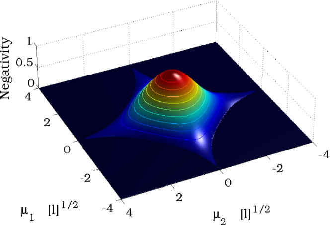
Figure 1: (Color online) The negativity as a function of the coupling strengths $\mu_{A}$ and $\mu_{B}$. ($\varsigma_{A}=\varsigma_{B}=1\,[\ell]^{1/2}$, $t=1\,[\ell]$, and $\theta=3\pi/5$) On the (dark blue) flat surface the negativity equals zero. The disentanglement time is finite unless $\mu_{A}$ or $\mu_{B}$ vanishes.

We now wish to examine the transition of the stochastic expectation of the density matrix from the initial maximally entangled singlet state to the mixture of the final outcomes, paying particular attention to the rate of the disentanglement. While for pure states, the entanglement is quantified by the von-Neumann entropy, there is no single measure of entanglement for mixed states. One of the standard measures is the negativity [18], $\frac{1}{2}(\left\|\rho^{T_{i}}\right\|-1)$, where $\rho^{T_{i}}$, the partial transpose with respect to $i$ of $\rho$, is obtained from $\rho$ by transposing the indices of system $i$, which is just minus the sum of the negative eigenvalues of the $\rho^{T_{i}}$ [19, 20].

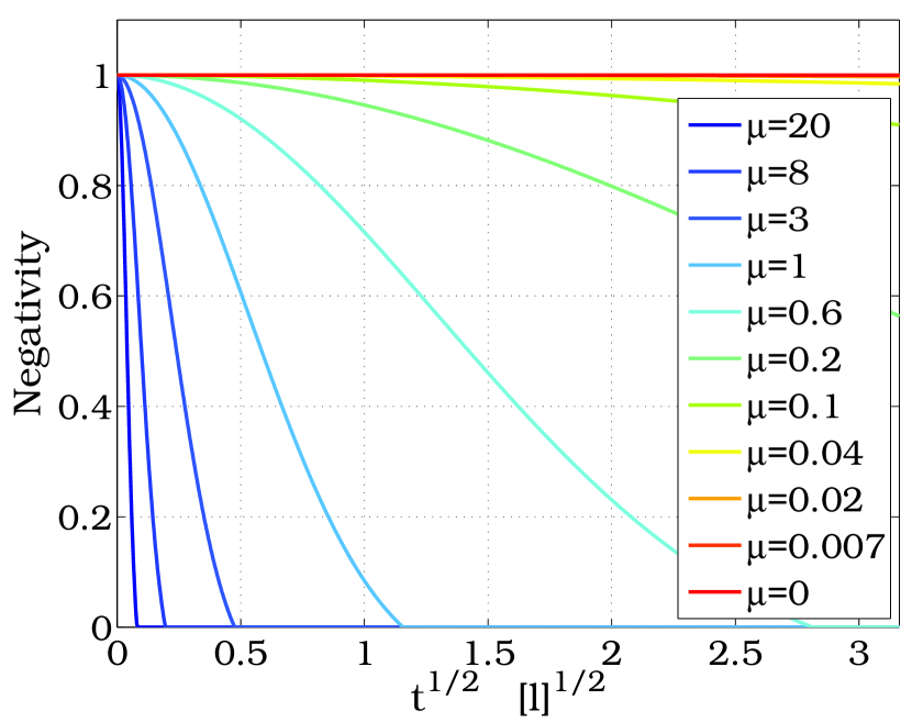
Figure 2: (Color online) The negativity as function of time for different values of the $\varsigma_{A}=\varsigma_{B}$. ($\theta=3\pi/5$, $\mu_{A}=\mu_{B}=1\,[\ell]^{-1}$) The legend gives the value of ${\varsigma_{i}}^{2}/8$ for each of the curves.

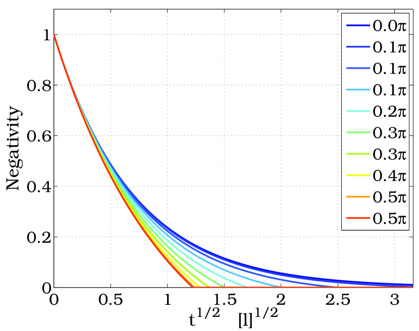
Figure 3: (Color online) The negativity as function of time and $\theta$. ($\varsigma_{A}=\varsigma_{B}=1\,[\ell]^{1/2}$, $\mu_{A}=\mu_{B}=1$) The legend gives the value of $\theta$ for each of the curves.

Numerical results are presented in figures (1-3). Figure (1) illustrates the dependence of the negativity on the coupling strengths, $\mu_{A}$ and $\mu_{B}$. We see that unless $\mu_{A}$ or $\mu_{B}$ vanishes, the disentanglement time is finite. This phenomenon, termed "entanglement sudden death" [21], is not unique to our setting and is typical of open systems dynamics [22]. For short times the rate of disentanglement is roughly dependent on $\sqrt{{\mu_{A}}^{2}+{\mu_{B}}^{2}}$, while for long times becomes linear. Figures (2) and (3) show the negativity as function of time for different values of $\varsigma_{A}=\varsigma_{B}$ and $\theta$, respectively.

5 Noise trajectories

Eq. (8) gives rise to an entropy conserving evolution. In particular, this means that a pure state remains pure. The trajectories realized by the $W_{i}(t)$ during the evolution fully specify the state’s history. However, as there is no means of determining these, all accessible information is contained in the state’s stochastic expectation. The trajectories can therefore be regarded as hidden-variables, i.e. indeterminable variables carrying information regarding the state of the system unavailable in the standard quantum mechanical description.

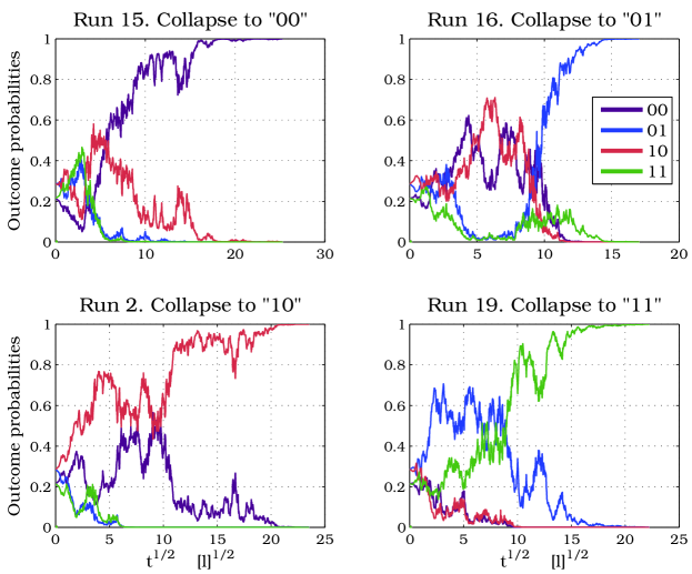
Figure 4: (Color online) Four realizations of the collapse process. The probabilities for the four different outcomes ($1\hat{=}\uparrow$, $0\hat{=}\downarrow$) are plotted as a function of time. $\mu_{A}=\mu_{B}=1\,[\ell]^{-1}$, $\varsigma_{A}=\varsigma_{B}=0.14\,[\ell]^{1/2}$ and $\theta=5\pi/{11}$. The same realization of $W_{A}(t)$ was used in all of the runs, whereas $W_{B}(t)$ varies from one run to the next. We see that the final outcome of particle $A$ depends on not only $W_{A}(t)$ but on $W_{B}(t)$ as well.

From the relation $dW_{i}(t)dW_{j}(t)=\delta_{ij}dt$ it does not follow that the trajectories are local hidden-variables. Indeed, any hidden-variable theory adhering to the statistical predictions of standard quantum mechanics must violate some Bell inequality, and as such our set up is manifestly nonlocal. Explicitly, this just means that the both $W_{A}(t)$ and $W_{B}(t)$ determine the final state of each of the particles (rather than $W_{i}(t)$ determining the final state of particle $i$ on its own). This point is illustrated in figures (4) and (5), which present the results of numerical iterative solutions to eq. (8) with randomly generated noise terms. Figure (4) explicitly shows how, for the same realization of $W_{A}(t)$, different realizations of $W_{B}(t)$ lead to different outcomes in the spin measurement of particle $A$ (and particle $B$). It is also interesting that in this case the probabilities for the measurement outcomes no longer agree with those of quantum mechanics, as is evident from figure (5).

To see how this comes about we must go back to eq. (8). Even though it describes a pair of uncoupled systems, it gives rise to a potentially disentangling (and entangling) evolution, because each of the ${H_{i}}(t)$ depends on the full state of the system (${H_{i}}(t)={tr_{j\neq i}}[\rho(t)\hat{H}_{i}]$), and therefore on ${W_{j\neq i}}(s\leq t)$. Note, however, that this nonlocality does not allow for superluminal signalling since the trajectories are "hidden".

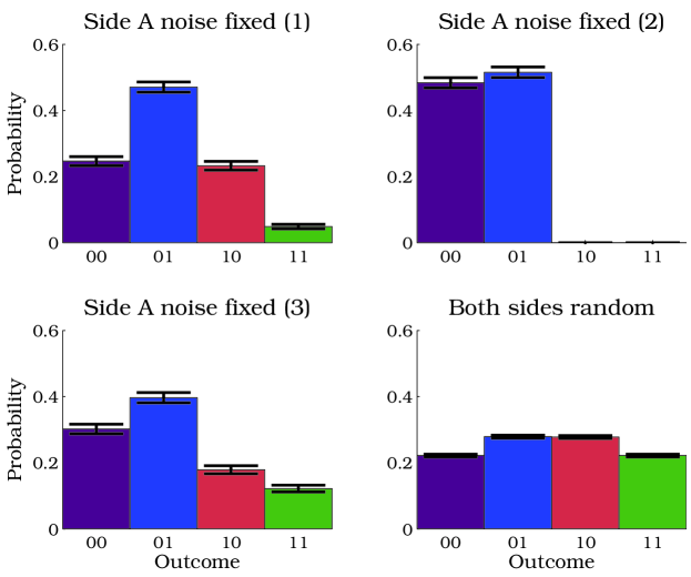
Figure 5: (Color online) Dependence of the outcome probabilities on the noise trajectories. The first three figures display the results of 1000 runs simulations, in which $W_{A}(t)$ is held fixed from run to the next, but realized differently in each simulation, while $W_{B}(t)$ varies from one run to the next. We see that different realizations of $W_{A}(t)$ lead to different outcome probabilities that do not agree with those of quantum mechanics. In the fourth figure, displaying the results of 10000 runs simulation, both $W_{A}(t)$ and $W_{B}(t)$ vary, and the quantum mechanical predictions are obtained.

6 Some concluding remarks

We have discussed Bohm’s formulation of the EPR experiment in the the energy-based stochastic reduction framework. In particular, we have seen how the presence of the measurement devices induces the reduction of the singlet state to the expected outcome product states with correct probabilities as predicted by the standard theory and have given the explicit time evolution of the process of disentanglement. As an extension of this idea, one may consider a problem with a natural degeneracy of some initial state where the presence of effective detectors of some type induces a perturbation in which stochastic reduction takes place, as in the asymptotic cluster decomposition of products of quantum fields reducing an $n$-body system to $m$ $k$-body systems, or the formation of local correlations in $n$-body systems such as liquids, or spontaneous symmetry breaking. In all these cases, due to the existence of continuous spectra, there will be some residual dispersion in the final state, although possibly very small. We are currently studying possible applications of the methods discussed here to such configurations.

References

References

- [1] Schrödinger E 1935 Naturwissenschaften 23 807
- [2] Gisin N 1984 Phys. Rev. Lett. 52 1657
- [3] Diósi L 1988 Phys. Lett. A 129 419
- [4] Gisin N 1989 Helv. Phys. Acta 62 363
- [5] Ghirardi G C, Pearle P and Rimini A 1990 Phys. Rev. A 42 78
- [6] Percival I 1994 Proc. Roy. Soc. Lond. A 447 189
- [7] Hughston L P 1996 Proc. Roy. Soc. Lond. A 452 953
- [8] Adler S L and Horwitz L P 2000 J. Math. Phys. 41 2485
- [9] Adler S L, Brody D C, Brun T A and Hughston L P 2001 J. Phys. A 34 8795
- [10] Bohm D 1951 Quantum Theory (New York: Prentice Hall)
- [11] Einstein A, Podolsky B and Rosen N 1935 Phys. Rev. 47 777
- [12] Bell J S 1964 Physics 1 195
- [13] Aspect A, Dalibard J and Roger G 1982 Phys. Rev. Lett. 49 1807
- [14] Brody D C and Hughston L P 2006 J. Phys. A 21 2885
- [15] Lüders G 1951 Ann. Phys. 8 322
- [16] Gorini V, Kossakowski A and Sudarshan E C G 1976 J. Math. Phys. 17 821
- [17] Lindblad G 1976 Commun. Math. Phys. 48 119
- [18] Vidal G and Werner R F 2002 Phys. Rev. A 65 032314
- [19] Peres A 1996 Phys. Rev. Lett. 77 1413
- [20] Horodecki M, Horodecki P and Horodecki R 1996 Phys. Lett. A 223 1
- [21] Yu T and Eberly J H 2006 Opt. Commun. 264 393
- [22] Dodd P J and Halliwell J J 2004 Phys. Rev. A 69 052105