Phenomenology of the 1/N_f Expansion for Field Theories in Extra Dimensions

Abstract

In this paper we review the properties of the 1/$N_{f}$ expansion in multidimensional theories. Contrary to the usual perturbative expansion it is renormalizable and contains only logarithmic divergencies. The price for it is the presence of ghost states which, however, in certain cases do not contribute to physical amplitudes. In this case the theory is unitary and one can calculate the cross-sections. As an example we consider the differential cross section of elastic $eq\rightarrow eq$ scattering in $D=7,11,...$-dimensional world. We look also for the unification of the gauge couplings in multidimensional Standard Model and its SUSY extension which takes place at energies lower than in 4 dimensions.

1 Introduction

Theories in extra dimensions are one of the best candidates for a new physics beyond the Standard Model Original ; review . The drawback of these theories is non-renormalizability since the coupling constant has negative dimension and perturbative expansion is seek of ultraviolet divergencies. Thus, one can deal with such theories as effective theories ratt valid up to some scale and consider them at the tree level in hope that some higher energy theory like a string theory will cure all the UV problems.

Recently we have shown that using the $1/N_{f}$ expansion KV the theory in multi-dimensional world is renormalizable and has only logarithmic divergencies contrary to the usual perturbative expansion. In this approach the propagators of the gauge fields acquire the improved UV behaviour $(p^{2})^{1-D/2}$ which has better convergence in loop integrals. This behaviour corresponds to conformal fixed points and leads to logarithmic divergences in any space time dimension greater than 4. For $D$ odd one has a non-integer power that manifests the idea of unparticle physics proposed recently by Georgi Georgi .

Effectively the $1/N_{f}$ expansion leads to the higher derivative theories which suffer from the presence of the ghost states widely discussed in the literature Nexpansion , unitarity . We argued in KV that in some cases these ghost states might be irrelevant since they do not contribute to the physical amplitudes. We present these arguments below. Provided this is true one can consider such amplitudes and calculate the cross-sections to compare them with the ones in 4 dimensional theories. We consider one of such examples.

Several years ago it was suggested that in extra dimensions the running of the couplings is power-like which leads to the early unification powerbehav . That was based on the Kaluza-Klein picture of extra dimensions and a special cut-off procedure of higher modes due to the non-renormalizability of the underlying theory. Contrary, in the case of the $1/N_{f}$ expansion in extra dimensions one has the renormalizable theory with logarithmic running, however, faster than in 4 dimensions. It leads to the approximate unification both in the Standard Model and in the MSSM.

2 The $1/N_{f}$ Expansion for Extra-Dimensional Theories

Here we briefly discuss the main features of the $1/N_{f}$ expansion in multidimensional space-time KV . As an example we consider the usual QED with $N_{f}$ fermion fields in $D$ dimensions, where $D$ takes an arbitrary odd value. The Lagrangian looks like

$${\cal L}=-\frac{1}{4}F_{\mu\nu}^{2}-\frac{1}{2\alpha}(\partial_{\mu}A_{\mu})^{2}+\bar{\psi_{i}}(i\hat{\partial}-m)\psi_{i}+\frac{e}{\sqrt{N_{f}}}\bar{\psi_{i}}\hat{A}\psi_{i},$$ (1)

where $F_{\mu\nu}\ =\ \partial_{\mu}A_{\nu}-\partial_{\nu}A_{\mu}$.

According to the general strategy of the $1/N_{f}$ expansion Nexpansion one first calculates the photon propagator in the leading order of $1/N_{f}$. Due to transversality of the polarization operator it is useful to apply the Landau gauge. Then in the leading order one has the following sequence of bubbles (see Fig.(1))

Figure 1: The chain of diagrams giving a contribution to the photon propagator in the zeroth order of the $1/N_{f}$ expansion

summed up into a geometrical progression. The resulting photon propagator takes the form

$$D_{\mu\nu}(p)=-\frac{i}{p^{2}}\left(g^{\mu\nu}-\frac{p^{\mu}p^{\nu}}{p^{2}}\right)\frac{1}{1+e^{2}f(D)(-p^{2})^{D/2-2}},$$ (2)

where

$$f(D)=\frac{\Gamma^{2}(D/2)\Gamma(2-D/2)}{2^{D-[D/2]-1}\Gamma(D)\pi^{D/2}}$$

and we put $m=0$ for simplicity.

It useful now to change the normalization of the gauge field $A_{\mu}\to A_{\mu}/e$ and introduce the dimensionless coupling $h$ associated with the triple vertex for the interaction of fermions with the gauge field KV . The new coupling $h$ is needed for the multiplicative renormalizability of the theory and provides the validity of the renormalization group pole equations Hooft . After this the effective Lagrangian takes the form

$${\cal L}_{eff} = -\frac{1}{4}F_{\mu\nu}\left(\frac{1}{e^{2}}+f(D)(\partial^{2})^{D/2-2}(1+h)\right)F_{\mu\nu}$$

$$-\frac{1}{2\alpha e^{2}}(\partial_{\mu}A_{\mu})^{2}+\bar{\psi_{i}}(i\hat{\partial}-m)\psi_{i}+\frac{\sqrt{h}}{\sqrt{N_{f}}}\bar{\psi_{i}}\hat{A}\psi_{i}.$$

In the non-Abelian case in addition one has the triple and quartic self-interaction of the gauge fields. These vertices, which are suppressed by $1/\sqrt{N_{f}}$ and $1/N_{f}$, respectively, obtain loop corrections of the same order in $1/N_{f}$. This leads to extra terms in effective Lagrangian. For more details see KV .

The Lagrangian (2) is written in multi-dimensional world. At high energies ($E>M_{c}$, where $M_{c}$ is the scale of extra dimensions) the higher-derivative term dominates, while at low energies ($E<M_{c}$) one has the usual Maxwell term, thus establishing the correspondence with the classical theory. To find connection to the four-dimensional world one has to assume some kind of compactification or localization. For example, within the brane-world scenario one may take the fermion fields localized on 4-dim brane and integrate over the extra dimensions. Then one gets the following relation between the D-dimensional and four dimensional couplings

$$e_{(D)}=e_{(4)}/V_{d},\ \ \ e_{(4)}\equiv\sqrt{h},$$

where $V_{d}\sim M_{c}^{d}$ is the volume of compact extra dimensions or localization volume. The new dimensionless coupling $h$ enters into the gauge transformation and plays the role of the gauge charge.

As follows from eq.(2) one has the modified Feynman rules with the photon propagator that decreases in the Euclidean region like $1/(p^{2})^{D/2-1}$, thus improving the UV behaviour in a theory. The only divergent graphs are those of the fermion propagator and the triple vertex. They are both logarithmically divergent for any odd D. The photon propagator is genuinely finite and may contain divergencies only in subgraphs. Therefore, due to the Ward identities in QED, one has vanishing beta-function and the coupling $h$ is not running. In the non-Abelian case this is not true and the beta-function is given by

$$\beta(h)=\frac{-\Gamma(D)(D-1)C_{A}\frac{\displaystyle h^{2}}{\displaystyle(1+h)^{2}}}{2^{[D/2]+2}\Gamma(2-D/2)\Gamma(D/2+1)\Gamma^{2}(D/2)N_{f}T}.$$ (4)

One can see that $\beta(h)>0$ for $D=5,9,...$, $\beta(h)<0$ for $D=7,11,...$ and then alternates with $D$. Hence, one has UV asymptotic freedom for dimensions $D=7,11,...$

Consider now the analytical properties of the propagator (2) and related problem of unitarity. Besides the cut starting from $4m^{2}$ it has poles in the complex $p^{2}$ plane. Hence, knowing the analytical structure, one can write down the Källen-Lehmann representation. It has two contributions: one comes from the pole structure and the other one is the continuous spectrum. Depending on a sign of $f(D)$ there are two possibilities: either one has a pole at the real axis and (possibly) pairs of complex conjugated poles ($f(D)<0$, D=5,9,…) or one has only pairs of complex conjugated poles ($f(D)>0$, D=7,11,…) and all the rest appears at the second Riemann sheet. In KV it was shown that the continuous spectrum has a positive spectral density and corresponds to the production of pairs of fermions. These states are present in the original spectrum and cause no problem with unitarity. One can show that all the cuts imposed on diagrams when applying Cutkosky rules in any order of perturbation theory lead to the usual asymptotic states on mass shell and no new states appear.

The problem comes with the poles. One can see that the pole terms come with negative sign and, therefore, correspond to the ghost states. For $D=5$ one has only one pole at the positive real semiaxis while for $D=7$ one has a pair of complex conjugated poles, as shown in Fig. 2.

Figure 2: The analytical structure of the gauge field propagator

The presence of those ghost states is the drawback of a theory. They signal of instability of the vacuum state. So one has either to try to get rid of the ghost poles or to make sure that they do not give a contribution to the physical amplitudes. It was shown in KV that the contribution of those states to the physical amplitudes is canceled in $D=7,11,...$ due to the complex conjugation of the poles in (2) and they do give contribution to the physical amplitudes in $D=5,9,...$

3 The Cross Section of Elastic Scattering

To find out the phenomenological consequences of extra-dimensional theories within our approach we calculate the cross section of elastic $e^{-}q$ scattering: $e^{-}q\rightarrow e^{-}q$. In the Standard Model for this process one has only one diagram in $t$-channel (see Fig.(3)) that gives the differential cross section Peskin

$$\frac{d\sigma_{SM}}{dt}\ =\ \frac{2\pi\alpha^{2}Q_{f}^{2}}{s^{2}}\left(\frac{s^{2}+u^{2}}{t^{2}}\right).$$ (5)

Figure 3: The $e^{-}q\rightarrow e^{-}q$ scattering process

To calculate the same cross section in multi-dimensional world we assume the brane world scenario local and consider the scattering of particles that are localized on 4-dim brane while the photon field propagates in the bulk and has the propagator given by (2). The interaction term on the brane now looks like

$$\frac{\sqrt{h}}{\sqrt{N_{f}}}\int d^{4}xd^{d}y\bar{\psi}(x)\gamma^{\mu}A_{\mu}^{a}(x,y)\psi(x)\delta^{d}(y).$$

Given this setup, to get the cross section one just has to replace the photon propagator in (5) by a modified one and to integrate over the extra dimensions:

$$\frac{1}{t}\ \Rightarrow\ \frac{(-)^{d/2}}{(2\pi)^{d}}\int\frac{d^{d}p}{(t-p^{2})\left(1/e^{2}_{(D)}+N_{f}f(D)(p^{2}-t)^{d/2}\right)}$$

To compare the cross section in multidimensional world with the one in the Standard Model we assume that the extra dimensions appear at some scale $M_{c}$: below this scale on has the usual 4-dim cross section and above this scale the full multi-dimensional theory is applied. So one has to merge the two cross sections at compactification scale $M_{c}$. Working in the center of mass frame and taking $\theta=\pi/2$ one gets $t=-s/2,u=-s/2$. Requiring that

$$\frac{d\sigma_{SM}}{dt}|_{s=M_{c}^{2}}\ =\ \frac{d\sigma_{D}}{dt}|_{s=M_{c}^{2}},$$ (6)

one gets the equation for $e^{2}_{(D)}$. Taking for example $D=7,11$ and $N_{f}=3$ we find numerically $1/e^{2}_{(7)}\simeq 0.2988M_{c}^{3},1/e^{2}_{(11)}\simeq 312.96M_{c}^{7}$. Finally we obtain the following expression for the differential cross section in $D=4+d$ dimensions in the c.m.f

$$\frac{d\sigma_{D}}{dt} =\frac{5\pi e^{2}Q_{f}^{2}}{2(2\pi)^{2d}}$$

$$\left(\int\frac{d^{d}p}{(s/2+p^{2})\left(XM_{c}^{d}+3f(D)(s/2+p^{2})^{d/2}\right)}\right)^{2},$$

where $X$ is found from (6) and it depends on the number of dimensions $D$.

As an illustration we show in Fig.4 the resulting cross section in the case of $D=7,11$ for $\theta=\pi/2$. The compactification scale $M_{c}$ is taken to be equal to 1 TeV. For comparison we also show the 4-dimensional cross section (5).

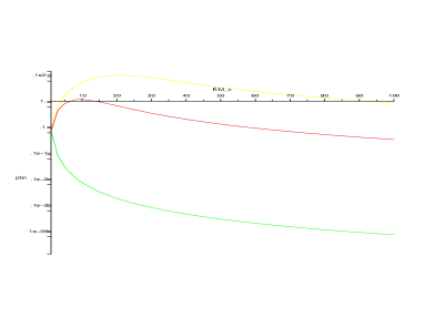
Figure 4: The differential cross section for $eq\rightarrow eq$ scattering

One can see, that above the compactification scale the cross sections differ essentially, however, asymptotically the exhibit the same behaviour decreasing like $1/s$ contrary to Kaluza-Klein approach and in agreement with the fixed point behaviour TMP .

4 The Gauge Coupling Unification

Here we would like to apply the $1/N_{f}$ expansion to the problem of the gauge coupling unification. As it is well known, the gauge coupling unification does not take place in the Standard Model but can be easily achieved in the MSSM. It occurs at very high energy scale of the order of $10^{16}$ GeV which is far beyond direct search. At the same time in powerbehav it was suggested that one can get early unification in theories in extra dimensions due to the power law running of the couplings.

Our approach to extra-dimensional theories based on the $1/N_{f}$ expansion allows us to look at this problem differently. We get the logariphmic running but with slightly different beta functions: for the $U(1)$ coupling constant we have the zero beta function that means that the $U(1)$ coupling does not run and for $SU(2)$ and $SU(3)$ couplings we have the beta function given by eq.(4). Substituting the proper Casimir operators and taking the number of families $N_{F}=3$ one can solve the RG equations numerically and check the unification.

We apply the following procedure: Below the unification scale we take the usual RG equations. Then we use the values of the couplings at the compactification scale as initial conditions for RG equations in extra dimensions and run the dimensionless couplings $\alpha_{i}=h_{i}/4\pi$ according to new equations. The scale of compactification is varied to get better unification.

The resulting curves for the inverse couplings in the case of the Standard Model are shown in Fig.5 for $D=7$. We would like to stress here that we do not have exact unification at one point but rather the triangle of the unification though much smaller than in the usual 4-dim SM. The compactification scale happens to be of the order of $M_{c}\sim 7\cdot 10^{12}$ GeV.

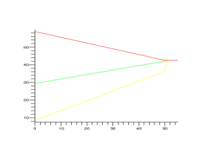
Figure 5: The running of the coupling constants in the SM

In the MSSM case one has to add the contributions of $N_{f}$ superpartners, however, the picture does not change much: qualitatively, unlike the 4-dim case, one has the same pattern. In Fig.6 for $D=7$ we show the plots for two possible choices of the compactification scale: on the left plot we take $M_{c}\sim 4\cdot 10^{10}$ GeV and on the right plot $M_{c}\sim 7\cdot 10^{12}$ GeV. In both the cases the SUSY scale is taken to be the same $M_{SuSy}\sim 500$ GeV.

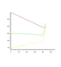
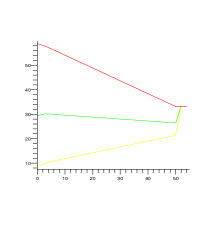
Figure 6: The running of the coupling constants in the MSSM

Again one can get approximate unification, the better the larger the compactification scale. From this point of view we do not see here much difference between the SM and the MSSM.

5 Conclusion

We conclude that within the $1/N_{f}$ approach the multi-dimensional theory can be made meaningful, renormalizable and manageable. And though it necessarily contains the ghost states in case when they are complex conjugated their contribution to physical amplitudes cancels and the theory seems to be unitary.

In such a theory one can calculate the cross sections of elementary processes assuming certain compactification (localization) scenario. These cross sections differ from those of the Standard Model in 4 dimensions but asymptotically have the naïve scaling behaviour and, hence, do not violate unitarity.

The running of dimensionless couplings in such theories remains logarithmic and allows one to get approximate unification of the gauge couplings both in the Standard Model and in the MSSM, though the unification scale happens to be rather high, yet lower than in the usual MSSM.

References

-
(1)
N.Arkani-Hamed, S.Dimopoulos, and G.R.Dvali, Phys.Lett. B429,
(1998) 263.
L.Randall and R.Sundrum, Phys.Rev.Let. 83, (1999) 3370; Phys.Rev.Let. 83, (1999) 4690. -
(2)
Yu.A.Kubyshin, hep-ph/0111027;
D.I.Kazakov, CERN-2006-003 [hep-ph/0411064]. - (3) R. Rattazzi, Cargese lectures on extra-dimensions (Springer, Cargese 2003), pp 461-517.
- (4) D.I.Kazakov and G.S.Vartanov, JHEP 06, (2007) 081; hep-th/0607177; hep-th/0702004.
-
(5)
H.Georgi, Phys.Rev.Lett. 98, (2007)
221601;
H.Georgi, Phys.Lett. B650, (2007) 275. -
(6)
I.Ya.Aref’eva, Theor.Math.Phys. 29, (1976) 147; Theor.Math.Phys. 31, (1977) 3.
E. Tomboulis, Phys.Lett. B70, (1977) 361; Phys.Lett. B97, (1980) 77; Phys.Rev.Lett. 52, (1984) 1173;
I.Antoniadis, E. Tomboulis, Phys.Rev.D 33, (1986) 2756. -
(7)
T.D.Lee and G.C.Wick, Nucl.Phys. B9, (1969) 209; Nucl.Phys. B10, (1969) 1.
S.Hawking, T.Hertog, Phys.Rev.D 65, (2002) 103515;
I.Antoniadis, E.Dudas, D.M.Ghilencea, Nucl.Phys. B767, (2007) 29. - (8) K.Dienes, E.Dudas, and T.Gherghetta, Phys.Lett. B436, (1998) 55; Nucl.Phys. B537, (1998) 47.
- (9) G.t’Hooft, Nucl. Phys. B61, (1973) 455.
- (10) M.Peskin and D.Schroeder, An Introduction to Quantum Field Theory (Westview Press, 1995) pp.555-563.
- (11) C.Csaki, C.Grojean, H.Murayama, L.Pilo and J.Terning, Phys.Rev.D 69, (2004) 055006.
- (12) D.I.Kazakov, G.S.Vartanov, Theor.Math.Phys., 147, (2006) 533.