MPP-2007-152
PSI-PR-07-06
UWThPh-2007-26
Electroweak and QCD corrections to Higgs production via
vector-boson fusion at the LHC
M. Ciccolini1, A. Denner1 and S. Dittmaier2,3
1 Paul Scherrer Institut, Würenlingen und Villigen,
CH-5232 Villigen PSI, Switzerland
2 Max-Planck-Institut für Physik
(Werner-Heisenberg-Institut),
D-80805 München, Germany
3 Faculty of Physics, University of Vienna,
A-1090 Vienna, Austria
Abstract:
The radiative corrections of the strong and electroweak interactions are calculated at next-to-leading order for Higgs-boson production in the weak-boson-fusion channel at hadron colliders. Specifically, the calculation includes all weak-boson fusion and quark–antiquark annihilation diagrams to Higgs-boson production in association with two hard jets, including all corresponding interferences. The results on the QCD corrections confirm that previously made approximations of neglecting -channel diagrams and interferences are well suited for predictions of Higgs production with dedicated vector-boson fusion cuts at the LHC. The electroweak corrections, which also include real corrections from incoming photons and leading heavy-Higgs-boson effects at two-loop order, are of the same size as the QCD corrections, viz. typically at the level of for a Higgs-boson mass up to . In general, both types of corrections do not simply rescale differential distributions, but induce distortions at the level of 10%. The discussed corrections have been implemented in a flexible Monte Carlo event generator.
October 2007
1 Introduction
The production of a Standard Model Higgs boson in association with two hard jets in the forward and backward regions of the detector—frequently quoted as the “vector-boson fusion” (VBF) channel—is a cornerstone in the Higgs search both in the ATLAS [1] and CMS [2] experiments at the LHC. This is not only true for the Higgs-mass range between 100 and , which is favoured by the global Standard Model fit to electroweak (EW) precision data [3], but also for a Higgs mass of the order of several up to the theoretical upper limit set by unitarity and triviality constraints. Higgs production in the VBF channel also plays an important role in the determination of Higgs couplings at the LHC (see e.g. Ref. [4]). Even bounds on non-standard couplings between Higgs and EW gauge bosons can be imposed from precision studies in this channel [5].
The production of Higgs+2jets receives two kinds of contributions at hadron colliders. The first type, where the Higgs boson couples to a weak boson that links two quark lines, is dominated by squared - and -channel-like diagrams and represents the genuine VBF channel. The hard jet pairs have a strong tendency to be forward–backward directed in contrast to other jet production mechanisms, offering a good background suppression (transverse-momentum and rapidity cuts on jets, jet rapidity gap, central-jet veto, etc.). Applying appropriate event selection criteria (see e.g. Refs. [6, 7, 8, 9, 10] and references in Refs. [11, 12]) it is possible to sufficiently suppress background and to enhance the VBF channel over the second Higgs+2jets production mechanism that mainly proceeds via strong interactions. In this second channel the Higgs boson is radiated off a heavy-quark loop that couples to any parton of the incoming hadrons via gluons [13, 14]. According to a recent estimate [15] hadronic production contributes about to the Higgs+2jets events for a Higgs mass of after applying VBF cuts. A next-to-leading order (NLO) analysis of this contribution [14] shows that its residual scale dependence is still of the order of 35%.
Higgs production in the VBF channel is a pure EW process in leading order (LO) involving only quark and antiquark parton distributions. As -channel diagrams and interferences tend to be suppressed, especially when imposing VBF cuts, the cross section can be approximated by the contribution of squared - and -channel diagrams only. The corresponding QCD corrections reduce to vertex corrections to the weak-boson–quark coupling. Explicit NLO QCD calculations in this approximation [11, 16, 17, 18, 19] confirm the expectation that these QCD corrections are small, because they are shifted to the parton distribution functions (PDFs) via QCD factorization to a large extent. The resulting QCD corrections are of the order of and reduce the remaining factorization and renormalization scale dependence of the NLO cross section to a few per cent.
In a recent letter [20] we completed the existing NLO calculations for the VBF channel in two respects. Firstly, we added the full NLO EW corrections. Secondly, we calculated the NLO QCD corrections including, for the first time, the complete set of QCD diagrams, namely the -, -, and -channel contributions, as well as all interferences. Focussing on the integrated cross section (with and without dedicated VBF selection cuts), we discussed the impact of EW and QCD corrections in the favoured Higgs-mass range between 100 and . We found that the previously unknown NLO EW corrections are of the order of and, thus, as important as the QCD corrections. In the EW corrections we also take into account real corrections induced by photons in the initial state and QED corrections implicitly contained in the DGLAP evolution of PDFs. We found that these photon-induced processes lead to corrections at the per-cent level.
In this paper we describe more details of our calculation, which is performed in a widely analogous way to the EW and QCD corrections to the Higgs decay fermions [21, 22]. We classify the NLO QCD corrections into four different categories; the previously known corrections [11, 16, 17, 18, 19] are contained in one of these categories. Moreover, we extend our numerical discussion of the EW and QCD corrections in two respects. We now consider cross sections for Higgs masses above , including the leading EW two-loop corrections for a heavy Higgs boson using the results of Ref. [23], and we discuss differential distributions in transverse momenta, in rapidities, in the azimuthal angle difference of the tagging jets, and in the jet–jet invariant mass. We pay particular attention to the issue of distortions in distributions induced by radiative corrections, because such distortions usually are the signature of non-standard couplings.
2 Details of the calculation
2.1 General setup
At LO, the hadronic production of Higgs+2jets via weak bosons receives contributions from the partonic processes , , , and . For each relevant configuration of external quark flavours one or two of the topologies shown in Figure 1 contribute.
All LO and one-loop NLO diagrams are related by crossing symmetry to the corresponding decay amplitude . The QCD and EW NLO corrections to these decays were discussed in detail in Refs. [21, 22], in particular a representative set of Feynman diagrams can be found there.
To be more specific, we first show how the lowest-order and loop amplitudes for subprocesses of the type can be obtained from the corresponding results for . The basic lowest-order decay amplitudes involving - or -boson exchange, called with , have been defined in Eq. (2.8) of Ref. [21]; the two potentially relevant tree diagrams are shown in Figure 3; the corresponding squares and interference are illustrated in Figure 3.
The external momenta , helicities , and colour indices are assigned to the scattering particles according to
| (2.1) |
In order to compactify notation, we omit the labels , , , etc. in the amplitudes of the scattering process, i.e. we implicitly have , and abbreviate the helicity and momentum assignment in as , etc.. Note that momenta and helicities crossed into the initial state receive a sign change. In this notation the lowest-order amplitudes for the six basic flavour channels in read
| (2.2) |
where are generation indices, are quark-mixing matrix elements, and is one of the two colour operators
| (2.3) |
which are relevant to span a general amplitude in colour space. The second operator , which involves the Gell-Mann matrices , becomes relevant in the QCD corrections discussed below. The relative sign between the two amplitude contributions on the r.h.s. of (2.2) originates from their different fermion-number flow. In Section 2 of Ref. [21] the calculation of is described in terms of Weyl–van-der-Waerden spinor products in the conventions of Ref. [24], where and are spinors corresponding to external momenta. We note that complex conjugate products (but not ) receive an additional sign factor for each crossed momentum involved in the product.
The lowest-order and loop amplitudes for subprocesses of the type and can be obtained as follows. We assign the external momenta, helicities, and colour indices as
| (2.4) |
Then the corresponding amplitudes can be obtained via crossing symmetry from those for the process (2.1) as
| (2.5) |
When calculating the corresponding cross sections, symmetry factors 1/2 must be taken into account for identical fermions or antifermions in the final state.
In our calculation we neglect external quark masses whenever possible, i.e. everywhere but in the mass-singular logarithms. In (2.2) we made the CKM matrix elements explicit. Note that only absolute values of the CKM matrix elements survive after squaring the amplitudes; for the squared W-mediated diagrams this is obvious, for the interference between W- and Z-mediated diagrams results after contraction of the CKM matrix elements with Kronecker deltas. Numerically, only the mixing among the first two generations could be relevant, but its impact on Higgs production via VBF was found to be negligible. Since the contributions of external b quarks are suppressed, either by bottom densities or by -channel suppression, we optionally include b quarks in the initial and final states in our LO predictions, but not in the calculation of corrections.
2.2 Evaluation of NLO corrections
Evaluating particle processes at the NLO level is non-trivial, both in the analytical and numerical parts of the calculation. In order to ensure the correctness of our results we have evaluated each ingredient twice, resulting in two completely independent computer codes yielding results in mutual agreement. The actual calculation of virtual and real NLO corrections for the partonic processes is performed along the same lines as described in Ref. [21, 22] for the decays . Therefore, we only repeat the salient features of the evaluation.
(i) Virtual corrections
The virtual corrections modify the partonic processes that are already present at LO; there are about 200 one-loop diagrams per tree diagram in each flavour channel. At NLO these corrections are induced by self-energy, vertex, box (4-point), and pentagon (5-point) diagrams. The calculation of the EW one-loop diagrams has been performed both in the conventional ’t Hooft–Feynman gauge and in the background-field formalism using the conventions of Refs. [25] and [26], respectively. The QCD one-loop diagrams are evaluated in ’t Hooft–Feynman gauge.
In contrast to the - and -channel contributions (first two diagrams in Figure 1), the -channel diagrams (last diagram in Figure 1) contain resonant W- or Z-boson propagators that require a proper inclusion of the finite gauge-boson widths. For the implementation of the finite widths we use the complex-mass scheme, which was introduced in Ref. [27] for lowest-order calculations and generalized to the one-loop level in Ref. [28]. In this approach the W- and Z-boson masses are consistently considered as complex quantities, defined as the locations of the propagator poles in the complex plane. This leads to complex couplings and, in particular, a complex weak mixing angle. The scheme fully respects all relations that follow from gauge invariance. A brief description of this scheme can also be found in Ref. [29].
The amplitudes have been generated with FeynArts, using the two independent versions 1 and 3, as described in Refs. [30] and [31], respectively. The algebraic evaluation has been performed in two completely independent ways. One calculation is based on an in-house program written in Mathematica, the other has been completed with the help of FormCalc [32]. The amplitudes are expressed in terms of standard matrix elements and coefficients, which contain the tensor integrals, as described in the appendix of Ref. [33].
The tensor integrals are evaluated as in the calculation of the corrections to [28, 34]. They are recursively reduced to master integrals at the numerical level. The scalar master integrals are evaluated for complex masses using the methods and results of Ref. [35]. UV divergences are regulated dimensionally and IR divergences with an infinitesimal photon or gluon mass. Tensor and scalar 5-point functions are directly expressed in terms of 4-point integrals [36, 37]. Tensor 4-point and 3-point integrals are reduced to scalar integrals with the Passarino–Veltman algorithm [38] as long as no small Gram determinant appears in the reduction. If small Gram determinants occur, we expand the tensor coefficients about the limit of vanishing Gram determinants and possibly other kinematical determinants, as described in Ref. [37] in detail.
Since corrections due to Higgs-boson self-interactions become important for large Higgs-boson masses, we have included the dominant two-loop corrections to the vertex proportional to in the large-Higgs-mass limit which were calculated in Ref. [23]. Specifically, we include this effect via a correction factor
| (2.6) |
to the squares of the basic LO amplitudes in the - and -channel. We do not include this correction in the (suppressed) -channel contributions, because the underlying assumption in the derivation of that is much larger than any other relevant scale is spoiled by the invariant that can be of the order of or larger. We do not apply to interferences either, because this would require a more complicated structure in the correction (involving more than one form factor). The impact of corrections on interferences and -channel contributions is certainly negligible, since these effects are suppressed themselves.
(ii) Real corrections
The matrix elements for the real corrections (photonic/gluonic bremsstrahlung and photon-/gluon-induced processes) are obtained via crossing from the bremsstrahlung corrections to the related Higgs decays, . Explicit amplitudes for are given in Section 4.1 of Ref. [21] in terms of spinor products; for such results can be found in Section 3.3 of Ref. [22]. The matrix elements relevant for the calculation presented here have been checked against results obtained with Madgraph [39].
The bremsstrahlung corrections involve singularities from soft or collinear photon/gluon emission; the photon-/gluon-induced processes contain singularities from collinear initial-state splittings. Soft singularities, which are regularized by an infinitesimal photon/gluon mass, cancel between virtual and bremsstrahlung corrections. Collinear singularities connected to the initial or final state are regularized by small quark masses, which appear only in logarithms. While singularities connected to collinear configurations in the final state cancel for “collinear-safe” observables automatically after applying a jet algorithm, singularities connected to collinear initial-state splittings are removed via factorization by PDF redefinitions, as described in more detail in Section 2.5.
Technically, the soft and collinear singularities for real photon emission are isolated both in the dipole subtraction method following Ref. [40] and in the phase-space slicing method. For photons in the initial state the subtraction and slicing variants described in Ref. [41] are applied. The results presented in the following are obtained with the subtraction method, which numerically performs better.
The phase-space integration is performed with Monte Carlo techniques. One of our two codes employs a multi-channel Monte Carlo generator [42] similar to the one implemented in RacoonWW [27, 43]. Our second code uses a different implementation of a multi-channel Monte Carlo generator with adaptive weight optimization.
2.3 Classification of QCD corrections
As QCD corrections to Higgs production via VBF we consider the interference of VBF diagrams of the type shown in Figure 1 with the virtual QCD corrections arising from gluon exchange, gluon fusion, and gluon splitting. We also take into account the contributions from real gluon emission and gluon-induced processes. We classify these corrections in the same way as done for the QCD corrections to described in Ref. [22] upon considering possible contributions to the squared amplitude. The amplitude itself receives contributions from one of the two generic tree diagrams shown in Figure 3 or from both. Thus, the square of this amplitude receives contributions from squared and interference diagrams of the types depicted in Figure 3. Type (A) corresponds to the squares of each of the Born diagrams, type (B) to their interference if two Born diagrams exist.
After this preliminary consideration we define four different categories of QCD corrections. Examples of interference diagrams belonging to these categories are shown in Figure 4, the corresponding virtual QCD correction diagrams are depicted in Figure 5.
-
(a)
“Diagonal” QCD corrections to squared tree diagrams comprise all interference diagrams resulting from diagram (A) of Figure 3 by adding one additional gluon. Cut diagrams in which the gluon does not cross the cut correspond to virtual one-loop corrections, the ones where the gluon crosses the cut correspond to real gluon radiation. Note that interference diagrams in which the gluon connects the two closed quark lines identically vanish, because their colour structure is proportional to , where is a Gell-Mann matrix. Thus, the only relevant one-loop diagrams in this category are gluonic corrections to the vertex, as illustrated in the first diagram of Figure 5; the real corrections are induced by the corresponding gluon bremsstrahlung diagrams.
\SetScale.9
Figure 4: Categories of interference diagrams contributing to the QCD corrections. Figure 5: Basic diagrams contributing to the virtual QCD corrections to where and . The categories of QCD corrections, (a)–(d), to which the diagrams contribute are indicated. Previous calculations [11, 16, 17, 18, 19] of NLO QCD corrections focused on this category of corrections to - and -channel contributions only. This approximation is motivated by the smallness of -channel contributions, at least in the kinematic domain relevant for Higgs production via VBF, and by the suppression of all types of interferences in lowest order. Both of these suppressions are due to strong enhancements in the - and -channel weak-boson propagators that receive a small momentum transfer; only in contributions to squared amplitudes that are related to squared - and -channel LO graphs four enhancement factors of this kind can accumulate. For instance, interferences between two different - and -channel tree diagrams involve four enhanced propagators, but they pairwise peak in different regions of phase space (forward or backward scattered quarks).
-
(b)
QCD corrections to interferences comprise all interference diagrams resulting from diagram (B) of Figure 3 by adding one additional gluon, analogously to the previous category. Relevant one-loop diagrams are, thus, vertex corrections or pentagon diagrams, as illustrated in the first two diagrams of Figure 5.
-
(c)
Corrections induced by one splitting result from loop diagrams exemplified by the third graph in Figure 5. The remaining graphs are obtained by shifting the gluon to different positions at the same quark line and by interchanging the role of the two quark lines. Thus, the diagrams comprise not only box diagrams but also vertex diagrams. They do not interfere with Born diagrams with the same fermion-number flow because of the colour structure, i.e. in they only contribute if two Born diagrams exist.
Some of the squared diagrams of this category actually correspond to (collinear-singular) real NLO QCD corrections to loop-induced jet production, e.g. or . Here we consider only the interference contributions of the loop diagrams of this category with the lowest-order diagrams where the Higgs boson couples to a weak boson (see Figure 1), resulting in a UV- and IR- (soft and collinear) finite correction.
-
(d)
Corrections induced by two splittings (gg fusion) result from diagrams exemplified by the fourth graph in Figure 5. There are precisely two graphs with opposite fermion-number flow in the loop. Again, owing to the colour structure (see also below), these diagrams do not interfere with Born diagrams with the same fermion-number flow, i.e. the existence of two Born diagrams is needed.
The squared diagrams of this category actually correspond to (collinear-singular) real NNLO QCD corrections to loop-induced Higgs production via gluon fusion, . The considered interference contributions of the loop diagrams of this category with the lowest-order diagrams of Figure 1, however, again yield a UV- and IR- (soft and collinear) finite correction.
This category of QCD corrections was recently considered in the approximation of an infinitely heavy top quark in Ref. [44] and found to be suppressed. There it was also argued that QCD corrections to these small contributions might be sizeable, because further gluon exchange between the two incoming (anti-)quarks enables an interference with the tree diagram with the same fermion-number flow, thereby receiving an enhancement by four propagators with small momentum transfer. This contribution has very recently been studied in Ref. [45] and found to be completely negligible owing to the appearance of several other suppression mechanisms.
2.4 Structure of virtual corrections
Since the colour flow in EW loop diagrams is the same as in the corresponding lowest-order diagrams, the EW one-loop amplitudes can be decomposed into colour- and CKM-stripped amplitudes exactly in the same way as done in lowest order, where we decomposed in terms of (2.2).
According to the above classification, the QCD one-loop amplitudes of category (a) as well as the vertex corrections of category (b) involve only the colour operator of (2.3), while the pentagon diagrams of category (b) and all loops of categories (c) and (d) involve only the colour operator . Thus, we can decompose the amplitudes , etc., into colour- and CKM-stripped parts , etc., as follows
| (2.7) | |||||
Note that W-mediated parts do not receive contributions of categories (c) and (d).
Since the lowest-order amplitudes only involve colour operators , the following colour sums appear in the calculation of squared lowest-order amplitudes and of interferences between one-loop and lowest-order matrix elements:
| (2.8) |
where stands for the sum over the colour indices , and is the colour factor for a quark. Squared Born diagrams, as illustrated in type (A) of Figure 3, are proportional to , lowest-order interference diagrams of type (B) are proportional to . The situation is analogous for all EW one-loop diagrams. By definition, category (a) of the gluonic diagrams comprises all one-loop QCD corrections proportional to . In category (b), the vertex corrections are proportional to and the pentagons to . Categories (c) and (d) receive only contributions from ; interferences of one-loop diagrams like (c) and (d) in Figure 5 with Born diagrams of the same fermion-number flow vanish because of . Finally, for the one-loop corrections to the squared matrix elements we obtain
| (2.9) | |||||||
As already observed for the squared LO amplitudes, also here only absolute values of the CKM matrix elements, such as , contribute after contracting the Kronecker deltas of the generation indices.
2.5 Hadronic cross section
The hadronic cross section for colliding protons results from the partonic cross section upon convolution with the parton densities , which corresponds to parton carrying the fraction of the proton momentum (),
| (2.10) |
where is the factorization scale that separates the hard partonic process from the soft physics contained in the PDFs. The sum over the partons includes all quarks, antiquarks, gluons, and the photon. In LO only quarks and/or antiquarks are present in the initial state, in NLO also processes with one gluon or photon contribute. In detail the NLO parton cross sections read
| (2.11) |
where generically stands for any relevant quark or antiquark. The LO and virtual one-loop contributions (“LO” and “virt”) involve the partonic kinematics, while real emission contributions (“real”) are of the type with one additional light (anti)quark, gluon, or photon in the final state. The calculation of these subcontributions has been briefly described in the previous sections. The contribution called “fact” results from the PDF redefinition necessary to absorb collinear initial-state singularities into the PDFs via factorization, so that the partonic cross sections are free of such singularities. This separation introduces a logarithmic dependence on the factorization scale in that compensates the implicit dependence in the PDFs in NLO accuracy. The factorization explicitly proceeds as follows.
The virtual and real contributions of the parton cross sections contain mass singularities of the form and , which are due to collinear gluon/photon radiation off the initial-state quarks or due to a collinear splitting of initial-state gluons or photons. For processes that in LO involve only quarks and/or antiquarks in the initial state, the factorization is achieved by replacing the (anti-)quark distribution according to (see e.g. Ref. [41])
| (2.12) | |||||||
where are the so-called coefficient functions, and the splitting functions are defined as
| (2.13) |
Starting from the hadronic LO cross section after the substitution (2.12), the factorization contributions correspond to the terms of and involving the PDF of and . The replacement (2.12) defines the same finite coefficient functions as the usual -dimensional regularization for exactly massless partons where the terms appear as poles. The actual form of the coefficient functions defines the finite parts of the NLO corrections and, thus, the factorization scheme. Following standard definitions of QCD, we distinguish the and DIS-like schemes which are formally defined by
| (2.14) |
The scheme is motivated by formal simplicity, because it merely rearranges the IR-divergent terms (plus some trivial constants) as defined in dimensional regularization. The DIS-like scheme is defined in such a way that the deep inelastic scattering (DIS) structure function does not receive any corrections; in other words, the radiative corrections to electron–proton DIS are implicitly contained in the PDFs.
Whatever scheme has been adopted in the extraction of PDFs from experimental data, the same scheme has to be used when predictions for other experiments are made using these PDFs. In particular, the absorption of the collinear singularities of both QCD and QED origin into PDFs requires the inclusion of the corresponding QCD and QED corrections into the Dokshitzer–Gribov–Lipatov–Altarelli–Parisi (DGLAP) evolution of these distributions and into their fit to experimental data. We use the MRST2004QED PDFs [46] which consistently include QCD and QED NLO corrections. These PDFs include a photon distribution function for the proton and thus allow to take into account photon-induced partonic processes. As explained in Ref. [41], the consistent use of these PDFs requires the factorization scheme for the QCD corrections, but the DIS scheme for the QED corrections, i.e. we employ and of (2.14) for the QCD, but and for the QED corrections.
3 Numerical results
3.1 Input parameters and setup
We use the following set of input parameters [47],
| (3.7) |
If not stated otherwise, the Higgs-boson mass is set to
| (3.8) |
Using the complex-mass scheme [34], we employ a fixed width in the resonant W- and Z-boson propagators in contrast to the approach used at LEP to fit the W and Z resonances, where running widths are taken. Therefore, we have to convert the “on-shell” values of and (), resulting from LEP, to the “pole values” denoted by and . The relation between the two sets of values is given by [48]
| (3.9) |
leading to
| (3.12) |
We make use of these mass parameters in the numerics discussed below, although the difference between using or would be hardly visible.
The masses of the light quarks are adjusted to reproduce the hadronic contribution to the photonic vacuum polarization of Ref. [49]. Since quark mixing effects are suppressed111We checked that the cross section without cuts changes by one per mille and the one with VBF cuts by less than 0.01% when using a realistic quark mixing matrix. we neglect quark mixing and use a unit CKM matrix.
We use the scheme, i.e. we derive the electromagnetic coupling constant from the Fermi constant according to
| (3.13) |
In this scheme, the weak corrections to muon decay are included in the charge renormalization constant (see e.g. Ref. [50]). As a consequence, the EW corrections are practically independent of the masses of the light quarks. Moreover, this definition effectively resums the contributions associated with the running of from zero to the W-boson mass and absorbs leading universal corrections from the parameter into the LO amplitude.
We use the MRST2004QED PDFs [46] which consistently include QED corrections. Since no associated LO PDFs exist, we use these distributions both for LO and NLO predictions. We do not include processes with external bottom quarks in our default set-up. These are suppressed either because of the smallness of the b-quark densities or due to -channel suppression. Partonic processes involving b quarks are, however, included in our code in LO. As discussed in Section 3.4, these contributions are at the level of a few per cent. In contrast to Ref. [20], we use (instead of ) as factorization scale both for QCD and QED collinear contributions, which is a better scale choice when considering large Higgs-boson masses. For the calculation of the strong coupling constant we employ as the default renormalization scale, include 5 flavours in the two-loop running, and fix .
Jet reconstruction from final-state partons is performed using the -algorithm [51] as described in Ref. [52]. Jets are reconstructed from partons of pseudorapidity using a jet resolution parameter . Real photons are recombined with jets according to the same algorithm. Thus, in real photon radiation events, final states may consist of jets plus a real identifiable photon, or of jets only.
We study total cross sections and cross sections for the set of experimental “VBF cuts” defined in Ref. [18]. These cuts are expected to significantly suppress backgrounds to VBF processes, enhancing the signal-to-background ratio. We require at least two hard jets with
| (3.14) |
where is the transverse momentum of the jet and its rapidity. Two tagging jets and are defined as the two jets passing the cuts (3.14) with highest such that . Furthermore, we require that the tagging jets have a large rapidity separation and reside in opposite detector hemispheres:
| (3.15) |
All presented results have been obtained using the subtraction method. For the results in the tables we used events for the setup with VBF cuts and events without cuts. For the plots of and factorization scale dependence we generated events without cuts and events with VBF cuts. The plots for the distributions are based on events. Generally, the real corrections and the finite virtual QCD corrections are only calculated for each 10th event, the finite virtual EW corrections only for each 100th event.
3.2 Results for integrated cross sections
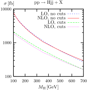
We first consider results for integrated cross sections. In Figure 6 we plot the total cross section with and without VBF cuts as a function of the Higgs-boson mass. In the left panel we show the absolute predictions in LO and in NLO including QCD and EW corrections. For to about the results without cuts are larger by a factor 2–4, while for this factor reduces to 1.7. In the right panel we show the relative QCD and EW corrections separately. For Higgs-boson masses in the range –, without cuts, the QCD corrections drop from +5% to 0%, and the EW corrections are about depending only weakly on the Higgs-boson mass. For very small Higgs-boson masses, QCD and EW corrections cancel each other substantially. With VBF cuts the EW corrections are somewhat more negative, while the QCD corrections vary between and . For higher Higgs-boson masses, the QCD corrections do not change much and reach and at without cuts and with VBF cuts, respectively. The EW corrections increase steadily with the Higgs-boson mass up to and at without cuts and with VBF cuts, respectively. In the EW corrections the WW, ZZ, and tt thresholds are clearly visible.

It is interesting to note that, at least for Higgs-boson masses below , the EW corrections to the full VBF channel are similar in size and sign to the subreactions [50]. Compared to the related decays [21, 22] the size is similar, but for low Higgs masses of the sign is different.
In Table 2 we present numbers for integrated cross sections for , 150, 200, 400, and without any cuts and in Table 2 results for the VBF cuts defined above.
120 150 200 400 700 5943(1) 4331(1) 2855.4(6) 900.7(1) 270.51(4) 5872(2) 4202(2) 2765(1) 871.8(3) 294.33(9)
120 150 200 400 700 1876.3(5) 1589.8(4) 1221.1(3) 487.31(9) 160.67(2) 1665(1) 1407.5(8) 1091.3(5) 435.4(2) 160.36(5)
We list the LO cross section , the cross section including NLO QCD and EW corrections, , and various contributions to the relative corrections. The complete EW corrections comprise the EW corrections resulting from loop diagrams and real photon radiation, , and the corrections from photon-induced processes . Furthermore, includes the dominant two-loop correction due to Higgs-boson self-interaction, which was introduced in Section 2.2. The QCD corrections are decomposed in the diagonal contributions , non-diagonal contributions , the contribution resulting from gluon splitting , and those from gluon-gluon fusion , as explained in Section 2.3.
The QCD corrections are dominated by the diagonal contributions, i.e. by the vector-boson–quark–antiquark vertex corrections to squared LO diagrams. All other contributions are at the per-mille level and even partially cancel each other. They are not enhanced by contributions of two - or -channel vector bosons with small virtuality and therefore even further suppressed when applying VBF cuts. The photon-induced EW corrections are about and reduce the EW corrections for small and intermediate . The two-loop correction is negligible in the low- region, but becomes important for large Higgs-boson masses. For this contribution yields and constitutes about of the total EW corrections. Obviously for Higgs masses in this region and above the perturbative expansion breaks down, and the two-loop factor might serve as an estimate of the theoretical uncertainty.
3.3 Subcontributions from channel and interference
Previous calculations of the VBF process [11, 16, 17, 18, 19] have consistently neglected -channel contributions (“Higgs strahlung”), which involve diagrams where one of the vector bosons can become resonant, as well as the interference between - and -channel fusion diagrams. To better understand the effect of these approximations we have calculated these contributions to the integrated cross section. In Table 4 and Table 4 we present, with and without VBF cuts, respectively, contributions from -channel processes, , and from /-channel interference terms , at both LO and NLO.
120 150 200 400 700 1294.4(2) 639.4(1) 244.26(4) 19.69 2.11 1582.1(4) 769.4(2) 289.80(9) 21.72(1) 2.29(1)
120 150 200 400 700
The NLO result does not include the corrections due to photon-induced processes, which cannot be split into the above subcontributions respecting gauge invariance.
While -interference terms, with or without VBF cuts, contribute less than to the cross section, -channel contributions are clearly non-negligible when no cuts are used. At LO (NLO), for they contribute () to the total cross section, while for this contribution decreases to (). For -channel processes contribute less than to the cross section, with and without VBF cuts. Thus, for increasing Higgs-boson masses, the contribution from Higgs-strahlung processes becomes less and less important compared to the contribution from pure fusion processes. When VBF cuts are used, both the -channel and -channel-interference contributions are strongly suppressed, yielding less than of the cross section for all the studied Higgs-boson masses. The comparably large NLO -channel contribution after VBF cuts originates from real gluon corrections with up to three jets in the final state, because in contrast to LO the two jets from the weak-boson decay, which tend to be aligned owing to a boost, are not forced to be the two well-separated tagging jets. We conclude that, applying typical experimental VBF cuts, the contributions from -channel diagrams and -channel interferences can be safely neglected.
3.4 Leading-order b-quark contributions
In this section we present the contributions arising at LO from processes that include b-quarks in the initial and/or final states. There are three types of contributions involving b quarks. The first type consists of -channel diagrams with a pair in the initial state, the second type comprises -channel diagrams with a pair in the final state, and the third type involves -channel diagrams with a pair in both the initial and the final state as well as all - and -channel diagrams where a b or quark goes from the initial state to the final state. In Table 6 we show, for different values, LO cross-section results without b-quark contributions, , the results including only initial-state b quarks, , the results including only final-state b quarks, , and including both initial- and final-state b quarks, .
120 150 200 400 700 5943(1) 4331(1) 2855.2(6) 900.7(1) 270.60(4) 5951(1) 4334(1) 2856.3(6) 900.7(1) 270.60(4) 0.13(2) 0.07(2) 0.04(2) 0.01(2) 0.00(2) 6054(1) 4386(1) 2876.7(6) 902.4(1) 270.77(4) 1.87(2) 1.27(2) 0.75(2) 0.19(2) 0.06(2) 6203(1) 4495(1) 2945.7(6) 919.5(2) 274.49(4) 4.37(2) 3.79(2) 3.17(2) 2.09(2) 1.44(2)
120 150 200 400 700 1876.1(5) 1589.8(4) 1221.1(3) 487.32(9) 160.66(2) 1876.1(5) 1589.8(4) 1221.1(3) 487.32(9) 160.66(2) 0.00(3) 0.00(2) 0.00(2) 0.00(2) 0.00(1) 1876.1(5) 1589.8(4) 1221.1(3) 487.32(9) 160.66(2) 0.00(3) 0.00(2) 0.00(2) 0.00(2) 0.00(1) 1918.5(5) 1624.5(4) 1246.3(3) 495.55(9) 162.75(2) 2.26(3) 2.18(2) 2.06(2) 1.69(2) 1.30(1)
The relative contributions arising from these subprocesses, , , and , are also shown. In Table 6 we present LO results including VBF cuts.
For low Higgs-boson masses and no cuts, final-state b quarks increase the LO cross section by up to . The increase due to initial-state b quarks is one per mille or less, being strongly suppressed due to the two bottom densities involved (-annihilation processes). Including both initial and final-state b quarks increases the total cross section by up to , a contribution that is similar in absolute value to the total EW correction, but opposite in sign. The contributions from final-state and/or initial-state b quarks decrease with increasing Higgs-boson mass. For , b-quark contributions from either final state or initial state become negligible, while simultaneous initial- and final-state b-quark corrections decrease to . When VBF cuts are imposed, b-quark contributions become less important. This is particularly noticeable in contributions arising from processes with final-state but no initial-state b quarks and vice versa, Higgs-strahlung processes of the form and . These are -channel processes and, as already shown in Section 3.3, this type of contributions are strongly suppressed by the VBF cuts.
3.5 Scale dependence
In Figures 8 and 8 we show the dependence of the total cross section on the factorization and renormalization scale for and , respectively.
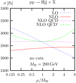
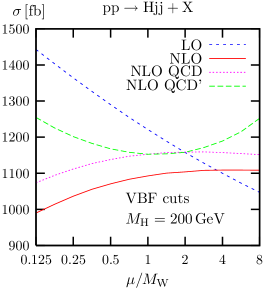


We relate the factorization scale , which applies to both QCD and QED contributions, and the renormalization scale to the W-boson mass as
| (3.16) |
and vary and between and . We study the scale dependence of the LO cross section, of the QCD-corrected NLO cross section, and of the complete NLO cross section including both QCD and EW corrections for . In addition we depict the QCD-corrected NLO cross section for the setup where (NLO QCD’). For , varying the scale up and down by a factor of 2 (8) changes the cross section by () in LO and by () in NLO for the set-up without cuts. With VBF cuts, the scale uncertainty amounts to () in LO and () in NLO. For , the scale uncertainty is reduced from () in LO to () in NLO for the cross section without cuts, and from () in LO to () in NLO for the cross section with VBF cuts. For , it is clearly seen from the results that is a more appropriate scale choice than . For this reason we have chosen as default scale in this paper, while we used in Ref. [20], where we only considered Higgs-boson masses comparable to .
3.6 Slicing cut dependence
In the slicing approach (as e.g. reviewed in Ref. [53]), phase-space regions where real photon/gluon emission and photon/gluon-induced processes contain soft or collinear singularities are defined by the auxiliary cutoff parameters In real photon/gluon radiation processes, the region
| (3.17) |
where is the photon/gluon momentum, the partonic centre-of-mass energy, and an infinitesimal photon/gluon mass, is treated in soft approximation. The regions determined by
| (3.18) |
where is the angle between any quark and the photon or gluon, are evaluated using collinear factorization. In photon- or gluon-induced processes, singularities arise only in the collinear region, i.e. a slicing cut on the angle between any final-state quark and the initial-state photon or gluon is sufficient to exclude the singularity from phase space. Specifically, we define this angular cut as in (3.18). The collinear-splitting singularities are also treated using collinear factorization.
In the remaining phase space no regulators (photon/gluon and quark masses) are used. Therefore, the slicing result is correct up to terms of and . In Figure 9 we show the dependence of the complete corrections to the cross section with VBF cuts on for fixed and the dependence on for fixed . The error bars reflect the uncertainty of the Monte Carlo integration.
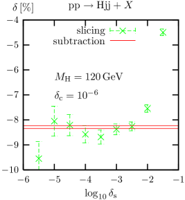

These results were obtained with events for the slicing method and events for the subtraction method, using as factorization and renormalization scale. For decreasing auxiliary parameters and , the slicing result reaches a plateau and becomes compatible with the subtraction result. The integration error in the result obtained with the slicing method increases for lower cut-off parameters. On the other hand, the subtraction results, for the same number of events, always show smaller integration errors.
3.7 Differential cross sections
In this section we consider results for distributions involving Higgs-boson and tagging-jet observables. We show results for in the setup including VBF cuts. For each distribution we plot the absolute predictions in LO and in NLO including QCD and EW corrections. In addition, we show the relative corrections, both the QCD and EW corrections separately, as well as their sum.
We first consider Higgs-boson observables and show the distribution in the transverse momentum in Figure 11. The differential cross section drops strongly with increasing , while both the relative EW and QCD corrections increase in size and reach for . It is interesting to note the differences between this result and the same distribution in Higgs-boson production via gluon-fusion, as e.g. shown in Ref. [54]. In weak-boson fusion, this distribution is broader and peaks at a much larger value of .


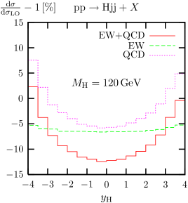
The distribution in the rapidity of the Higgs boson is presented in Figure 11. While the relative EW corrections depend only weakly on this variable, the QCD corrections show an increase for large rapidities. Total corrections decrease the differential cross section by more than in the central region, inducing an important change in the shape of this distribution.
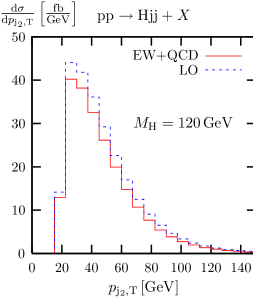
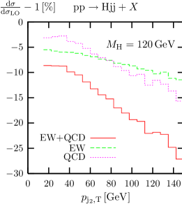
Figures 13 and 13 show the differential cross section as function of the transverse momentum of the harder and softer tagging jet, respectively. These distributions peak near or below and then drop strongly with increasing jet transverse momentum. QCD and EW corrections become more and more negative with increasing . For low transverse momentum these corrections are at the level of 5%, while for and they add up to about and for the harder and softer tagging jet, respectively. This induces a substantial change in shape of these distributions.


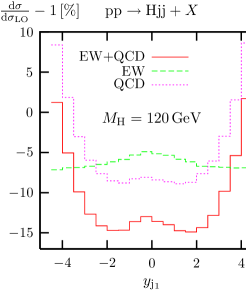
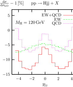
In Figures 15 and 15, we depict the distributions in the rapidities of the harder and softer tagging jet, respectively. It can be clearly seen that the tagging jets are forward and backward located. The EW corrections vary between and . The QCD corrections exhibit a strong dependence on the jet rapidities. For the harder tagging jet they are about in the central region but become positive for large rapidities, where they tend to compensate the EW corrections. For the softer tagging jet the variation for large rapidities is smaller, and the QCD corrections become small also near . Shape changes due to the full corrections can reach .


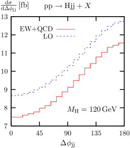
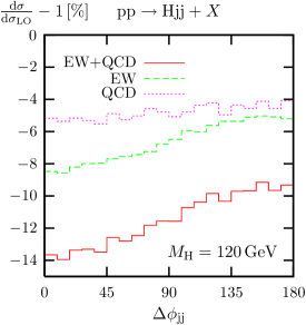
In Figure 17 we present the distribution in the azimuthal angle separation of the two tagging jets. This distribution is particularly sensitive to non-standard contributions to the vertices [18]. As expected for VBF processes, there is a large azimuthal angle separation between the two tagging jets. While QCD corrections are almost flat in this variable, the QCD+EW corrections exhibit a dependence on on the level of 4%.
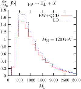

Finally, in Figure 17 we show the distribution in the tagging-jet-pair invariant mass . Tagging jets identified in EW processes have typically larger jet-pair invariant masses than the ones identified in QCD processes. Consequently, can be used to further suppress QCD backgrounds, as e.g. pointed out in Ref. [1]. This distribution peaks at approximately and is strongly suppressed for higher invariant-mass values. The EW corrections decrease with increasing and compensate the increasing QCD corrections for large invariant masses. The total correction is of the order of .
3.8 Comparison with related NLO QCD calculations
In this section we compare our results to those obtained with the software packages VV2H by M. Spira [55] and VBFNLO by D. Zeppenfeld et al.[56]222For this comparison we have employed the VV2H version dated July 23 2007, and VBFNLO-v.1.0.. These programs allow to calculate the LO and NLO-QCD-corrected cross sections for Higgs-boson production via VBF at hadron colliders. It is important to note that -channel contributions and -channel-interference contributions are not taken into account in these calculations. In particular, only the corrections that correspond to our class (a) of QCD contributions (see Section 2.3) are included. In order to allow for a tuned comparison, we here use only four quark flavours for the external partons, i.e. we have switched off the effect of initial- and final-state b quarks in the calculations. We compare the results of VV2H and VBFNLO with LO and NLO-QCD-corrected results of our code with -channel contributions and -channel-interference contributions switched off, . In addition, we give the results of our code, , with these contributions and all interferences switched on and including all EW corrections apart from photon-induced processes. We use CTEQ6 parton distributions [57] and our default set of input parameters.
We first compare our results to those obtained with VV2H, which implements the formulae presented in Ref. [16]. As it is not possible to include phase-space cuts in VV2H, we have only compared total cross sections. The results of this comparison can be found in Table 7. We observe that the LO cross sections agree within and the NLO corrected results within , a difference which is of the order of the statistical error.
120 150 170 200 400 700 4226.3(6) 3357.8(5) 2910.7(4) 2381.6(3) 817.6(1) 257.49(4) 4226.2(4) 3357.3(3) 2910.2(3) 2380.4(2) 817.33(8) 257.40(3) 5404.8(9) 3933.7(6) 3290.4(5) 2597.9(4) 834.5(1) 259.26(4) 4424(4) 3520(3) 3052(3) 2505(2) 858.4(7) 268.2(2) 4415(1) 3519.7(8) 3055.8(7) 2503.4(6) 858.8(2) 268.03(6) 5694(4) 4063(3) 3400(3) 2666(2) 839.0(7) 285.9(3)
Our complete predictions differ from the results of VV2H by up to 30% for low Higgs-boson masses and by a few per cent for high Higgs-boson masses. The bulk of this big difference for small values is due to the missing -channel contributions in VV2H.
We now turn to VBFNLO, which implements the results of Ref. [17]. As explained there, VBFNLO generates an isotropic Higgs-boson decay into two massless “leptons” (which represent or or final states), and imposes a cut on the invariant mass of the Higgs boson. In order to be able to compare with this setup, we have implemented a convolution with a Breit-Wigner distribution for the Higgs-boson in one of our codes. When performing this convolution we can either evaluate the matrix element for Higgs production for an on-shell Higgs boson or for a Higgs boson with an invariant mass given by the Breit-Wigner distribution. While the first variant is gauge invariant and corresponds to a pole approximation, the second one, which is implemented in VBFNLO, violates EW gauge invariance. Because of the simple structure of the matrix element, this might not be a problem in LO and if only QCD corrections are included. Both variants neglect contributions that do not involve a resonant Higgs boson, which is a good approximation for small Higgs-boson masses, where the Higgs-boson width is small, but not for large Higgs-boson masses, where the width is large. Using these two variants of our code, we have compared cross sections without imposing any cuts on the decay products of the Higgs boson and using a unit branching ratio. To define the integration region in the neighbourhood of the Higgs resonance, we employ the value for the Higgs-boson width calculated by VBFNLO.
The results for the cross section without cuts are compared in Table 9, while results including VBF cuts can be found in Table 9. The relative difference between the results of VBFNLO and the variant of our code with off-shell matrix elements, , is below for the total LO cross section and below for the NLO-QCD-corrected cross section, both with and without VBF cuts. This difference is of the order of the statistical error. The difference between and the variant with on-shell matrix elements, , is at the per-mille level for Higgs-boson masses below but strongly increases for a heavy Higgs boson. For and the differences reach about and , respectively, which illustrates the order of uncertainty without a more sophisticated treatment of off-shell effects of the Higgs boson including its decay. The results for are obtained with on-shell matrix elements only, since the off-shell matrix elements with EW corrections become gauge dependent. For small Higgs-boson masses and VBF cuts applied these predictions differ from those of VBFNLO by one per mille or less in LO and by 6–8%, the size of the EW corrections, in NLO. On the other hand, without cuts the big difference between and the other predictions at small values is again due to -channel contributions.
120 150 170 200 400 700 4216.8(6) 3350.0(5) 2904.5(4) 2377.9(3) 824.8(1) 284.28(8) 4218.4(2) 3351.1(2) 2905.2(1) 2378.8(1) 825.06(5) 284.35(2) 4216.8(6) 3349.7(5) 2903.6(4) 2373.5(3) 786.1(1) 206.15(3) 5394.0(9) 3925.1(6) 3282.5(5) 2590.5(4) 802.6(1) 207.75(3) 4407(3) 3512(3) 3050(2) 2500(2) 865.5(6) 296.8(3) 4405.3(3) 3512.0(2) 3049.5(2) 2500.5(2) 866.32(7) 296.63(3) 4409(3) 3511(3) 3043(4) 2494(2) 825.8(5) 214.7(1) 5678(5) 4055(3) 3392(3) 2659(2) 808.1(5) 229.0(2)
120 150 170 200 400 700 1683.2(3) 1430.6(2) 1287.3(2) 1104.6(1) 448.40(6) 159.44(3) 1683.32(5) 1430.75(4) 1287.74(4) 1104.76(3) 448.41(1) 159.431(5) 1682.6(3) 1430.4(2) 1287.5(2) 1103.6(1) 434.00(5) 123.13(1) 1682.9(3) 1429.6(2) 1287.0(2) 1103.2(1) 433.89(5) 123.11(1) 1726(1) 1459(2) 1307(1) 1118(1) 442.4(3) 155.0(2) 1725.3(2) 1458.9(1) 1308.8(1) 1117.6(1) 442.68(3) 154.71(1) 1724(2) 1460(1) 1310(2) 1118(1) 427.7(3) 118.0(1) 1595(2) 1351(2) 1228(1) 1045(1) 403.2(3) 124.82(9)
4 Conclusions
Higgs-boson production via weak-boson fusion is one of the most important processes in the search for and the study of a Standard Model-like Higgs boson at the LHC. In this paper we present the first calculation of the NLO electroweak corrections for this process and we extend previously existing approximate NLO QCD calculations by including -channel topologies (Higgs-strahlung processes) and all interferences, both in LO and NLO.
We find that the electroweak corrections are of the order of –, i.e. as large as the NLO QCD corrections. Real corrections induced by photons in the initial state increase LO results by roughly . More precisely, the electroweak corrections are approximately for Higgs masses below and for larger values steadily increase up to about for . For this Higgs-boson mass the leading two-loop effects in the heavy-Higgs limit, which are included in our calculation, become as large as the one-loop corrections. This signals the breakdown of perturbation theory for large Higgs-boson masses. We suggest that the theoretical uncertainty from missing higher-order corrections can be estimated by the size of the leading two-loop heavy-Higgs effects in this domain. Moreover, for owing to the large Higgs-boson width the on-shell approximation is not sufficient any more and a more sophisticated treatment including off-shell effects of the Higgs boson and its decay width is required.
We have implemented our calculation in a flexible Monte Carlo event generator, and studied differential distribution in Higgs-boson and tagging-jet observables. Specifically, we have presented results for distributions in transverse momenta, in rapidities, in the azimuthal angle difference of the tagging jets, and in the tagging-jet pair invariant mass. We found that QCD and electroweak corrections do not simply rescale differential distributions, but induce distortions at the level of .
Finally, we have compared our NLO QCD-corrected results with existing calculations, which only take into account -channel squared-diagram contributions. Working in this approximation, which renders the QCD corrections particularly simple, we found technical agreement between our results and the existing calculations within statistical integration errors. We also found that, when typical VBF cuts are applied, our full NLO QCD results agree with the ones in the -channel approximation within fractions of a per cent.
With the complete knowledge of NLO QCD and electroweak corrections, the theoretical uncertainty from missing higher-order effects should be of the order of 1–2% in total cross-section predictions for Higgs-boson masses in the range 100–. For distributions, the uncertainty will be larger in suppressed phase-space regions. The phenomenological error of the parton distributions contributes a further to the uncertainty, as reported in Ref. [17]. We thus conclude that the presented state-of-the-art results match the required precision for predictions at the LHC.
Acknowledgements
We thank M. Spira and D. Zeppenfeld for useful discussions. This work is supported in part by the European Community’s Marie-Curie Research Training Network under contract MRTN-CT-2006-035505 “Tools and Precision Calculations for Physics Discoveries at Colliders”. Finally, we thank the Galileo Galilei Institute for Theoretical Physics in Florence for the hospitality and the INFN for partial support during the completion of this work.
References
- [1] S. Asai et al., Eur. Phys. J. C 32S2 (2004) 19 [hep-ph/0402254].
- [2] S. Abdullin et al., Eur. Phys. J. C 39S2 (2005) 41.
- [3] J. Alcaraz et al. [LEPEWWG and LEP collaborations], LEPEWWG/2006-01, hep-ex/0612034.
- [4] M. Dührssen, S. Heinemeyer, H. Logan, D. Rainwater, G. Weiglein and D. Zeppenfeld, Phys. Rev. D 70 (2004) 113009 [hep-ph/0406323].
- [5] V. Hankele, G. Klämke, D. Zeppenfeld and T. Figy, Phys. Rev. D 74 (2006) 095001 [hep-ph/0609075].
- [6] V. D. Barger, R. J. N. Phillips and D. Zeppenfeld, Phys. Lett. B 346 (1995) 106 [hep-ph/9412276].
- [7] D. L. Rainwater and D. Zeppenfeld, JHEP 9712 (1997) 005 [hep-ph/9712271].
- [8] D. L. Rainwater, D. Zeppenfeld and K. Hagiwara, Phys. Rev. D 59 (1999) 014037 [hep-ph/9808468].
- [9] D. L. Rainwater and D. Zeppenfeld, Phys. Rev. D 60 (1999) 113004 [Erratum-ibid. D 61 (2000) 099901] [hep-ph/9906218].
- [10] V. Del Duca et al., JHEP 0610 (2006) 016 [hep-ph/0608158].
- [11] M. Spira, Fortsch. Phys. 46 (1998) 203 [hep-ph/9705337].
- [12] A. Djouadi, hep-ph/0503172.
- [13] V. Del Duca, W. Kilgore, C. Oleari, C. Schmidt and D. Zeppenfeld, Nucl. Phys. B 616 (2001) 367 [hep-ph/0108030].
- [14] J. M. Campbell, R. K. Ellis and G. Zanderighi, JHEP 0610 (2006) 028 [hep-ph/0608194].
- [15] A. Nikitenko and M. Vazquez Acosta, arXiv:0705.3585 [hep-ph].
- [16] T. Han, G. Valencia and S. Willenbrock, Phys. Rev. Lett. 69 (1992) 3274 [hep-ph/9206246].
- [17] T. Figy, C. Oleari and D. Zeppenfeld, Phys. Rev. D 68 (2003) 073005 [hep-ph/0306109].
- [18] T. Figy and D. Zeppenfeld, Phys. Lett. B 591 (2004) 297 [hep-ph/0403297].
- [19] E. L. Berger and J. Campbell, Phys. Rev. D 70 (2004) 073011 [hep-ph/0403194].
- [20] M. Ciccolini, A. Denner and S. Dittmaier, Phys. Rev. Lett. 99 (2007) 161803 [arXiv:0707.0381 [hep-ph]].
- [21] A. Bredenstein, A. Denner, S. Dittmaier and M. M. Weber, Phys. Rev. D 74 (2006) 013004 [hep-ph/0604011].
- [22] A. Bredenstein, A. Denner, S. Dittmaier and M. M. Weber, JHEP 0702 (2007) 080 [hep-ph/0611234].
-
[23]
A. Ghinculov,
Nucl. Phys. B 455 (1995) 21
[hep-ph/9507240];
A. Frink, B.A. Kniehl, D. Kreimer and K. Riesselmann, Phys. Rev. D 54 (1996) 4548 [hep-ph/9606310]. - [24] S. Dittmaier, Phys. Rev. D 59 (1999) 016007 [hep-ph/9805445].
- [25] A. Denner, Fortsch. Phys. 41 (1993) 307 [arXiv:0709.1075 [hep-ph]].
- [26] A. Denner, S. Dittmaier and G. Weiglein, Nucl. Phys. B 440 (1995) 95 [hep-ph/9410338].
- [27] A. Denner, S. Dittmaier, M. Roth and D. Wackeroth, Nucl. Phys. B 560 (1999) 33 [hep-ph/9904472].
- [28] A. Denner, S. Dittmaier, M. Roth and L. H. Wieders, Nucl. Phys. B 724 (2005) 247 [hep-ph/0505042].
- [29] A. Denner and S. Dittmaier, Nucl. Phys. Proc. Suppl. 160 (2006) 22 [hep-ph/0605312].
- [30] J. Küblbeck, M. Böhm and A. Denner, Comput. Phys. Commun. 60 (1990) 165; H. Eck and J. Küblbeck, Guide to FeynArts 1.0, University of Würzburg, 1992.
- [31] T. Hahn, Comput. Phys. Commun. 140 (2001) 418 [hep-ph/0012260].
-
[32]
T. Hahn and M. Pérez-Victoria,
Comput. Phys. Commun. 118 (1999) 153
[hep-ph/9807565];
T. Hahn, Nucl. Phys. Proc. Suppl. 89 (2000) 231 [hep-ph/0005029]. - [33] A. Denner, S. Dittmaier, M. Roth and M.M. Weber, Nucl. Phys. B 660 (2003) 289 [hep-ph/0302198].
- [34] A. Denner, S. Dittmaier, M. Roth and L. H. Wieders, Phys. Lett. B 612, 223 (2005) [hep-ph/0502063].
-
[35]
G. ’t Hooft and M. Veltman,
Nucl. Phys. B 153 (1979) 365;
W. Beenakker and A. Denner, Nucl. Phys. B 338 (1990) 349;
A. Denner, U. Nierste and R. Scharf, Nucl. Phys. B 367 (1991) 637. - [36] A. Denner and S. Dittmaier, Nucl. Phys. B 658 (2003) 175 [hep-ph/0212259].
- [37] A. Denner and S. Dittmaier, Nucl. Phys. B 734 (2006) 62 [hep-ph/0509141].
- [38] G. Passarino and M. Veltman, Nucl. Phys. B 160 (1979) 151.
- [39] T. Stelzer and W.F. Long, Comput. Phys. Commun. 81 (1994) 357 [hep-ph/9401258].
- [40] S. Dittmaier, Nucl. Phys. B 565 (2000) 69 [hep-ph/9904440].
- [41] K. P. Diener, S. Dittmaier and W. Hollik, Phys. Rev. D 72 (2005) 093002 [hep-ph/0509084].
-
[42]
F. A. Berends, R. Pittau and R. Kleiss,
Nucl. Phys. B 424 (1994) 308
[hep-ph/9404313] and
Comput. Phys. Commun. 85 (1995) 437
[hep-ph/9409326];
F. A. Berends, P. H. Daverveldt and R. Kleiss, Nucl. Phys. B 253 (1985) 441;
J. Hilgart, R. Kleiss and F. Le Diberder, Comput. Phys. Commun. 75 (1993) 191. - [43] A. Denner, S. Dittmaier, M. Roth and D. Wackeroth, Comput. Phys. Commun. 153 (2003) 462 [hep-ph/0209330].
- [44] J. R. Andersen and J. M. Smillie, Phys. Rev. D 75 (2007) 037301 [hep-ph/0611281].
- [45] J. R. Andersen, T. Binoth, G. Heinrich and J. M. Smillie, arXiv:0709.3513 [hep-ph].
- [46] A. D. Martin, R. G. Roberts, W. J. Stirling and R. S. Thorne, Eur. Phys. J. C 39 (2005) 155 [hep-ph/0411040].
- [47] S. Eidelman et al. [Particle Data Group], Phys. Lett. B 592, 1 (2004).
- [48] D. Y. Bardin, A. Leike, T. Riemann and M. Sachwitz, Phys. Lett. B 206 (1988) 539.
- [49] F. Jegerlehner, hep-ph/0105283, LC-TH-2001-035, in 2nd ECFA/DESY Study 1998-2001, p. 1851.
- [50] M. L. Ciccolini, S. Dittmaier and M. Krämer, Phys. Rev. D 68 (2003) 073003 [hep-ph/0306234].
- [51] S. Catani, Y. L. Dokshitzer and B. R. Webber, Phys. Lett. B 285 (1992) 291.
- [52] G. C. Blazey et al., hep-ex/0005012, in Proceedings of the Physics at RUN II: QCD and Weak Boson Physics Workshop, Batavia, Illinois, 4-6 Nov 1999, p. 47.
- [53] B. W. Harris and J. F. Owens, Phys. Rev. D 65 (2002) 094032 [arXiv:hep-ph/0102128].
- [54] G. Bozzi, S. Catani, D. de Florian and M. Grazzini, Phys. Lett. B 564 (2003) 65 [hep-ph/0302104].
- [55] M. Spira, http://people.web.psi.ch/spira/vv2h/
- [56] D. Zeppenfeld et al., http://www-itp.physik.uni-karlsruhe.de/~vbfnloweb/
- [57] J. Pumplin, D. R. Stump, J. Huston, H. L. Lai, P. Nadolsky and W. K. Tung, JHEP 0207 (2002) 012 [hep-ph/0201195].