The Impact of halo properties, energy feedback and projection effects on the Mass-SZ Flux relation

Abstract

We present a detailed analysis of the intrinsic scatter in the integrated SZ effect - cluster mass ($Y-M$) relation, using semi-analytic and simulated cluster samples. Specifically, we investigate the impact on the $Y-M$ relation of energy feedback, variations in the host halo concentration and substructure populations, and projection effects due to unresolved clusters along the line of sight (the SZ background). Furthermore, we investigate at what radius (or overdensity) one should measure the integrated SZE and define cluster mass so as to achieve the tightest possible scaling. We find that the measure of $Y$ with the least scatter is always obtained within a smaller radius than that at which the mass is defined; e.g. for $M_{200}$ ($M_{500}$) the scatter is least for $Y_{500}$ ($Y_{1100}$). The inclusion of energy feedback in the gas model significantly increases the intrinsic scatter in the $Y-M$ relation due to larger variations in the gas mass fraction compared to models without feedback. We also find that variations in halo concentration for clusters of a given mass may partly explain why the integrated SZE provides a better mass proxy than the central decrement. Substructure is found to account for approximately 20% of the observed scatter in the $Y-M$ relation. Above $M_{200}=2\times 10^{14}h^{-1}{\rm M}_{\odot}$, the SZ background does not significantly effect cluster mass measurements; below this mass, variations in the background signal reduce the optimal angular radius within which one should measure $Y$ to achieve the tightest scaling with $M_{200}$.

1. INTRODUCTION

The evolution of the number density of galaxy clusters is a sensitive cosmological probe (Bahcall & Fan, 1998; Eke et al., 1998a). As an indicator of the expansion rate as a function of time, the galaxy cluster number density is sensitive to the dark energy equation of state (Haiman et al., 2001; Weller et al., 2001). This provides a growth-based dark energy test, an important complement to the distance-based tests that have provided the most compelling evidence for dark energy to this point (Perlmutter et al., 1999; Schmidt et al., 1998). Galaxy clusters can be selected by many diverse methods, including (but not limited to) optical richness, X-ray thermal bremsstrahlung flux, and weak lensing shear. The Sunyaev-Zeldovich (SZ) effect (Sunyaev & Zel’dovich, 1972; Birkinshaw, 1999; Carlstrom et al., 2002) is being actively pursued as a method to detect galaxy clusters to high redshift, and experiments such as the Atacama Cosmology Telescope (Kosowsky, 2003) and the South Pole Telescope (Ruhl, 2004) are currently surveying the microwave sky to develop large catalogs of galaxy clusters that are uniformly selected.

The key challenge for using galaxy clusters as precise cosmological probes is in understanding how to relate observables (SZ flux, X-ray flux, optical richness, weak lensing shear, etc.) to a quantity that can be well predicted by theory, namely mass. The ultimate goal is to produce theoretical predictions of the distributions of observables as a function of redshift and cosmological parameters. Short of this, one approach is to theoretically model the evolution of number density as a function of mass, and then estimate the mapping between observables and mass in order to predict the observed evolution. This mapping can either be estimated from theoretical considerations or be determined directly from the data, assuming some regularity in the mapping (Majumdar & Mohr, 2003; Hu, 2003; Lima & Hu, 2004, 2005). In either case, it is also important to understand the scatter in the mapping between observable and mass (Lima & Hu, 2005).

One reason that SZ surveys are an attractive possibility for dark energy studies is that the scatter in the mapping between SZ flux and mass is expected to be small from straightforward physical considerations (Barbosa et al., 1996): the integrated SZ flux is a direct indicator of the total thermal energy in the intracluster medium. It is exceedingly difficult to disrupt the global energy budget on this scale, as the total thermal energy of a galaxy cluster is on the order of $10^{62-63}$ ergs. This expectation has been verified by hydrodynamical simulations of the SZ effect (SZE) (Nagai, 2006; Motl et al., 2005; White et al., 2002).

It is important to identify sources of scatter; even though the scatter is expected to be small, it is still non-negligible (Lima & Hu, 2005). Furthermore, the SZ flux integrated to infinity is not an observable, and the definition of the mass of a halo is ambiguous in a CDM paradigm (White, 2001). One must carefully define SZ flux and mass within some fiducial region. The mapping between SZ flux and mass could plausibly be more or less tight (i.e. have more or less scatter) for different definitions of SZ flux and mass. In this paper we will address this question.

The key physical processes that govern the density and temperature profiles of the hot baryonic gas in cluster interiors are still poorly understood and improving this situation is currently a very active area of research (see Motl et al., 2005; Borgani et al., 2005; Nagai, 2006; Ettori et al., 2006; Sijacki & Springel, 2006; Romeo et al., 2006; Muanwong et al., 2006, and references therein). Dark matter halos provide the potential well into which cluster baryons sink, setting the gas temperature scale. However, in order for theoretical work to be reconciled with the observations, it is clear that non-gravitational processes such as radiative cooling, star-formation and energy feedback (through supernovae, AGN outflows and galactic winds) play an important role (Evrard & Henry, 1991; Kaiser, 1991; Balogh et al., 1999; Eke et al., 1998b; McCarthy et al., 2003; Solanes et al., 2005; Bode et al., 2007). Unfortunately, many of these processes involve small-scale, sub-grid physics that are very difficult to simulate directly. Typically a semi-analytic prescription must be incorporated in simulations to approximate these effects.

Variations in the internal dynamics between clusters will be a significant contributor to the intrinsic scatter in the mass–SZ flux scaling relation. Furthermore, the large scatter in the halo mass-concentration relation (Jing, 2000; Eke et al., 2001; Bullock et al., 2001; Dolag et al., 2004; Shaw et al., 2006; Macciò et al., 2007) and the wide range in substructure populations (De Lucia et al., 2004; Gao et al., 2004; Gill et al., 2004; Shaw et al., 2007) results in a gravitational framework that can vary significantly between clusters of similar mass and redshift. In this study, we apply several different realisations of a semi-analytic model of intracluster gas, calibrated using observations, to the output of a high-resolution N-body lightcone simulation to investigate some of these questions.

Another significant contributor to the scatter in the SZ flux-mass scaling relation is errors in flux measurement caused by confusion due to projection effects (Holder et al., 2007). Motl et al. (2005) demonstrated that the thermal SZE integrated over a large fraction of the projected virial region of the cluster allows a robust measurement of cluster mass, suppressing the impact of heating and cooling in the core. However, the noise due to background clusters will increase as one increases the angular size of the aperture within which the SZE is measured. It is important to assess the impact of these interlopers, particularly those clusters that are too dim to be identified individually and accounted for. In this study we investigate the angular scales at which scatter in the $Y-M$ relation due to projection errors begins to dominate over that due to variations in internal cluster properties.

The outline of this paper is as follows. In Section 2 we provide a brief overview of the mass-flux relation, and describe the simulations and gas model that we use to predict this relation. In Section 3 we investigate the intrinsic scatter in this relation due to the choice of cluster mass definition, the area within which the SZE flux is measured, the impact of variations in cluster gas temperature and density, and the variations in host halo concentration and substructure populations. In Section 4 we use a simulated lightcone to investigate the impact of projection effects on mass estimates as a function of cluster and aperture angular size. Finally, in Section 5 we summarise and discuss our conclusions.

2. Method

2.1. Sunyaev-Zel’dovich Scaling Relations

The thermal SZE is a distortion of the CMB caused by inverse Compton scattering of CMB photons (at temperature $T_{cmb}$) off electrons (at $T_{e}$) in the high temperature plasma within galaxy clusters. To first order, the temperature change at frequency $\nu$ of the CMB is given by $\Delta T_{\nu}/T_{cmb}=f_{\nu}(x)y$, where $f_{\nu}(x)=x(\coth(x/2)-4)$, $x=h\nu/k_{B}T_{cmb}$, and $y$ is the normal Compton parameter

$$\frac{\Delta T_{cmb}}{T_{cmb}}\equiv y=\left(\frac{k_{B}\sigma_{T}}{m_{e}c^{2}}\right)\int n_{e}(l)T_{e}(l)dl\;,$$ (1)

where the integral is along the line of sight. The integrated temperature distortion (the SZ flux) across the surface of a cluster is defined as

$$Y_{z}=\int yd\Omega\;,$$ (2)

where $\Omega$ is the solid angle subtended by the cluster on the sky. For a cluster at redshift $z$,

$$Y_{z}=\frac{1}{d^{2}_{A}(z)}\left(\frac{k_{B}\sigma_{T}}{m_{e}c^{2}}\right)\int n_{e}(l)T_{e}(l)dV\;,$$ (3)

where $d_{A}(z)$ is the angular diameter distance, and the integral is now over the volume of the cluster. $Y_{z}$ is thus measured in angular units squared. However, it is often assumed that simulated clusters reside at a redshift of zero, and thus the $1/d_{A}(z)^{2}$ factor is omitted. In this case the units of $Y$ are Mpc² (henceforth represented by omitting the subscript $z$). In the following section, in which we investigate the intrinsic scatter in the $Y-M$ relation due to variations in internal cluster properties, we adopt the latter definition. In the final section, where we investigate the impact of projection effects on the $Y_{z}-M$ relation using a simulated lightcone, we measure the integrated Compton parameter as defined in Eqn. 3.

The mass of a halo is typically defined as the mass contained within a region of spherical overdensity $\Delta$ times greater than the critical density,

$$M_{\Delta}=\frac{4}{3}\pi R_{\Delta}^{3}\Delta\rho_{c}(z)\;,$$ (4)

where $\rho_{c}(z)$ is the critical density at redshift $z$.

From spherical collapse theory, the region in which matter is predicted to have virialized is defined at $z=0$ by the overdensity contour $\Delta_{c}=178$ in a $\Omega_{M}=1$ universe or $\Delta_{c}=96$ in a flat $\Omega_{M}=0.26$ universe (Lahav et al., 1991; Lacey & Cole, 1993; Cole & Lacey, 1996; Eke et al., 1996; Bryan & Norman, 1998). Most recent studies of halos in simulations define mass adopting either the redshift dependent $\Delta_{c}$, or a fixed overdensity factor of $\Delta=200$. Evrard et al. (2007) compare common definitions of halo mass using a suite of N-body simulations, focusing specifically on the the $M-\sigma_{\rm DM}$ virial relation, where $\sigma_{\rm DM}$ is the one-dimension dark matter velocity dispersion. They constrain the region of minimum variance in the virial relation to being within the overdensity contour $\Delta=200$.

In the absence of non-thermal heating and cooling processes, we expect a self-similar scaling between cluster mass and SZ flux:

$$Y\propto f_{\rm gas}M^{(5/3)}E(z)^{2/3}\;,$$ (5)

where $f_{\rm gas}$ is the cluster gas fraction, and $E(z)=(\Omega_{\rm M}(1+z)^{3}+\Omega_{\Lambda})^{1/2}$. In practice, many studies of simulated clusters have measured a steeper slope than $(5/3)$, attributed to the presence of radiative cooling and non-gravitational heating in their simulations (White et al., 2002; da Silva et al., 2004; Motl et al., 2005; Nagai, 2006).

To date, there have been only a limited number of clusters observed using the SZE. Recently, Morandi et al. (2007), in an X-ray and SZ study of 24 clusters in the redshift range 0.14-0.82, found a good agreement between the slope of the observed $Y-M$ relation and the self-similar predictions for their cooling core sample. However, they find a significantly shallower slope when they include both cooling-core and non cooling-core clusters in their analysis (see also Benson et al., 2004). They also measure greater scatter in the $Y-M$ relation than is typically seen in simulations.

The existence of a tight SZ flux-mass scaling relation provides the crucial link between SZ cluster surveys and constraining cosmological parameters. It is therefore important to understand the character and physical origins of the scatter in this relationship, and how one can suppress its impact to obtain an accurate measure of cluster masses. In particular, there has been little investigation concerning at what radius (or equivalently, what overdensity) one should attempt to measure the integrated SZ flux, and define cluster mass, so as to achieve the tightest possible scaling. We investigate this issue in detail in Section 3.

2.2. Simulations and Gas Model

For this study we adopt two complementary approaches to measuring and characterising the scatter in the $Y_{\Delta}-M_{\Delta}$ scaling relation. Our main cluster samples are generated through applying different realisations of an intracluster gas model (Ostriker et al., 2005; Bode et al., 2007) to individual dark matter halos identified in a high resolution N-body simulation. For comparison, we also use a second sample of clusters taken from the output of an SPH simulation. In this section we describe in more detail the simulations and gas model used in this analysis, and the derived cluster catalogs.

To create our main simulated cluster catalog, we begin with the output of a large ($N=1024^{3}$ particles) cosmological dark matter simulation. The cosmology was chosen to be consistent with that measured from the 3rd-year WMAP data combined with large-scale structure observations (Spergel et al., 2007), namely a spatially flat LCDM model with parameters: baryon density $\Omega_{b}=0.044$; total matter density $\Omega_{m}=0.26$; cosmological constant $\Omega_{\Lambda}=0.74$; linear matter power spectrum amplitude $\sigma_{8}=0.77$; primordial scalar spectral index $n_{s}=0.95$; and Hubble constant ${\rm H}_{0}=72{\rm km\,s^{-1}Mpc^{-1}}$ (i.e. $h=0.72={\rm H}_{0}/100{\rm km\,s^{-1}Mpc^{-1}}$). The simulated volume is a periodic cube of size $L=320h^{-1}$Mpc; the particle mass $m_{p}=2.2\times 10^{9}h^{-1}M_{\odot}$, and the cubic spline softening length $\epsilon=3.2h^{-1}$kpc.

The matter distribution in a light cone covering one octant of the sky extending to $z=0.5$ was saved in 315 time slices. Dark matter halos were identified using the Friends-of-Friends algorithm with a comoving linking length parameter $b=0.2$. For analysis presented here, we select a sample containing the 1267 lowest redshift clusters of mass $M_{vir}\geq 5\times 10^{13}h^{-1}{\rm M}_{\odot}$, spanning a redshift range of $0.002\leq z\leq 0.14$.

The cluster gas distribution in each halo was calculated using the semi-analytic model described in Ostriker et al. (2005) and Bode et al. (2007). In brief, a 3D mesh (with cell side-length $4\epsilon=12.8h^{-1}$ kpc) is placed around each cluster, with the gas pressure and density determined in each mesh cell assuming hydrostatic equilibrium and a polytropic equation of state (with adiabatic index $\Gamma=1.2$, Ascasibar et al., 2006). It is also assumed that the gas in the densest cluster regions has cooled and condensed, forming stars. At z = 0, the stellar/gas mass ratio is set to 0.1 (Lin et al., 2003; Voevodkin & Vikhlinin, 2004). To compute the star/gas ratio at $z>0$, the star formation rate was assumed to follow a delayed exponential model (Eqn. 1 of Nagamine et al., 2006), with decay time $\tau=1.5$Gyr.

As discussed in detail in Bode et al. (2007), the most important free parameter in this model is the energy input into the cluster gas via nonthermal feedback processes, such as AGN outflows and supernovae. This is set through the parameter $\epsilon_{f}$, such that the feedback energy is $\epsilon_{f}M_{*}c^{2}$, where $M_{*}$ is the stellar mass in the cluster. In this study, we set $\epsilon_{f}=4\times 10^{-5}$, which is a value that provides good agreement between simulation cluster properties and observed X-ray scaling relations (see Fig. 2 of Bode et al., 2007).

To investigate the impact of the feedback parameter and the assumption of hydrostatic equilibrium on the $Y-M$ scaling relation, we have created three realisations of our cluster sample. In the first, the gas distribution in each halo is calculated using the full model (for which the measured X-ray scaling relations agree well with observations). For the second sample we remove the effects of feedback by setting $\epsilon_{f}$ to zero, so that the gas is merely re-arranged into hydrostatic equilibrium having removed the fraction that is assumed to have formed stars.

For our final sample, we take an very simplistic approach, assuming an isothermal model in which the gas directly follows the dark matter distribution. This is achieved through setting the gas density in each mesh cell to $\Omega_{b}/\Omega_{DM}$ times the interpolated dark matter density. The gas temperature is constant with radius, with the global temperature set according to the scaling relation measured by Vikhlinin et al. (2006),

$$E(z)M_{500}h^{-1}{\rm M}_{\odot}=A_{X}\left(\frac{kT_{mw}}{5{\rm keV}}\right)^{\alpha}\;,$$ (6)

where $A_{X}=3.32\times 10^{14}h^{-1}{\rm M}_{\odot}$, $T_{mw}$ is the gas mass weighted temperature, and the slope $\alpha=1.47$. We emphasize that this final sample does not represent a physically accurate model, and is included as an aid to understand the results of the more sophisticated approach. Hereafter, we refer to each sample as FULL, NOFB and BASIC, respectively.

In practice, $Y$ is measured for the clusters in each of our samples by summing up the electron pressure $n_{e}T_{e}$ in each mesh cell along one direction, thus creating a 2-d $y$ image of the cluster (for example, see Fig. 7 of Ostriker et al., 2005). Note that this is directly equivalent to an integral along the line-of-sight through the cluster. We then calculate the integrated $Y$ parameter, by summing all cells that lie within circular aperture of radius $R_{\Delta}$ (defined below) from the cluster centre.

2.3. Hydrosimulation

For comparison with the gas model results, we also make use of a (publicly available) sample of clusters from the output of an smoothed-particle-hydrodynamics (SPH) simulation, evolved using the HYDRA code Couchman et al. (1995); Pearce & Couchman (1997). The simulation contained $160^{3}$ gas and $160^{3}$ dark matter particles in a box of side length $100h^{-1}$Mpc. The cosmological parameters were $\Omega_{M}=0.35$, $\Omega_{b}=0.038$, $\Omega_{\Lambda}=0.65$, $\sigma_{8}=0.9$ and $h=0.71$. The gravitational softening length was set to $25h^{-1}$ kpc, once the simulation had evolved past a redshift of 1. The simulation is described in more detail in Muanwong et al. (2001).

It is important to note that this simulation did not contain any radiative cooling and so the dense, cold gas, in the centre of clusters is unable to condense and form stars. Muanwong et al. (2001, 2002) and Thomas et al. (2002) find that the inclusion of radiative cooling removes this gas and heats the surrounding material, providing a temperature and entropy boost to the ICM. Inclusion of radiative cooling was also found to be necessary in order to match observed X-ray scaling relations. Therefore, the cluster gas in the SPH simulation used here is likely to be colder and significantly more centrally concentrated than expected in more physically realistic models.

Cluster particles are selected by identifying all particles within a cube of side-length $4R_{vir}$ around each cluster centre in the $z=0$ simulation snapshot, where the virial radius and cluster centre are taken from the cluster catalog of Muanwong et al. (2001). In total, our sample contains 212 clusters with a minimum virial mass of $2.5\times 10^{13}h^{-1}{\rm M}_{\odot}$ (where the virial overdensity $\Delta_{v}\approx 108$). All clusters contain at least 1000 particles (dark matter plus gas) within their virial radius.

To measure the integrated SZ flux we place a 3d mesh around each cluster, calculating the interpolated gas density and temperature within each cell according to the smoothing kernel given in Thomas & Couchman (1992). For consistency we set the mesh cell side-length equal to that used in the gas model described in the previous section ($12.8h^{-1}$ kpc). The integrated SZ $Y$ parameter is then calculated for each cluster from the mesh in exactly the same way as for the gas model samples. Henceforth, we label this sample SPH.

3. Results

3.1. Measuring $Y-M$ scaling relations

For each cluster sample, we measure both the mass $M_{\Delta}$ and the integrated Compton $Y$ parameter $Y_{\Delta}$ within regions of density $\Delta\rho_{c}$, where the overdensity varies within the range $50\leq\Delta\leq 1500$ – corresponding to roughly $0.37\leq r/R_{200}\leq 1.77$ – in steps of $\Delta=100$. Thus for each cluster we obtain 16 measures each of $M$ and $Y$. From these various measures we will determine empirically the combination of $M_{\Delta}$ and $Y_{\Delta}$ that provides the lowest scatter around a power-law relation. The outermost value of $\Delta=50$ is outside the virial overdensity calculated from spherical collapse, $\Delta_{c}\approx 95$. The innermost value of $\Delta=1500$ was chosen for two reasons. First, we are constrained by the size of the mesh cells in the gas model. Second, none of our cluster samples are expected to correctly reproduce the gas temperature and density in the cluster core ($r\leq 0.1R_{200}$), due to the complicated interplay between cooling and heating processes in these regions. Hence we pick an inner boundary which is considerably outside the cluster core.

For each of the 256 combinations of $\Delta_{\rm Y}$ and $\Delta_{\rm M}$, we fit their relation with a power-law,

$$\hat{Y}=E(z)^{2/3}10^{A}\left(\frac{M_{\Delta}}{10^{14}h^{-1}{\rm M}_{\odot}}\right)^{\alpha}\;,$$ (7)

where $10^{A}$ is the normalisation at $10^{14}h^{-1}{\rm M}_{\odot}$ and $\alpha$ is the slope. We define the scatter around the best fit relation as;

$$\sigma_{\rm YM}=\left(\frac{\sum_{i=1}^{N}(\ln Y_{\Delta_{\rm Y}}-\ln\hat{Y}_{\Delta_{\rm M}})_{i}^{2}}{N-2}\right)^{1/2}\;,$$ (8)

where $Y_{\Delta_{\rm Y}}$ is the flux measured within $R_{\Delta_{\rm Y}}$, $\hat{Y}_{\Delta_{\rm M}}$ is the fitted flux for cluster of mass $M_{\Delta_{M}}$ and N is the total number of clusters in the sample. The fitting is performed using a Levenberg-Marquardt algorithm. To avoid introducing a bias into our results by having defined the minimum cluster mass in our sample at a particular overdensity, we fit (and calculate $\sigma_{\rm YM}$) using only the 1000 most massive clusters at each $\Delta_{\rm M}$ in our gas code samples. This corresponds to a limiting mass of $5\times 10^{13}h^{-1}{\rm M}_{\odot}$ at $\Delta_{\rm M}=200$. For the SPH sample, we take the 150 most massive clusters, corresponding to a minimum mass of $3\times 10^{13}h^{-1}{\rm M}_{\odot}$ at $\Delta_{\rm M}=200$.

We note that for all combinations of $\Delta_{\rm Y}$ and $\Delta_{\rm M}$, a power-law is found to be a very good fit to the $Y-M$ relation. The scatter, $\delta=\ln Y-\ln\hat{Y}$, around this relation in the vertical direction is gaussian with a slight tail towards low (high) values of $Y$ for low (high) $\Delta_{M}$. Hence the scatter, $\sigma_{\rm YM}$, in Eqn. 8 represents the standard deviation of the distribution of $\ln Y_{\Delta_{\rm Y}}$ around the power-law fit.

3.2. Slope and Normalisation

$\Delta_{M}$ (=$\Delta_{Y})$	$\alpha_{FB}$	$A_{FB}$	$\alpha_{NOFB}$	$A_{NOFB}$	$\alpha_{Basic}$	$A_{Basic}$	$\alpha_{SPH}$	$A_{SPH}$
50	1.51 ($\pm 0.05$)	-5.59 ($\pm 0.01$)	1.49 ($\pm 0.03$)	-5.52 ($\pm 0.01$)	1.64 ($\pm 0.02$)	-5.59 ($\pm 0.01$)	1.64 ($\pm 0.05$)	-5.71 ($\pm 0.01$)
100	1.62 ($\pm 0.05$)	-5.64 ($\pm 0.01$)	1.51 ($\pm 0.03$)	-5.50 ($\pm 0.01$)	1.64 ($\pm 0.02$)	-5.54 ($\pm 0.01$)	1.64 ($\pm 0.05$)	-5.63 ($\pm 0.01$)
200	1.70 ($\pm 0.05$)	-5.62 ($\pm 0.01$)	1.51 ($\pm 0.04$)	-5.44 ($\pm 0.01$)	1.65 ($\pm 0.02$)	-5.46 ($\pm 0.01$)	1.67 ($\pm 0.06$)	-5.54 ($\pm 0.02$)
500	1.83 ($\pm 0.05$)	-5.50 ($\pm 0.01$)	1.53 ($\pm 0.03$)	-5.30 ($\pm 0.01$)	1.66 ($\pm 0.02$)	-5.29 ($\pm 0.01$)	1.72 ($\pm 0.05$)	-5.39 ($\pm 0.02$)
1000	1.92 ($\pm 0.04$)	-5.36 ($\pm 0.01$)	1.55 ($\pm 0.03$)	-5.19 ($\pm 0.01$)	1.65 ($\pm 0.02$)	-5.16 ($\pm 0.01$)	1.77 ($\pm 0.04$)	-5.25 ($\pm 0.02$)
1500	1.98 ($\pm 0.04$)	-5.26 ($\pm 0.02$)	1.57 ($\pm 0.03$)	-5.12 ($\pm 0.01$)	1.56 ($\pm 0.03$)	-5.10 ($\pm 0.01$)	1.77 ($\pm 0.04$)	-5.17 ($\pm 0.03$)

Table 1Slope $\alpha$ and normalisation index $A$ measured for a selection of overdensities for each cluster sample.

To enable comparison of the results of our gas model and SPH simulation clusters with previous work, in Table 1 we give the slope $\alpha$ and normalisation index $A$ (and their associated errors) from the power-law fit to the $Y-M$ relation at selected values of $\Delta_{\rm Y}=\Delta_{\rm M}$.

At $\Delta=200$, the slope for the FULL cluster sample (1.70) is close to the $5/3$ expected from spherical collapse theory. Within smaller radii, the slope becomes steeper. This is due to the increasing impact of energy feedback on the gas fraction, $f_{\rm gas}=M_{\rm g}(<R)/M_{\rm tot}(<R)$ within decreasing $R$. The additional energy increases the gas temperature, inflating the overall gas distribution and decreasing the baryon fraction within any given radius. For lower mass clusters this effect is more pronounced, thus steepening the slope of the $Y-M$ relation (see Figure 2 of Bode et al., 2007). The slope $\alpha$ becomes greater than 5/3 due to the weak mass dependence of the gas mass fraction. This mass dependence has been observed in hydrodynamical simulations (Muanwong et al. (2002); da Silva et al. (2004); Kravtsov et al. (2005), though see Ettori et al. (2006)). We refer the reader to Bode et al. (2007) for a more extensive discussion on the gas fraction obtained from this model, and comparisons to other studies and observations.

In general, both the slope and normalisation that we measure for this model are in reasonably good agreement with the results of Nagai (2006) for their hydrodynamic simulations including cooling, star formation, and supernova feedback (Kravtsov et al., 2002, 2005), differing by less than 6% in $\alpha$ and less than 1% in $A$ at $\Delta=200$ and $500$. da Silva et al. (2004) investigated the impact of including radiative cooling or pre-heating the gas in their simulations on the $Y_{200}-M_{200}$ relation, finding slopes of 1.69, 1.79 and 1.93 for their adiabatic, cooling and preheating runs respectively (their adiabatic simulation is the same as that used in this study). They also find that the increased slope is due to a decrease in the gas fraction in lower mass ($M_{200}<10^{14}h^{-1}{\rm M}_{\odot}$) clusters in the the cooling and preheating simulations. The steeper slopes measured compared to this study are probably due in part to the lower mass threshold $10^{13}h^{-1}{\rm M}_{\odot}$ in their cluster samples. Motl et al. (2005) measure an increase of 0.1 in slope between their adiabatic and cooling simulations, although the slope decreased again once they allowed for star-formation in their simulations.

The slopes measured from the NOFB sample are typically much lower than those of our other samples or in previous studies, indicating that assumptions of hydrostatic equilibrium alone (i.e. without feedback) do not reproduce the results of more sophisticated simulations. Indeed, more realistic slopes are measured from our BASIC sample, although this is likely due to the way in which cluster temperature in this sample is calibrated from observational results.

The results for our SPH sample match closely those of previous adiabatic simulations, although we note the lower normalisation measured here compared to the adiabatic simulations of Nagai (2006) ($A=-5.54$ compared to -5.42 at $R_{200}$, corresponding to a decrease of 25% in Y); the difference is probably due to the different ratios of $\Omega_{b}/\Omega_{M}$ between the simulations (0.11 and 0.14, respectively). This demonstrates the sensitive dependence of the normalisation of the $Y-M$ relation on $\Omega_{b}/\Omega_{M}$.

3.3. Scatter in $Y-M$ relation

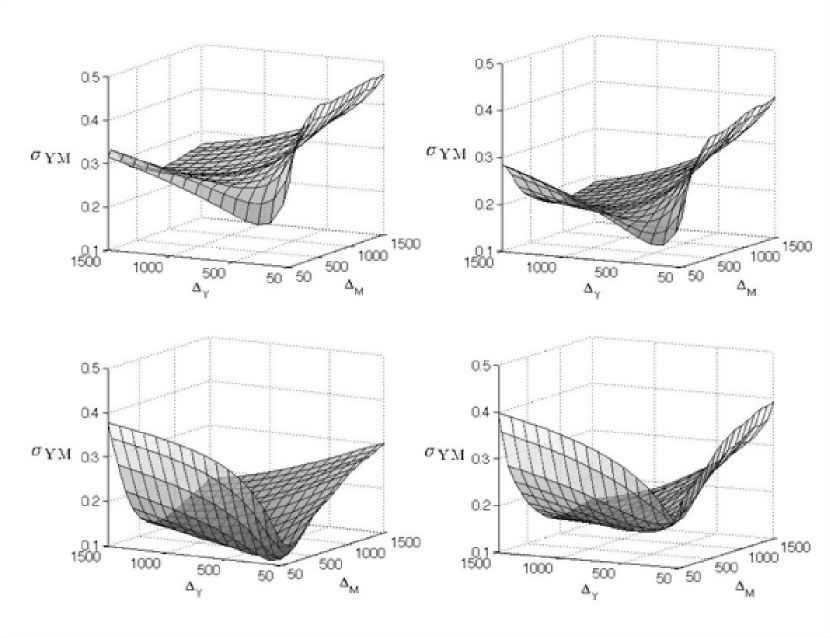
Figure 1.— The scatter, $\sigma_{\rm YM}$ (Eqn. 8), around the mass - integrated SZE relation for cluster mass measured within the radius defined by the overdensity factor $\Delta_{\rm M}$ and the integrated SZE measured within projected radius defined by $\Delta_{\rm Y}$. Each panel gives the results for one of our cluster samples: FULL (top left), NOFB (top right), BASIC (lower left) and SPH (lower right).

Figure 1 displays the scatter $\sigma_{\rm YM}$ in the $Y-M$ relation obtained for all combinations of $\Delta_{\rm Y}$ and $\Delta_{\rm M}$, for each of our cluster samples; FULL (top left), NOFB (top right), BASIC (bottom left) and SPH (bottom right). We consider first the results of the BASIC sample as it corresponds to the most simplistic case. As described in Sec 2.2, for this sample we make the simple assumption that the gas in clusters is isothermal and follows the dark matter density. Therefore, variations in the dark matter mass within $\Delta_{\rm M}$ are also reflected in the measured flux within the same overdensity, explaining the valley in the $\Delta_{\rm M}$-$\Delta_{\rm Y}$ plane along $\Delta_{\rm M}=\Delta_{\rm Y}$. This characteristic is evident in the results for all four of our cluster samples. The minimum scatter for the BASIC sample is near $\Delta=500$ for both mass and flux. This is because the temperature for these clusters was set via the $M-T_{mw}$ scaling relation, with the mass defined at $\Delta=500$.

The NOFB sample exhibits similar features to the BASIC sample, the most significant difference being the smaller rise in scatter as $\Delta_{\rm Y}$ increases at low values of $\Delta_{\rm M}$. This is straightforward to understand: assuming hydrostatic equilibrium results in gas density profiles that are less sensitive to variations in the internal mass distribution of the host dark matter halo, especially in the inner regions, than for the clusters in the BASIC sample. The gas density and temperature profiles are set by a combination of the total gravitational and kinetic energy of the gas and the surface pressure at the virial radius. We find that our recipe for star-formation has little effect on $\sigma_{\rm YM}$.

$\Delta$	$\langle f_{\rm gas}\rangle$			$\sigma_{\rm gas}/\langle f_{\rm gas}\rangle$
	FULL	NOFB	SPH	FULL	NOFB	SPH
100	0.12	0.17	0.09	0.15	0.11	0.03
200	0.11	0.16	0.09	0.15	0.11	0.04
500	0.09	0.15	0.09	0.17	0.11	0.05
1500	0.07	0.13	0.09	0.24	0.15	0.08

Table 2Mean and fractional standard deviations of the cluster gas fraction measured within four radii.

The FULL cluster sample – for which we added a prescription for energy feedback in the gas model – resembles the NOFB sample, but with uniformly greater scatter. Including feedback results in more extended (or ‘puffed out’) gas distributions, with a shallower gas density profile in the inner regions (Bode et al., 2007). Importantly, we have found that this substantially increased scatter is due to the greater variance in the gas fraction within any given overdensity. Table 2 gives the mean $\langle f_{\rm gas}\rangle$ and fractional standard deviation $\sigma_{\rm gas}/\langle f_{\rm gas}\rangle$ of the gas fraction within selected overdensities for the FULL, NOFB and SPH samples. Due to the dependence of $f_{\rm gas}$ on cluster mass in the former, we calculate these quantities for clusters in the mass range $10^{14}\leq M_{200}\leq 2\times 10^{14}h^{-1}{\rm M}_{\odot}$. Note that the mean values we measure within $R_{500}$ and $R_{100}(\approx R_{\rm vir})$ are in good agreement with the simulations of Kravtsov et al. (2005), although we measure greater scatter. For all three samples shown, the fractional scatter in $f_{\rm gas}$ increases with overdensity, most noticeably for the FULL sample. At all radii, the percentage scatter in $f_{\rm gas}$ for the FULL clusters is approximately 1.5 times greater than that for the NOFB sample and more than 3 times than that of the SPH sample. We find that $\sigma_{\rm gas}/\langle f_{\rm gas}\rangle$ increases when recalculated using lower mass clusters. Repeating this exercise for gas temperature, we find the scatter to be similar for all three models. Hence, we conclude that the scatter in $f_{\rm gas}$ for constant cluster mass is responsible for the increase in $\sigma_{\rm YM}$ over the three models in Table 2.

In the bottom right panel of Figure 1 we plot the $\sigma_{\rm YM}$ plane for the clusters extracted from the SPH simulation. The results are very similar to those of the BASIC cluster sample. The scatter is least along the valley defined by $\Delta_{\rm M}=\Delta_{\rm Y}$, rising to a maximum of $\sigma\approx 0.4$ on either side. As discussed in Sec. 2, Pearce et al. (2000), and Muanwong et al. (2001, 2002), the omission of radiative cooling in this simulation results a large central concentration of baryonic gas (compared to models that allow for cooling and star-formation) and thus in a ICM radial density profile that closely resembles that of the dark matter (see also, da Silva et al., 2004; Ettori et al., 2006). Both the BASIC and SPH samples consist of clusters with very high gas density in their centres; this is not the case for the clusters in the other two samples.

In the upper panel of Figure 2 we plot the overdensity, $\Delta_{\rm Ymin}$, at which the least-scatter measure of the integrated SZ flux is obtained for a given $\Delta_{\rm M}$. In the lower panel we plot the corresponding value of $\sigma_{\rm YM}$. The solid, dotted, dashed and dot-dashed lines represent the FULL, NOFB, BASIC and SPH cluster samples, respectively. For all four samples $\Delta_{\rm Ymin}$ increases with $\Delta_{\rm M}$, with a slope greater than one. For the FULL sample, the best measures of $M_{50}$, $M_{200}$, and $M_{500}$ are $Y_{300}$, $Y_{500}$, and $Y_{1100}$, respectively. For $\Delta_{\rm M}>700$, $\Delta_{\rm Ymin}$ appears to increase beyond the scales probed here. Performing a linear fit to this point gives $\Delta_{\rm Ymin}=1.9\Delta_{\rm M}+150$. Overall, our results show that the best measure of $M_{\Delta}$ is obtained by measuring $Y$ within a smaller area than $R_{\Delta}$.

The lower panel indicates that for the FULL and NOFB models, the scatter is least for $\Delta_{\rm M}=50$, and is roughly constant for $\Delta_{\rm M}>200$. As discussed above, much of the scatter in these models is due to variations in the baryon fraction within each radius. This source of intrinsic scatter is suppressed in the very outer regions of clusters as the baryon fraction approaches the cosmic mean. For the SPH sample, the scatter decreases with increasing $\Delta_{\rm M}$ to a constant value of 15%. For the BASIC sample, the dip in $\sigma_{\rm YM}$ at around $\Delta_{M,Y}=400$ (as noted above) is clearly evident.

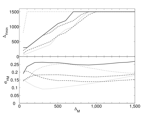
Figure 2.— (upper) The overdensity $\Delta_{\rm Ymin}$ for which the scatter $\sigma_{\rm YM}$ is least for a given $\Delta_{\rm M}$. (lower) the corresponding value of $\sigma_{\rm YM}$ for each combination of $\Delta_{\rm M}$, $\Delta_{\rm Ymin}$. Solid, dotted, dashed and dot-dashed lines correspond to the FULL, NOFB, BASIC and SPH samples respectively. The light-dashed lines are the results obtained when only clusters within a narrow concentration range are selected from the FULL sample (see Sec. 3.4). Note that where $\Delta_{\rm Ymin}$ appears to become greater than 1500, the value of $\sigma_{\rm YM}$ in the lower panel is calculated at this overdensity.

3.4. Impact of halo concentration

The concentration of a dark matter halo is normally defined as the ratio of the virial radius to the NFW scale radius, $R_{vir}/r_{s}$ and is thus a measure of the density in the halo core regions (Navarro et al., 1996, 1997). In their early studies, NFW postulated that the concentration of a halo is an indicator of the mean density of the universe at the time of its collapse (Navarro et al., 1997). Hence, present-day clusters with a high concentration will have formed early and remained undisturbed by major mergers, growing through gradual accretion and accumulation of much smaller objects. Halos with a low concentration will have had a more tumultuous recent merger history, and may still be in the process of relaxing into dynamical equilibrium (Wechsler et al., 2002, 2006; Shaw et al., 2006; Macciò et al., 2007).

There have now been many studies of distribution of halo concentration and its correlation with cluster mass (Jing, 2000; Bullock et al., 2001; Eke et al., 2001; Dolag et al., 2004; Avila-Reese et al., 2005). Most studies find that at a given redshift the distribution of halo concentrations is well described by a log-normal function of dispersion $\approx 0.22$ and mean value $<c>\approx 5$ at z=0 (Jing, 2000; Bullock et al., 2001). Halo concentration is found to decrease as a function of increasing halo mass and is well described by a power-law of slope in the range -0.14 to -0.1 (Bullock et al., 2001; Dolag et al., 2004; Shaw et al., 2006; Macciò et al., 2007). However, there is typically much scatter in this relation. One might expect to find that variations in cluster concentration (and thus central potential) will have a significant effect on the gas temperature and density profiles, and thus the $Y-M$ scaling relation. We therefore fit NFW profiles and measure the concentrations of all the halos in our samples, in order to quantitatively measure the impact of this variation.

In Fig. 3, we recalculate $\sigma_{\rm YM}$ for the FULL cluster sample, using only clusters with concentration $5.25\leq c\leq 5.75$. The clusters in this sample are thus self-similar in terms of their dark matter mass distribution. By comparing this figure with the upper-left panel of Fig. 1, it is clear that constraining halo concentration significantly changes the geometry of the $\sigma_{\rm YM}$ plane. For constant $\Delta_{\rm M}$, the scatter decreases with increasing $\Delta_{\rm Y}$. For constant $\Delta_{\rm Y}$, $\sigma_{\rm YM}$ increases slowly as $\Delta_{\rm M}$ decreases towards $\Delta_{\rm M}=500$, and then falls off rapidly in the outer regions. We have verified that similar results are obtained for different concentration bins and our three other cluster samples. On removing clusters from our sample for which the NFW profile is a poor fit, the peak at $\Delta_{\rm M}=500$ disappears, hence this feature seems to be related to clusters for which we have a poor measure of concentration.

The light-dashed line in the upper and lower panels of Figure 2 give $\Delta_{\rm Ymin}$ and the correspond scatter at each $\Delta_{\rm M}$ for the clusters in this concentration range. For all but the two outermost radii, the optimal radius within which to measure the integrated SZE appears to be less than $R_{1500}$. (Note that where $\Delta_{\rm Ymin}$ appears to become greater than 1500, the value of $\sigma_{\rm YM}$ in the lower panel is calculated at this overdensity). Motl et al. (2005) demonstrated empirically that the integrated SZE (within $R_{500}$) provides a more accurate measure of cluster mass than the central decrement, $y$. Our results suggest that variations in halo concentration (and thus central potential) between clusters of the same mass may be responsible for much of the very large scattered observed by Motl et al. (2005) in the y-M relation. Indeed, they find that $Y_{500}$ is less sensitive to mergers than $y$; it has been previously shown that concentration is strongly influenced by the dynamical state of a halo (e.g. Shaw et al., 2006; Macciò et al., 2007).

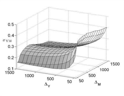
Figure 3.— The $\sigma_{\rm YM}$ plane calculated for the FULL cluster sample having included only clusters with halo concentration in the range $5.25\leq c\leq 5.75$. It is clear that the geometry of the plane is significantly altered compared to the results when all clusters are included, as shown in (the upper-left panel of) Fig. 1.

3.5. Impact of Substructure

Halo substructure is identified using the SKID algorithm of Stadel et al. (1997), with a smoothing length of $5\epsilon$, where $\epsilon$ is the spline kernel force softening length of our simulation. The minimum mass of subhalos that we resolve are $\approx 3\times 10^{11}M_{\odot}$, corresponding to 100 simulation particles. For each halo, we define the substructure fraction $f_{s}=M_{s}/M_{vir}$, where $M_{s}$ is the total subhalo mass. We find a mean value $f_{s}=0.084$ for our N-body halo sample, where we have included all subhalos with centres located within the radius $R_{50}$ of the cluster. This is in good agreement with previous studies of the substructure content on cluster mass halos (De Lucia et al., 2004; Gao et al., 2004; Gill et al., 2004; Shaw et al., 2007).

We find that, on removing all clusters with $f_{s}>0.084$ from the FULL sample, $\sigma_{YM}$ is uniformly reduced by 10%. Taking the sample quartile with the lowest substructure fraction ($f_{s}<0.050$) we find the average decrease in $\sigma_{YM}$ is 20% (e.g. at $\Delta_{\rm Y}=\Delta_{\rm M}=100$, $\sigma_{\rm YM}$ is reduced from 0.30 to 0.25). Taking the quartile with the highest substructure fraction ($f_{s}>0.010$) increases $\sigma_{\rm YM}$ by 32% (compared to the result for the entire sample). Note that in all cases the geomentry of the $\sigma_{\rm YM}$ plane does not change significantly from that shown in the upper-left panel of Fig. 1.

Overall, we find that substructure accounts for approximately a fifth of the total amount of scatter in the $Y-M$ relation, but – unlike the variations in halo concentration – does not strongly effect the dependence of $\sigma_{\rm YM}$ on the combination of $\Delta_{\rm Y}$ and $\Delta_{\rm M}$.

4. Impact of Projection Effects on the $Y-M$ relation

Taking the standard definition of cluster mass, $M_{200}$, we have established that the intrinsic scatter in the $Y-M_{200}$ scaling relation is least when $Y$ is measured within $R_{500}$ ($\approx 0.66{\rm R}_{200}$). Assuming that $\sigma_{\rm YM}$ does not change significantly with redshift, for a cluster at redshift $z$ this radius translates to an optimal angular radius, $\theta_{opt}$, within which one can obtain the least-scatter estimate of cluster mass through an SZE measurement. However in order to make a useful estimate of $\theta_{\rm opt}$, we must also account for the impact of the SZ background – the superposition of faint fore- and background clusters along the line of sight – when measuring the integrated SZ flux of a cluster within some angular radius $\theta$.

Recently, Holder et al. (2007) investigated the confusion in cluster SZE flux measurements due to the SZ background using a sample of sky maps constructed to represent a range in $\sigma_{8}$ of 0.6–1. Intracluster gas was assumed to follow the analytic model of McCarthy et al. (2003). They found that the mass scale below which the $rms$ fractional errors in flux measurements become less than 20% occurs at just above $10^{14}h^{-1}{\rm M}_{\odot}$, although this is sensitively dependent on $\sigma_{8}$ and increases with decreasing redshift. Hallman et al. (2007) explored the contribution of both gas in low mass ($<5\times 10^{13}{\rm M}_{\odot}$) halos and gas outside of cluster environments on the SZE signature of resolvable clusters, using lightcones constructed from an adiabatic hydro simulation. They find that the integrated background SZE makes up between 4% and 12% of the total cluster signal, depending on the beam size and sensitivity of a survey, although these values are averaged over a range of cluster masses. Both these studies concentrated on the SZ background as the main source of scatter in SZ cluster mass measurements. In this Section, we combine the intrinsic scatter in the $Y-M$ relation due to internal variations between clusters ($\sigma_{\rm YM}$) with that due to confusion with the SZ background, in order to obtain the optimal angular radius $\theta_{opt}$ within which the integrated SZE can best be obtained for a cluster of given mass and redshift. Henceforth, we fix our definition of cluster mass to the standard definition, $M_{200}$.

For this purpose, we use the redshift range $0\leq z\leq 1.5$ of a lightcone constructed from an N-body simulation with the same cosmology as that used in the previous section, but with lower mass resolution (particle mass $m_{p}=1.22\times 10^{11}\,h^{-1}{\rm M}_{\odot}$). The lower resolution was enforced due to the amount of disk space required to store the lightcone over an octant ($\approx 5250$ square degrees) out to high redshift, and the computing time required to analyze determine the gas distribution within each halo with the full gas model (including star formation and feedback) within this volume.

We proceed in the following manner. First, we measure the mean $\langle Y_{bck}\rangle$ and standard deviation $\delta_{bck}$ of the background integrated SZE within a circular aperture of radius $\theta$ centred around each cluster in a sample of images generated from the lightcone. We do this for a range of angular radii, varying $\theta$ from 0.5 to 15 arcminutes. We then obtain the total scatter in the integrated SZE measured within $\theta$ for a cluster of mass $M_{200}$ at a redshift $z$ by combining in quadrature the scatter due to variations in the background flux with that due to variations in the internal properties of clusters, as measured in Sec. 3.

To measure $\langle Y_{bck}\rangle$ and $\delta_{bck}$ we randomly select a sample of 100 clusters, each with mass $M_{200}\geq 10^{14}h^{-1}{\rm M}_{\odot}$, over a redshift range $0.2\leq z\leq 1$ from the lightcone. For each cluster we generate two images, one including and one omitting all the foreground and background clusters within a one degree radius around the cluster. We then remove the latter from the former, leaving just an image of the interlopers. We wish to investigate the impact of the SZ background due to dim clusters along the line of sight, therefore we also remove all clusters with an SZ signal to noise $\geq 5$ from the images, where $Y$ is measured within $\theta(R_{200},z)$ and we assume an instrument noise of $10\mu$K. These clusters are then removed in the following manner. First, the central pixel of the interloper is identified and the flux $y_{max}$ recorded. Next, a beta model of the form

$$y(\theta)=y_{max}(1+\theta^{2}/\theta_{c}^{2})^{-0.5}$$ (9)

is deducted from the image, where $\theta_{c}\approx R_{vir}/20D_{a}$, and $R_{vir}$ and the angular diameter distance, $D_{a}$, are taken directly from our lightcone halo catalog (we remove the cluster signal out to the angular size corresponding to the virial radius of each cluster).

Note that we do not add the primary CMB signal or other sources of ‘noise’ – radio point sources, instrumental noise, galactic dust emission and atmospheric emission (see, for example, Sehgal et al., 2007) – into these images. In a subsequent paper (Shaw & Holder, in preparation) we will investigate in more depth the accuracy with which matched-filtering schemes (e.g. Melin et al., 2006) can measure clusters masses, incorporating some of these effects. Here we focus solely on sources of scatter in the $Y-M$ relation that are due to variations in the internal properties and spatial distributions of clusters, and thus cannot be suppressed.

We measure the mean and standard deviation of the background integrated SZE at each value of $\theta$ over the selected cluster sample. The results are displayed in Fig. 4. The crosses represent the mean integrated flux $\langle{\rm Y_{bck}}\rangle$ within $\theta$. The circles represent the standard deviation $\delta_{\rm bck}$ around the mean for each $\theta$. We find that both are well described by a power-law, with

$$\langle{\rm Y_{bck}}\rangle=10^{-5.66}\theta^{1.85}$$ (10)

and

$$\delta_{\rm bck}=10^{-5.4}\theta^{1.61}\;,$$ (11)

plotted as solid and dashed lines, respectively. We note that both $\langle{\rm Y_{bck}}\rangle$ and $\delta_{\rm bck}$ are dependent on the matter power spectrum and thus on the values of $\Omega_{M}$ and $\sigma_{8}$ (as demonstrated by Holder et al., 2007) and therefore the values measured here are only relevant for the cosmology assumed by our simulation.

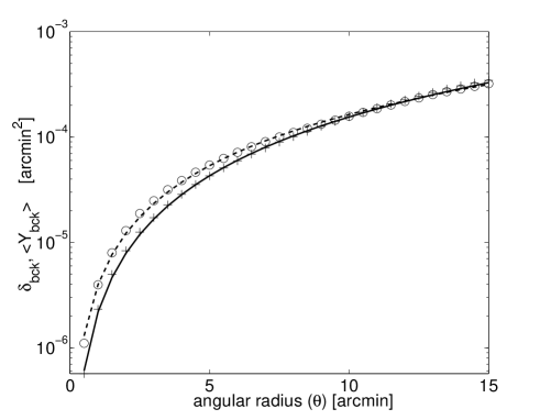
Figure 4.— The mean ($\langle{\rm Y_{bck}}\rangle$, crosses) and standard deviation ($\delta_{\rm bck}$ , circles) of the background SZE flux measured within an angular region of radius $\theta$ centred around each bright cluster in our sample of images, due to dim, unresolvable clusters (see text). Solid and dashed lines give power-law fits to the results, as given in Eqns. 10 and 11.

Using Equations 10 and 11, and the fitted values for the $Y_{\Delta}-M_{200}$ scaling relations measured in Section. 3, we are now able to calculate the mean total flux that would be measured within an angular radius $\theta(\Delta_{\rm Y},z)$ for a cluster of mass $M_{200}$ at redshift $z$:

$$Y_{tot}(M_{200},\theta)=\langle Y_{bck}(\theta)\rangle+Y_{\rm clus}(M_{200},\theta,z)\;,$$ (12)

where

$$Y_{\rm clus}(M_{200},\theta,z)=\frac{E(z)^{3/2}}{d^{2}_{A}(z)}10^{A(\Delta)}\left(\frac{M_{200}}{10^{14}h^{-1}{\rm M}_{\odot}}\right)^{\alpha(\Delta)}$$ (13)

and $\theta=\theta(\Delta,z)$ is the angular radius corresponding to a cluster with radius $R_{\Delta}$ at angular diameter distance $d_{A}(z)$ (note the units of $Y_{\rm clus}$ are arcmin², see Eqn. 3). $A(\Delta)$ and $\alpha(\Delta)$ are the corresponding normalisation index and slope obtained for the $Y_{\Delta}-M_{200}$ relation as measured in Section 3. The radius at a given $\Delta$ is calculated at redshift $z$ by relating $R_{\Delta}$ to $R_{200}$ through the NFW profile. We use the mass-concentration fitting formula of Dolag et al. (2004) to calculate the mean concentration for a cluster of mass $M_{200}$ at each cluster redshift. We assume that the slope and normalisation of the $Y-M$ relation are independent of redshift (having accounted for the hubble scaling, $E(z)$). Nagai (2006) have found this to be the case for a simulated sample of clusters encompassing a redshift range $0\geq z\geq 2$.

We can calculate the total scatter in $Y_{tot}(\theta,M,z)$ by combining the scatter in the mean background flux with the intrinsic scatter in the $Y-M$ relation $\sigma_{\rm YM}(\Delta_{\rm Y})$;

$$\sigma_{tot}(\theta,M,z)=\frac{(\delta_{bck(\theta)}^{2}+\delta_{clus}^{2})^{\frac{1}{2}}}{Y_{\rm tot}}\;,$$ (14)

where

$$\delta_{clus}=Y_{\rm clus}\sigma_{\rm YM}(\Delta_{\rm Y})\;,$$ (15)

thus converting the fractional scatter $\sigma_{\rm YM}\approx\delta_{\rm clus}/Y_{\rm clus}$, to an absolute value.

Figure 5 demonstrates the dependence of $\sigma_{tot}$ (solid lines) on angular radius for clusters of mass $10^{14}h^{-1}{\rm M}_{\odot}$ and $2\times 10^{14}h^{-1}{\rm M}_{\odot}$, at redshifts $z=0.5$ and $1$. Also plotted are $\delta_{\rm clus}/Y_{\rm tot}$ (dashed) and $\delta_{\rm bck}/Y_{\rm tot}$ (dotted). The minimum of the dashed line corresponds to angular radius subtending $R_{500}$ for each cluster mass and redshift. For a $10^{14}h^{-1}{\rm M}_{\odot}$ cluster (left panels), including the SZE background moves the optimal value of $\theta$ to a lower angular radii than that predicted by the intrinsic cluster scatter $\delta_{\rm clus}$ alone. At z = 0.5, this decrease is 0.4 arcminutes, and at z = 1 it is 0.25 arcminutes. At higher redshifts, the cluster subtends a smaller angular region and thus the impact of the background flux is lessened. This is also the case as cluster mass is increased. The right panels of Figure 5 demonstrate that, for a $2\times 10^{14}h^{-1}{\rm M}_{\odot}$ cluster, the background flux is small compared to the cluster signal, and therefore $\delta_{\rm bck}$ does not change $\theta$ significantly. Hence, for clusters of mass $M_{200}\geq 2\times 10^{14}h^{-1}{\rm M}_{\odot}$ variations in the SZE background are negligible compared to the intrinsic scatter in $Y$ due to variations in the internal properties of clusters.

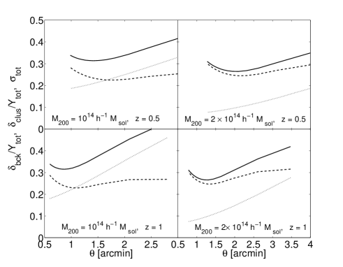
Figure 5.— (solid lines) The total scatter $\sigma_{\rm tot}$ (Eqn. 14) in the $Y-M$ relation for $Y$ measured within angular radius $\theta$ for a $10^{14}h^{-1}{\rm M}_{\odot}$ (left panels) and $2\times 10^{14}h^{-1}{\rm M}_{\odot}$ (right) cluster at redshifts 0.5 (upper panels) and 1 (lower). The dashed lines give the fractional variation in the intrinsic scatter ($\delta_{\rm clus}/Y_{\rm tot}$, Eqn. 15), the dotted lines give the fractional variation in the SZE background ($\delta_{\rm bck}/Y_{\rm tot}$), within $\theta$ for each cluster mass.

Finally, in Fig. 6 we plot the optimal angle $\theta_{\rm opt}(z)$ within which the integrated SZ signal provides the least scatter measure of $M_{200}$ as a function of redshift. The solid, dotted, dashed and dot-dashed lines correspond to 1,2,5 and 10 $\times 10^{14}h^{-1}{\rm M}_{\odot}$ clusters respectively. Thus $\theta_{\rm opt}(z=0.5)$ varies between 1.5 and 4 arcminutes as mass increases. For $z>1$, all clusters have an optimal angular radius less than 2 arcminutes.

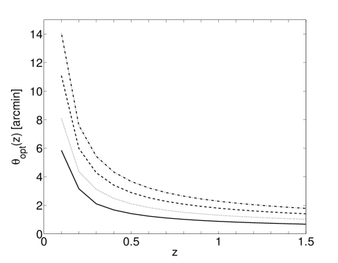
Figure 6.— The optimal angle $\theta_{\rm opt}$ within which SZE flux can be measured for a cluster of mass $10^{14}$ (solid line), $2\times 10^{14}$ (dotted), $5\times 10^{14}$ (dashed) and $10^{15}$ (dot-dashed) $h^{-1}{\rm M}_{\odot}$ to give the last scatter (intrinsic plus projected) in the $Y-M$ relation cluster at redshift $z$.

5. Discussion and Conclusions

The Sunyaev-Zel’dovich effect is one of the most promising means for precise determination of cosmological parameters because the mapping between the integrated SZ flux and cluster mass is expected to have very low intrinsic scatter. Thus there is a need for concerted investigation into the origins and character of the scatter that is present in this relation, and how the scatter may be reduced.

In this paper, we have presented a detailed analysis of the intrinsic scatter in the integrated SZE–cluster mass ($Y-M$) relation, using large simulated cluster samples generated from a semi-analytic model of intracluster gas applied to the lightcone output of a high resolution N-body simulation, and also clusters extracted directly from an adiabatic SPH simulation. In particular, the main aims of this study were to investigate the impact on this relation of:

• the choice of how cluster mass is defined and the region within which the integrated SZE is measured; i.e. the impact of measuring these quantities within different radii $R_{\Delta}$, where $\Delta$ is the overdensity relative to the critical density,

• incorporating energy feedback due to supernovae and AGN outflows into the cluster gas model,

• variations in host halo concentration and substructure populations,

• the error in SZ flux measurements due to confusion with unresolvable (i.e. low Y) clusters along the line of sight.

To assess the impact of the definition of $Y$ and $M$, we measure both quantities within radii corresponding to a range of overdensities between $\Delta=50$ and $1500$. We measure the slope, normalisation and scatter in the ${\rm Y_{\Delta}-M_{\Delta}}$ relation using all combinations of $\Delta_{Y}$ and $\Delta_{M}$ (not just $\Delta_{Y}=\Delta_{M}$). The effect of energy feedback on the scatter is investigated by generating three realisations of our gas model, respectively including and omitting energy feedback and a toy model in which the gas is isothermal and follows the dark matter density. Each sample contained 1267 clusters. For comparison, we also take a sample of 212 clusters from the output of an adiabatic simulation (Muanwong et al., 2001). For each sample, we also measure the concentration and fraction of mass contained in substructure of the host dark matter halos.

Finally, we address the issue of the SZE background using the full lightcone output of our N-body simulation. We measure the SZE background due to low mass systems within a range of solid angles, combining the scatter in the background flux with the intrinsic scatter in the $Y-M$ relation (within a given angular radius) to determine the optimal angular size within which the scatter in the measured $Y$ for a cluster of given mass and redshift is least. Our results are summarized below.

1. Scatter in the intrinsic $Y-M$ relation is least when cluster mass is defined within as large a radius as possible (to a maximum of $R_{50}$ in this study) and the integrated SZE is measured in the range $R_{500}\leq R_{\Delta}\leq R_{300}$. For $M_{50}$ the scatter is least for $Y_{300}$. For $M_{200}$, the scatter is least for $Y_{500}$. In general, the least scatter measure of $Y$ is always obtained within a smaller radii than that at which the mass is defined. We find that the best overdensity within which to measure Y is given by $\Delta_{\rm Y}=1.9\Delta_{M}+150$.

2. Inclusion of energy feedback in our gas model significantly increases the intrinsic scatter in the $Y-M$ relation for all combinations of $\Delta_{\rm M}$ and $\Delta_{\rm Y}$. We find that this is due to significantly larger variations in the gas mass fraction within any radius than in our other cluster samples.

3. Variations in host halo concentration/central potential (for clusters of the same mass), and the resulting impact on the cluster gas distribution, provide a reason as to why the integrated SZE provides a tighter proxy for cluster mass than the central decrement. Constraining halo concentration (i.e. selecting only clusters within a narrow concentration range) changes the $Y-M$ relation for high $\Delta_{\rm Y}$ so that the least scatter measure of $M_{\Delta}$ is obtained by measuring the integrated SZE within a radius $R\leq R_{1500}$, the minimum radius probed in this study.

4. Substructure increases scatter uniformly for all combinations of $\Delta_{\rm M}$ and $\Delta_{\rm Y}$. Removing clusters with large amounts of substructure reduces scatter in the $Y-M$ relation by up to 20%.

5. The mean integrated SZE around a cluster due to low-mass foreground and background clusters along the line of sight scales with angular radius $\langle Y_{bck}\rangle=10^{-5.66}\theta^{1.85}$, and the standard deviation as $\delta_{bck}=10^{-5.4}\theta^{1.61}$.

6. For cluster of mass $M_{200}\geq 2\times 10^{14}h^{-1}{\rm M}_{\odot}$, the optimal angular radius within which one should measure the SZE so as to obtain the tightest scaling with cluster mass ($M_{200}$) is just the angle subtending $R_{500}$ at the cluster redshift (the radius at which intrinsic scatter due to variations in internal cluster properties is least). Below this mass, the magnitude and variance of the SZE background relative to the cluster signal reduces the optimal angular radius (e.g by 0.4 arcminutes at z = 0.5 for a $10^{14}h^{-1}{\rm M}_{\odot}$ cluster). In addition, we have provided a chart (Fig. 6) giving the optimal angular size for measuring clusters masses using the SZE for a range of masses and redshifts.

One important result of this study is that we measure there to be at least 20% intrinsic scatter in the $Y-M$ relation due variations in the internal properties of clusters alone. When mass and SZ flux are measured at $R_{200}$, the scatter is just above 25%. This is higher than the 10-15% scatter that has been quoted by previous authors using small samples of clusters extracted from highly sophisticated simulations including complex gas physics (e.g. Nagai, 2006) or larger samples of less-well resolved clusters (da Silva et al., 2004; Motl et al., 2005; Hallman et al., 2007). As noted above, we have found that much of the scatter we measure is due to the variations in the gas mass fraction between clusters of similar mass, an effect that is greatly enhanced by the inclusion of energy feedback into our models. However, observational measures of the gas fraction from X-ray studies of bright clusters certainly seem to suggest that there is indeed much variation in this quantity between clusters (Vikhlinin et al., 2006; Zhang et al., 2007). Nevertheless, we intend to perform a rigorous comparison between the predictions of our gas model and the results of hydrodynamical simulations within the near future.

We have shown that a significant fraction of the scatter in the $Y-M$ scaling relation is due to variations in the host halo properties, specifically in concentration and substructure populations. Our results suggest that, if all halos at a given mass had the same merger history, then the central SZE decrement might provide the best measure of halo mass. However, the variations in cluster structure due to mergers greatly and preferentially increase the scatter in Y when measured only within the central regions ($R_{1500}$), hence it becomes necessary to integrate to larger radii. We have shown that there is a limit to how far out one should go, however, before projection effects due to dim, unresolvable clusters begin to significant effect SZE flux measurements.

We have not investigated the impact of morphology and environment in this study, which may also play significant roles. We leave this to future work. Furthermore, our gas model is not able to accurately account for some of the complex physical processes such as shock heating during mergers and cooling in cluster cores, which will certainly introduce additional scatter in scaling relations (McCarthy et al., 2004; O’Hara et al., 2006; Poole et al., 2007).

Finally, several studies have demonstrated there to be significant errors in extracting the correct value of $Y$ from synthetic sky maps due to CMB confusion, instrument noise, the effect of galactic dust emission, diffuse gas outside of clusters and radio point sources, and systematic effects in the cluster identification algorithm utilized (Melin et al., 2006; Hallman et al., 2007; Juin et al., 2007; Schäfer et al., 2006a, b; Pires et al., 2006; Sehgal et al., 2007). Combined with the intrinsic scatter in the $Y-M$ as measured here, it is clear that there is still much work to be done to enable accurate estimation of cluster masses and thus achieve the tight cosmological constraints that are envisaged from SZ cluster surveys.

6. ACKNOWLEDGMENTS

This work supported by the Natural Sciences and Engineering Research Council (Canada) through the Discovery Grant Awards to GPH. GPH would also like to acknowledge support from the Canadian Institute for Advance Research and the Canada Research Chairs Program. This research was facilitated by allocations of time on the COSMOS supercomputer at DAMTP in Cambridge, a UK-CCC facility supported by HEFCE and PPARC, and advanced computing resources from the Pittsburgh Supercomputing Center and the National Center for Supercomputing Applications. In addition, computational facilities at Princeton supported by NSF grant AST-0216105 were used, as well as high performance computational facilities supported by Princeton University under the auspices of the Princeton Institute for Computational Science and Engineering (PICSciE) and the Office of Information Technology (OIT). We would also like to thank A. Evrard and J.P. Ostriker for helpful discussions.

References

- Ascasibar et al. (2006) Ascasibar, Y., Sevilla, R., Yepes, G., Müller, V., & Gottlöber, S. 2006, MNRAS, 371, 193
- Avila-Reese et al. (2005) Avila-Reese, V., Colín, P., Gottlöber, S., Firmani, C., & Maulbetsch, C. 2005, ApJ, 634, 51
- Bahcall & Fan (1998) Bahcall, N. & Fan, X. 1998, ApJ, 504, 1
- Balogh et al. (1999) Balogh, M. L., Babul, A., & Patton, D. R. 1999, MNRAS, 307, 463
- Barbosa et al. (1996) Barbosa, D., Bartlett, J., Blanchard, A., & Oukbir, J. 1996, A&A, 314, 13
- Benson et al. (2004) Benson, B. A., Church, S. E., Ade, P. A. R., Bock, J. J., Ganga, K. M., Henson, C. N., & Thompson, K. L. 2004, ApJ, 617, 829
- Birkinshaw (1999) Birkinshaw, M. 1999, Physics Reports, 310, 97
- Bode et al. (2007) Bode, P., Ostriker, J. P., Weller, J., & Shaw, L. 2007, ApJ, 663, 139
- Borgani et al. (2005) Borgani, S., Finoguenov, A., Kay, S. T., Ponman, T. J., Springel, V., Tozzi, P., & Voit, G. M. 2005, MNRAS, 361, 233
- Bryan & Norman (1998) Bryan, G. L. & Norman, M. L. 1998, ApJ, 495, 80
- Bullock et al. (2001) Bullock, J. S., Kolatt, T. S., Sigad, Y., Somerville, R. S., Kravtsov, A. V., Klypin, A. A., Primack, J. R., & Dekel, A. 2001, MNRAS, 321, 559
- Carlstrom et al. (2002) Carlstrom, J. E., , Holder, G. P., & Reese, E. D. 2002, ARA&A, 40, 643
- Cole & Lacey (1996) Cole, S. & Lacey, C. 1996, MNRAS, 281, 716
- Couchman et al. (1995) Couchman, H. M. P., Thomas, P. A., & Pearce, F. R. 1995, ApJ, 452, 797
- da Silva et al. (2004) da Silva, A. C., Kay, S. T., Liddle, A. R., & Thomas, P. A. 2004, MNRAS, 348, 1401
- De Lucia et al. (2004) De Lucia, G., Kauffmann, G., Springel, V., White, S. D. M., Lanzoni, B., Stoehr, F., Tormen, G., & Yoshida, N. 2004, MNRAS, 348, 333
- Dolag et al. (2004) Dolag, K., Bartelmann, M., Perrotta, F., Baccigalupi, C., Moscardini, L., Meneghetti, M., & Tormen, G. 2004, A&A, 416, 853
- Eke et al. (1996) Eke, V. R., Cole, S., & Frenk, C. S. 1996, MNRAS, 282, 263
- Eke et al. (1998a) Eke, V. R., Cole, S., Frenk, C. S., & Patrick Henry, J. 1998a, MNRAS, 298, 1145
- Eke et al. (1998b) Eke, V. R., Navarro, J. F., & Frenk, C. S. 1998b, ApJ, 503, 569
- Eke et al. (2001) Eke, V. R., Navarro, J. F., & Steinmetz, M. 2001, ApJ, 554, 114
- Ettori et al. (2006) Ettori, S., Dolag, K., Borgani, S., & Murante, G. 2006, MNRAS, 365, 1021
- Evrard et al. (2007) Evrard, A. E., Bialek, J., Busha, M., White, M., Habib, S., Heitmann, K., Warren, M., Rasia, E., Tormen, G., Moscardini, L., Power, C., Jenkins, A. R., Gao, L., Frenk, C. S., Springel, V., White, S. D. M., & Diemand, J. 2007, ArXiv Astrophysics e-prints
- Evrard & Henry (1991) Evrard, A. E. & Henry, J. P. 1991, ApJ, 383, 95
- Gao et al. (2004) Gao, L., White, S. D. M., Jenkins, A., Stoehr, F., & Springel, V. 2004, MNRAS, 355, 819
- Gill et al. (2004) Gill, S. P. D., Knebe, A., Gibson, B. K., & Dopita, M. A. 2004, MNRAS, 351, 410
- Haiman et al. (2001) Haiman, Z., Mohr, J. J., & Holder, G. P. 2001, ApJ, 553, 545
- Hallman et al. (2007) Hallman, E. J., O’Shea, B. W., Burns, J. O., Norman, M. L., Harkness, R., & Wagner, R. 2007, ArXiv e-prints, 704
- Holder et al. (2007) Holder, G., McCarthy, I. G., & Babul, A. 2007, ArXiv Astrophysics e-prints
- Hu (2003) Hu, W. 2003, Phys. Rev. D, 67, 081304
- Jing (2000) Jing, Y. P. 2000, ApJ, 535, 30
- Juin et al. (2007) Juin, J. B., Yvon, D., Réfrégier, A., & Yèche, C. 2007, A&A, 465, 57
- Kaiser (1991) Kaiser, N. 1991, ApJ, 383, 104
- Kosowsky (2003) Kosowsky, A. 2003, New Astronomy Review, 47, 939
- Kravtsov et al. (2002) Kravtsov, A. V., Klypin, A., & Hoffman, Y. 2002, ApJ, 571, 563
- Kravtsov et al. (2005) Kravtsov, A. V., Nagai, D., & Vikhlinin, A. A. 2005, ApJ, 625, 588
- Lacey & Cole (1993) Lacey, C. & Cole, S. 1993, MNRAS, 262, 627
- Lahav et al. (1991) Lahav, O., Lilje, P. B., Primack, J. R., & Rees, M. J. 1991, MNRAS, 251, 128
- Lima & Hu (2004) Lima, M. & Hu, W. 2004, Phys. Rev. D, 70, 043504
- Lima & Hu (2005) —. 2005, Phys. Rev. D, 72, 043006
- Lin et al. (2003) Lin, Y.-T., Mohr, J. J., & Stanford, S. A. 2003, ApJ, 591, 749
- Macciò et al. (2007) Macciò, A. V., Dutton, A. A., van den Bosch, F. C., Moore, B., Potter, D., & Stadel, J. 2007, MNRAS, 378, 55
- Majumdar & Mohr (2003) Majumdar, S. & Mohr, J. J. 2003, ApJ, 585, 603
- McCarthy et al. (2003) McCarthy, I. G., Babul, A., Holder, G. P., & Balogh, M. L. 2003, ApJ, 591, 515
- McCarthy et al. (2004) McCarthy, I. G., Balogh, M. L., Babul, A., Poole, G. B., & Horner, D. J. 2004, ApJ, 613, 811
- Melin et al. (2006) Melin, J.-B., Bartlett, J. G., & Delabrouille, J. 2006, A&A, 459, 341
- Morandi et al. (2007) Morandi, A., Ettori, S., & Moscardini, L. 2007, MNRAS, 379, 518
- Motl et al. (2005) Motl, P. M., Hallman, E. J., Burns, J. O., & Norman, M. L. 2005, ApJ, 623, L63
- Muanwong et al. (2006) Muanwong, O., Kay, S. T., & Thomas, P. A. 2006, ApJ, 649, 640
- Muanwong et al. (2002) Muanwong, O., Thomas, P. A., Kay, S. T., & Pearce, F. R. 2002, MNRAS, 336, 527
- Muanwong et al. (2001) Muanwong, O., Thomas, P. A., Kay, S. T., Pearce, F. R., & Couchman, H. M. P. 2001, ApJ, 552, L27
- Nagai (2006) Nagai, D. 2006, ApJ, 650, 538
- Nagamine et al. (2006) Nagamine, K., Ostriker, J. P., Fukugita, M., & Cen, R. 2006, ApJ, 653, 881
- Navarro et al. (1996) Navarro, J. F., Frenk, C. S., & White, S. D. M. 1996, ApJ, 462, 563
- Navarro et al. (1997) —. 1997, ApJ, 490, 493
- O’Hara et al. (2006) O’Hara, T. B., Mohr, J. J., Bialek, J. J., & Evrard, A. E. 2006, ApJ, 639, 64
- Ostriker et al. (2005) Ostriker, J. P., Bode, P., & Babul, A. 2005, ApJ, 634, 964
- Pearce & Couchman (1997) Pearce, F. R. & Couchman, H. M. P. 1997, New Astronomy, 2, 411
- Pearce et al. (2000) Pearce, F. R., Thomas, P. A., Couchman, H. M. P., & Edge, A. C. 2000, MNRAS, 317, 1029
- Perlmutter et al. (1999) Perlmutter, S., Aldering, G., Goldhaber, G., Knop, R., Nugent, P., Castro, P., Deustua, S., Fabbro, S., Goobar, A., Groom, D. E., Hook, I. M., Kim, A. G., Kim, M., Lee, J., Nunes, N., Pain, R., Pennypacker, C., Quimby, R., Lidman, C., Ellis, R., Irwin, M., McMahon, R., Ruiz-Lapuente, P., Walton, N., Schaefer, B., Boyle, B., Filippenko, A., Matheson, T., Fruchter, A., Panagia, N., Newberg, H. J. M., & Couch, W. 1999, ApJ, 517, 565
- Pires et al. (2006) Pires, S., Juin, J. B., Yvon, D., Moudden, Y., Anthoine, S., & Pierpaoli, E. 2006, A&A, 455, 741
- Poole et al. (2007) Poole, G. B., Babul, A., McCarthy, I. G., Fardal, M. A., Bildfell, C. J., Quinn, T., & Mahdavi, A. 2007, MNRAS, 380, 437
- Romeo et al. (2006) Romeo, A. D., Sommer-Larsen, J., Portinari, L., & Antonuccio-Delogu, V. 2006, MNRAS, 373, 1648
- Ruhl (2004) Ruhl, J., e. a. 2004, in Presented at the Society of Photo-Optical Instrumentation Engineers (SPIE) Conference, Vol. 5498, Millimeter and Submillimeter Detectors for Astronomy II., ed. C. M. Bradford, P. A. R. Ade, J. E. Aguirre, J. J. Bock, M. Dragovan, L. Duband, L. Earle, J. Glenn, H. Matsuhara, B. J. Naylor, H. T. Nguyen, M. Yun, & J. Zmuidzinas, 11–29
- Schäfer et al. (2006a) Schäfer, B. M., Pfrommer, C., Bartelmann, M., Springel, V., & Hernquist, L. 2006a, MNRAS, 370, 1309
- Schäfer et al. (2006b) Schäfer, B. M., Pfrommer, C., Hell, R. M., & Bartelmann, M. 2006b, MNRAS, 370, 1713
- Schmidt et al. (1998) Schmidt, B. P., Suntzeff, N. B., Phillips, M. M., Schommer, R. A., Clocchiatti, A., Kirshner, R. P., Garnavich, P., Challis, P., Leibundgut, B., Spyromilio, J., Riess, A. G., Filippenko, A. V., Hamuy, M., Smith, R. C., Hogan, C., Stubbs, C., Diercks, A., Reiss, D., Gilliland, R., Tonry, J., Maza, J. e., Dressler, A., Walsh, J., & Ciardullo, R. 1998, ApJ, 507, 46
- Sehgal et al. (2007) Sehgal, N., Trac, H., Huffenberger, K., & Bode, P. 2007, ApJ, 664, 149
- Shaw et al. (2006) Shaw, L. D., Weller, J., Ostriker, J. P., & Bode, P. 2006, ApJ, 646, 815
- Shaw et al. (2007) —. 2007, ApJ, 659, 1082
- Sijacki & Springel (2006) Sijacki, D. & Springel, V. 2006, ArXiv Astrophysics e-prints
- Solanes et al. (2005) Solanes, J. M., Manrique, A., González-Casado, G., & Salvador-Solé, E. 2005, ApJ, 628, 45
- Spergel et al. (2007) Spergel, D. N., Bean, R., Doré, O., Nolta, M. R., Bennett, C. L., Dunkley, J., Hinshaw, G., Jarosik, N., Komatsu, E., Page, L., Peiris, H. V., Verde, L., Halpern, M., Hill, R. S., Kogut, A., Limon, M., Meyer, S. S., Odegard, N., Tucker, G. S., Weiland, J. L., Wollack, E., & Wright, E. L. 2007, ApJS, 170, 377
- Stadel et al. (1997) Stadel, J., Katz, N., Weinberg, D. H., & Hernquist, L. 1997, www-hpcc.astro.washington.edu/tools/skid.html
- Sunyaev & Zel’dovich (1972) Sunyaev, R. A. & Zel’dovich, Y. B. 1972, Comments Astrophys. Space Phys., 4, 173
- Thomas & Couchman (1992) Thomas, P. A. & Couchman, H. M. P. 1992, MNRAS, 257, 11
- Thomas et al. (2002) Thomas, P. A., Muanwong, O., Kay, S. T., & Liddle, A. R. 2002, MNRAS, 330, L48
- Vikhlinin et al. (2006) Vikhlinin, A., Kravtsov, A., Forman, W., Jones, C., Markevitch, M., Murray, S. S., & Van Speybroeck, L. 2006, ApJ, 640, 691
- Voevodkin & Vikhlinin (2004) Voevodkin, A. & Vikhlinin, A. 2004, ApJ, 601, 610
- Wechsler et al. (2002) Wechsler, R. H., Bullock, J. S., Primack, J. R., Kravtsov, A. V., & Dekel, A. 2002, ApJ, 568, 52
- Wechsler et al. (2006) Wechsler, R. H., Zentner, A. R., Bullock, J. S., Kravtsov, A. V., & Allgood, B. 2006, ApJ, 652, 71
- Weller et al. (2001) Weller, J., Battye, R., & Kneissl, R. 2001, Phys. Rev. Lett., 88, 231301
- White (2001) White, M. 2001, A&A, 367, 27
- White et al. (2002) White, M., Hernquist, L., & Springel, V. 2002, ApJ, 579, 16
- Zhang et al. (2007) Zhang, Y.-Y., Finoguenov, A., Böhringer, H., Kneib, J.-P., Smith, G. P., Czoske, O., & Soucail, G. 2007, A&A, 467, 437