Determination of spin polarization in InAs/GaAs self-assembled quantum dots

Abstract

The spin polarization of electrons trapped in InAs self-assembled quantum dot ensembles is investigated. A statistical approach for the population of the spin levels allows one to infer the spin polarization from the measure values of the addition energies. From the magneto-capacitance spectroscopy data, the authors found a fully polarized ensemble of electronic spins above 10 T when $\mathbf{B}\parallel[001]$ and at 2.8 K. Finally, by including the g-tensor anisotropy the angular dependence of spin polarization with the magnetic field $\mathbf{B}$ orientation and strength could be determined.

Spin polarization in quantum dots (QDs) is a desirable measurement for a complete characterization of the magnetic response of these systems. The assessment of this quantity has an important impact on the usefulness of QDs for quantum computing processing schemes. Recently, there has been several experiments relying on the optical selection rules for the determination of spin polarization in QD ensembles gupta ; chye ; loffler ; li ; lombez ; gundogdu ; itskos . State preparation and measurement with circularly polarized excitation gupta , spin injection with ferromagnetic contacts into light emitting diodes chye ; loffler ; li ; lombez , time and polarization resolved photoluminescence gundogdu and oblique Hanle effect itskos have been used in order to characterize spin polarization. Yet, in order to explain the inferred polarization, theoretical results point out that one needs to take into account the hole polarization in the final result pryor ; hawrylak .

In contrast to optical schemes, electrical readout of the electronic spins orientation does not require any knowledge of hole polarization, depending only on spin-to-charge conversion vandersypen . Here we perform magneto-capacitance measurements of QDs embedded in a Metal-Insulator-Semiconductor (MIS) capacitor structure. The amount of polarization was inferred by measuring the electron addition energies, from which the Helmholtz free energy associated to the spin degree of freedom was extracted.

InAs QDs capped with thin InGaAs strain reducing layers were grown by molecular beam epitaxy at a temperature of 530 ^∘C as described elsewhere gilbertoapl ; gilbertogfactor . Schottky diodes were subsequently defined by conventional photolithography. The area of the devices was 4$\times$$10^{-4}$ cm², encompassing about 10⁷ QDs per diode. The capacitance measurements were performed at a nominal temperature of 2.8K using lock-in amplifiers at a frequency of 7.5KHz. An ac amplitude of 4 mV(rms) was superimposed on a varying dc bias ranging from -2 V to 0.5 V. The experiments were carried out in a superconducting magnet for intensities ranging from 0 to 15 T. The orientation of the magnetic field with respect to the sample crystallographic axes could be adjusted with a goniometer with a precision better 0.5^∘.

The gate bias and the chemical potential inside the QDs can be related by solving the Poisson equation for the MIS structure gilbertogfactor . In a capacitance-voltage measurement, electrons are sequentially loaded into QDs at selected biases and thus the addition energies can be inferred by evaluating the chemical potential $\mu$ for each electronic configuration. The addition energies indicate how much energy is required to add the i-th electron compared to the energy needed to add the (i-1)th electron he , namely $\Delta\mu=\mu_{i}-\mu_{i-1}$.

The InAs QDs electronic structure can be described by a lateral parabolic confining potential warburton ; warburton98 ; raymond . Furthermore, the observation of the Aufbau principle and Hund’s rule in the charging process confirm that the Fock-Darwin parabolic approximation gives a simple yet precise description for the energy ladder in InAs/GaAs QDs he .

In addition to the quantum confinement contribution, the chemical potential includes the magnetic field dependent Coulomb interaction E_C(B) prlthiago ; formula , and the Helmholtz free energy $F_{J}(B,T)$ that accounts for the spin contribution, where $J$ is the total angular momentum. Defining $S=\sum S_{z}$, $L=\sum L_{z}=0$ for the s-shell, and $J=L+S$, the values corresponding to the charging of one and two electrons are $J=1/2$, $J=0$. $F_{J}(B,T)$ can be calculated as:

$$F_{J}(B,T)=-kTlnZ_{J}(B,T)$$ (1)

where $Z_{J}(B,T)=\sum_{m_{J}=-J}^{m_{J}=J}e^{x}$ is the partition function of the system with $x=m_{J}g\beta B/k_{B}T$ denoting the relation between the magnetic and thermal energy, where $\beta$ is the Bohr magneton, B is the magnetic field strength, and g is the orientation dependent Landé g-factor described as $g=\sqrt{g^{2}_{[001]}cos^{2}(\theta)+g^{2}_{[110]}sin^{2}(\theta)}$, where $\theta$ is the angle between B and the [001] direction prlthiago ; abragam .

The spin polarization $M$ can be defined as the difference between the populations of the up and down spin levels normalized by total number of spins. The interaction between neighboring dots is negligible, and thus will not be considered here. Due to the strong confinement, the spin splitting observed in QDs is mostly due to the Zeeman effect, and therefore the Rashba and Dresselhaus contributions are minimal hanson .

The derivative of the Helmholtz free energy gives a relation for the number of magnetic moments aligned with $\mathbf{B}$ at a constant temperature, from which the polarization can be expressed:

$$M=\partial F_{J}(B,T)/\partial B$$ (2)

The normalized polarization is defined by the Brillouin functions. For $J=1/2$, $M=1/2g\beta B_{1/2}(B,T)$ where $B_{1/2}(B,T)=tanh(g\beta B/2k_{B}T)$. If the spins are perfectly polarized, the magnetic field splits the spin levels linearly with slopes $\pm 1/2g\beta B$. Thus, a constant derivative of F_J(B,T) when changing the magnetic field implies in a fully polarized spin system.

Expressing the addition energies including electrostatic, quantum confinement, and spin terms we obtain for the first 2 particle levels gilberto97 :

$$E_{1} = E_{z}+\hbar\Omega-kTln\left[2cosh\left(g\beta B/2kT\right)\right]-\mu_{1}$$ (3)

$$E_{2} = 2E_{z}+2\hbar\Omega+E_{C}(B)-2\mu_{2}$$

where $E_{z}$ is the confining energy in the growth direction and $\Omega$ is the B dependent natural frequency of the harmonic confining potential, defined by $\sqrt{\omega^{2}_{0}+\omega^{2}_{c}/4}$ where $\omega_{c}$ is the cyclotron frequency and $\omega_{0}$ is the natural frequency associated with the lateral parabolic confinement. $\mu_{1}$ and $\mu_{2}$ can be calculated by equating $E_{1}=0$ and $E_{2}=E_{1}$, respectively:

$$\mu_{1} = E_{z}+\hbar\Omega-kTln\left[2cosh\left(g\beta B/2kT\right)\right]$$ (4)

$$\mu_{2} = E_{z}+\hbar\Omega+kTln\left[2cosh\left(g\beta B/2kT\right)\right]+E_{C}(B)$$

These leads to the addition energy for the s shell:

$$\Delta\mu=2kTln[2cosh(g\beta B/2kT)]+E_{C}(B)$$ (5)

which, in the limit of large $g\beta B/kT$, gives the expected Zeeman splitting $g\beta B$.

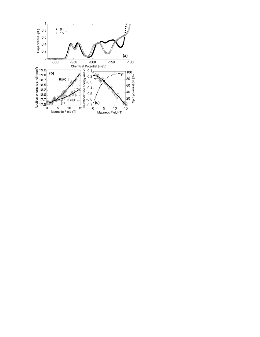
Figure 1: (a) Capacitance spectra taken at zero (solid circles) and 15 T (open squares) for $\mathbf{B}\parallel[001]$. The peaks associated to the s and p states can be easily identified, as well as the effect of the magnetic field on the orbital properties. The background corresponding to the geometrical capacitance has been removed. (b) Addition energy for n=2 (s-shell filling) as a function of the applied magnetic field for $\mathbf{B}\parallel[001]$ (open circles) and $\mathbf{B}\parallel[110]$ (open squares). The solid lines are fits using equation 5. (c) Helmholtz Free Energy $F_{1/2}$ (solid lines) and the experimental data, extracted from the $\mu_{1}$ dependence on the magnetic field, where we retained only the spin contribution; the orbital term $\hbar\Omega$ and the z confinement energy $E_{z}$ were subtracted. Spin polarization (dashed line) associated with the derivative of the measured addition energy plotted analytically as $tanh(g\beta B/2k_{B}T)$ using the inferred g factor and temperature.

Capacitance spectra at two different magnetic fields are shown in figure 1a. In order to analyze the data from an ensemble of quantum dots, we fit gaussian functions to each tunneling event. Solving the sum and difference between the position of the s-state gaussian peaks, we obtain $\hbar\omega_{0}=37.8\pm 0.2meV$, $E_{z}=280meV\pm 2meV$, $E_{C}(0)=17.2meV\pm 0.2meV$. The electrostatic interaction $E_{C}$ can be calculated from $\hbar\omega_{0}$ in the parabolic confinement assumption warburton , with an agreement better than 5-10% with the measured values of $E_{C}$.

In our analysis, we fit the peak difference using the equation 5 as showed in figure 1b, using the g-factor as the fitting parameter. The g factor for the s shell is found to be anisotropic prlthiago : $g_{[001]}=1.51\pm 0.05$ and $g_{[110]}=0.87\pm 0.05$. For $B\rightarrow 0$, $\Delta\mu\sim kT$, which can be verified in figure 1b.

The main feature in figure 1b is that the addition energy evolution with the magnetic field is not linear for fields below approximately 5 T. This is directly related with the lack of spin orientation for the loaded electrons due to thermal disorder acting to randomize the magnetic moments. In figure 1c we plot the Helmholtz free energy $F_{J}(B,T)=-kTln[2cosh(g\beta B/2kT)]$, extracted from the position $\mu_{1}$ of the first capacitance peak as a function of B. The polarization M is shown by the dashed line, calculated from the functional form of $F_{J}(B,T)$ and the fitting parameter g. We can identify 5 T as the field at which 80% of all spins are polarized with $\mathbf{B}||[001]$. For $\mathbf{B}$ parallel to the plane, this point is higher due to a smaller g-factor. The inferred polarization agrees with the empirical value utilized in an experiment of spin-selective optical absorption at 8 T 90 .

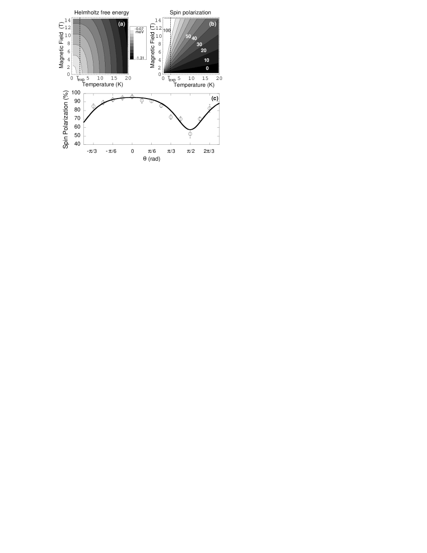
Figure 2: (a) Calculated Helmholtz Free Energy $F_{J}$ as a function of the magnetic field and temperature, evaluated from the measured values of g for the s shell for $\mathbf{B}||[001]$. (b) Associated spin polarization $\partial F_{J}/\partial B$. The temperature utilized during the experiments is represented by the dashed lines. (c) Angular dependence of the spin polarization for B=10T and T=2.7K. The experimental data is shown by empty circles.

Finally, we can infer from these results the polarization dependence on the temperature. Figure 2a shows that the Helmholtz free energy dependence on B and T. Above 15 K, the spin contribution to the addition energy is negligible. Figure 2b shows that for 5 K, field in excess of 15 T are required to fully polarize the spins. In figure 2c, the angular dependence of the polarization is shown. The degree of polarization varies between 90 and 50%, in agreement with a recent theoretical investigation hawrylak .

In summary, we were able to determine the degree of polarization of a system of non-interacting spins at finite temperatures and magnetic fields. The angular dependence reflects a spin polarization anisotropy due to the g-tensor characteristics, which should be taken into account in the interpretation of polarization experiments.

This work was supported by the MCT-CNPq and HP-Brazil. FGGH and TPMA would like to acknowledge FAPESP contracts 04/02814-6 and 04/01228-6 for financial support. We thank the IFGW-UNICAMP for the use of the high magnetic field facility.

References

- (1) J. A. Gupta, D. D. Awschalom, X. Peng, and A. P. Alivisatos, Phys. Rev. B 59, 10421 (R) (1999).
- (2) Y. Chye, M. E. White, E. Johnston-Halperin, B. D. Gerardot, D. D. Awschalom, and P. M. Petroff, Phys. Rev. B 66, 201301(R) (2002).
- (3) W. Löffler, M. Hetterich, C. Mauser, S. Li, T. Passow, and H. Kalt, Appl. Phys. Lett. 90, 232105 (2007).
- (4) C. H. Li, G. Kioseoglou, O. M. J. van ’t Erve, M. E. Ware, D. Gammon, R. M. Stroud, B. T. Jonker, R. Mallory, M. Yasar, and A. Petrou, Appl. Phys. Lett. 86, 132503 (2005).
- (5) L. Lombez, P. Renucci, P. F. Braun, H. Carrère, X. Marie, T. Amand, B. Urbaszek, J. L. Gauffier, P. Gallo, T. Camps, A. Arnoult, C. Fontaine, C. Deranlot, R. Mattana, H. Jaffr s, J.-M. George, and P. H. Binh, Appl. Phys. Lett. 90, 081111 (2007).
- (6) K. Gündoğdu, K. C. Hall, T. F. Boggess, D. G. Deppe and O. B. Shchekin, Appl. Phys. Lett. 84, 2793 (2007).
- (7) G. Itskos, E. Harbord, S. K. Clowes, E. Clarke, L. F. Cohen, R. Murray, P. Van Dorpe, and W. Van Roy, Appl. Phys. Lett. 88, 022113 (2006).
- (8) C.E. Pryor and M.E. Flatté, Phys. Rev. Lett. 91, 257901 (2003).
- (9) W. Sheng and P. Hawrylak, Phys. Rev. B 73, 125331 (2006).
- (10) L. M. K. Vandersypen, J. M. Elzerman, R. N. Schouten, L. H. Willems van Beveren, R. Hanson, and L. P. Kouwenhoven, Appl. Phys. Lett. 85, 4394 (2004).
- (11) G. Medeiros-Ribeiro, M. V. B. Pinheiro, V. L. Pimentel, and E. Marega, Appl. Phys. Lett. 80, 4229 (2002).
- (12) G. Medeiros-Ribeiro, E. Ribero, and H. Westfahl Jr., et. al, Appl. Phys. A 77, 725 (2003).
- (13) L. He, A. Zunger, Phys. Rev. B 73, 115324 (2005).
- (14) R.J. Warburton, C.S. Dürr, K. Karrai, J.P. Kotthaus, G. Medeiros-Ribeiro, and P.M. Petroff, Phys. Rev. Lett. 79, 5282 (1997).
- (15) R. J. Warburton, B. T. Miller, C. S. Durr, C. Bodefeld, K. Karrai, J. P. Kotthaus, G. Medeiros-Ribeiro, P. M. Petroff, and S. Huant, Phys. Rev. Lett. 58, 16221 (1998).
- (16) S. Raymond, S. Studenikin, A. Sachrajda, Z. Wasilewski, S.J. Cheng, W. Sheng, P. Hawrylak, A. Babinski, M. Potemski, G. Ortner, and M. Bayer, Phys. Rev. Lett. 92, 187402 (2004).
- (17) T.P. Mayer Alegre, F.G.G. Hernández, A. L. C. Pereira, and G. Medeiros-Ribeiro, Phys. Rev. Lett. 97, 236402 (2006).
- (18) , as shown in prlthiago .
- (19) Electron Paramagnetic Resonance of Transition Ions, A. Abragam (Clarendon Press, Oxford, 1970).
- (20) R. Hanson, L. P. Kouwenhoven, J. R. Petta, S. Tarucha, and L. M. K. Vandersypen, Rev. Mod. Phys. 79, 1217 (2007).
- (21) G. Medeiros-Ribeiro, F. G. Pikus, P. M. Petroff, and A. L. Efros, Phys. Rev. B 55, 1568 (1997).
- (22) A. Högele, M. Kroner, S. Seidl, K. Karrai, M. Atatüre, J. Dreiser, A. Imamoğlu, R. J. Warburton, A. Badolato, B. D. Gerardot, and P. M. Petroff, Appl. Phys. Lett. 86, 221905 (2005).