Stellar dynamics of blue compact galaxies

Abstract

Context. Luminous blue compact galaxies, common at $z\sim 1$ but now relatively rare, show disturbed kinematics in emission lines.

Aims. As part of a programme to understand their formation and evolution, we have investigated the stellar dynamics of a number of nearby objects in this class.

Methods. We obtained long-slit spectra with VLT/FORS2 in the spectral region covering the near-infrared calcium triplet. In this paper we focus on the well-known luminous blue compact galaxy ESO 338-IG04 (Tololo 1924–416). A previous investigation, using Fabry-Perot interferometry, showed that this galaxy has a chaotic H$\alpha$ velocity field, indicating that either the galaxy is not in dynamical equilibrium or that H$\alpha$ does not trace the gravitational potential due to feedback from star formation.

Results. Along the apparent major axis, the stellar and ionised gas velocities for the most part follow each other. The chaotic velocity field must therefore be a sign that the young stellar population in ESO 338-IG04 is not in dynamical equilibrium. The most likely explanation, which is also supported by its morphology, is that the galaxy has experienced a merger and that this has triggered the current starburst. Summarising the results of our programme so far, we note that emission-line velocity fields are not always reliable tracers of stellar motions, and go on to assess the implications for kinematic studies of similar galaxies at intermediate redshift.

1 Introduction

In the early universe, luminous, blue, compact galaxies (LBCGs) were much more common than they are now. Compact, emission-line-dominated galaxies with blue colours, small radii and disturbed morphologies (e.g. Koo et al. 1995; Guzman et al. 1996) may have accounted for nearly half of all star formation (Guzman et al. 1997) at redshifts between 0.4 and 1. Since then, the contribution from such galaxies has dropped by a factor of about ten (Werk et al. 2004; Guzman et al. 1997; Garland et al. 2007, and references therein).

LBCGs at all redshifts show both disturbed morphology and often also disturbed gas kinematics (Östlin et al. 1999, 2001; Gil de Paz et al. 1999; Pisano et al. 2001; Bershady et al. 2005; Puech et al. 2006). These have been interpreted as signs of a merger history (Östlin et al. 2001), and disturbed velocity fields are reproduced in models of merging galaxies (Jesseit et al. 2007; Kronberger et al. 2007). There is, however, no a priori reason to assume that the stars and the emitting gas in these galaxies share the same kinematics. Moreover, Östlin et al. (2001), studying the H$\alpha$ velocity fields of Östlin et al. (1999), found LBCGs in their sample with apparent dynamical mass deficiencies that could be attributed to non-equilibrium gas kinematics. Their results imply that this may be the rule rather than the exception for the subclass of very luminous blue compact galaxies. Such discrepancies could arise either because the gas is not in equilibrium with the gravitational potential of the galaxy, or because the gas motions are not solely in response to the gravitational potential. This second possibility, which could be due to feedback in the form of outflows, bubbles and superwinds, called for an investigation of the stellar kinematics of BCGs. Do the gas and stars in these galaxies move in concert or independently of one another?

This issue is important for assessing kinematic studies of star-forming galaxies at high and intermediate redshift, where velocity fields computed from emission lines may be the only observational way to probe of the gravitational potential. Kobulnicky & Gebhardt (2000) have compared slit spectra of a sample of 22 local late-type galaxies, among them the LBCG He 2-10, in emission lines ([O ii], Balmer lines and H i 21 cm) and Ca ii H and K. They concluded that stellar velocities and velocity dispersions generally agreed well with those of the ionised gas, and the agreement was particularly good for He 2-10. Moreover, Terlevich & Melnick (1981) have described a relation between velocity dispersion and H$\beta$ luminosity in extragalactic giant H ii regions, which has been used to estimate masses (e.g. Guzman et al. 1996; Östlin et al. 2001). Melnick et al. (1987) concluded that the relation is most likely determined by the virial motions of young stars.

To investigate the relationship between gas and stellar kinematics, we have collected kinematic data for a number of LBCGs. Our tactic has in each case been to trace the velocity field of the stars using the infrared triplet of Ca ii and compare with the velocity field seen in emission lines such as [S iii] $\lambda$9069 and the Paschen series of H i. The first results of this program were presented in Östlin et al. (2004, hereafter Paper I), where we used long-slit spectra to investigate the stellar and gas kinematics of ESO 400-G43. In Marquart et al. (2007) we used integral field spectroscopy to map the kinematics of He 2-10 in both emission lines and stellar absorption lines. In future we will present similar analyses for Haro 11 (ESO 350-IG38), ESO 480-IG12 and II Zw 40. In this paper we present new long-slit spectra of ESO 338-IG04, which has a disturbed velocity field in H$\alpha$ (Östlin et al. 2001). In the light of our results, we also take the opportunity to summarise what we currently know about the stellar and gas motions in LBCGs.

2 Observations and data reduction

We have carried out long-slit spectroscopy with FORS2 on the 8-m telescope UT2/Kueyen at the VLT. ESO 338-IG04 was observed between 2000 July 03 and 2000 August 03 using the Tektronix 2048$\times$2048-pixel CCD.

Table 1: Log of observations

Date	Object	Seeing	Slit	Total integration
(UT)		(arcsec)	PA (∘)	time (s)
2000 07 03	ESO 338-IG04	0.7-1.2	90∘	8100
2000 07 04	ESO 338-IG04	0.9-1.2	160∘	1800
2000 07 29	ESO 338-IG04	0.6-0.8	90∘	4200
2000 08 02	ESO 338-IG04	1.0-1.4	90∘	1200
2000 08 03	ESO 338-IG04	0.4-0.7	90∘	3600
2000 08 03	ESO 338-IG04	0.4	160∘	1800

Notes: Wavelength coverage was 7850-9230 Å. The spectral resolution, measured from the width of unresolved extracted sky emission lines, was 67$\pm$3 km s^-1

2.1 ESO 338-IG04

Figure 1: Positions of slits PA 90^∘-270^∘ and 160^∘-340^∘ superimposed on an HST narrow-band H$\alpha$ (F656N) image of ESO 338-IG04 taken from Hayes (2007). North is up and east to the left. The positions of prominent super star clusters are marked, numbered according to Östlin et al. (1998). All the clusters belong to their inner sample, except 21, 25 and 47, which belong to the outer sample. The bright object to the lower right is a foreground star. The field of view here is 22″ by 18″, corresponding to 3.9 kpc by 3.25 kpc at the distance of ESO 338-IG04 (37.5 Mpc; Östlin et al. 1998).

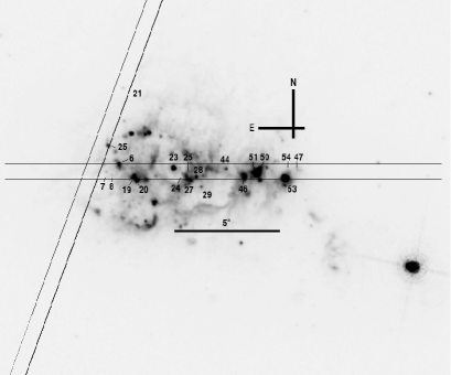
For our long-slit spectroscopy, we used a slit of width 0.7″ at two different positions for ESO 338-IG04. Figure 1 shows the slit positions relative to the the star clusters and the nebular emission in the galaxy. One slit was aligned along the major axis of the galaxy, at position angle 90^∘-270^∘. At this position we integrated for a total of 18000 s, divided into 1200- and 900-second exposures. The other slit was chosen to investigate the steepest velocity gradient seen in H$\alpha$ data for the galaxy (Östlin et al. 1999, see also Figure 6), at position angle 160^∘-340^∘ and centred 3.7″ east of the central concentration (cluster #23 in the inner sample of Östlin, Bergvall, & Rönnback 1998). At this position, however, we obtained only 4$\times$900-s integrations due to time constraints. We used the G1028z grism, which gave a spectral resolution of about 4500 (67$\pm$3 km s^-1, as measured from unresolved sky lines) near the Ca ii triplet.

We followed a standard reduction procedure using iraf. We bias-subtracted and flat-fielded the science frames in the usual way, using dome flats to create a mean flat field frame. Then we removed by hand cosmic ray hits that lay close to the lines we are most interested in, since we found that not all cosmic rays were properly removed by median-filtering the final registered spectra. Wavelength calibration was carried out using the OH sky lines, with wavelengths from Osterbrock & Martel (1992) and Osterbrock et al. (1996).

The resulting long-slit spectra were combined, shifting first so that the galaxy centroid along the slit was the same in each case. While the spectra were taken under a variety of conditions, and some observations were affected by poor atmospheric transparency, the seeing was generally good (Table 1). We tested different averaging methods and excluding the poorer data, and found that the best signal-to-noise ratio in the final result was obtained by median-filtering all the spectra and weighting according to detected counts in the continuum at 8610-8700 Å. For this we used the task scombine in iraf. The resulting wavelength-calibrated, two-dimensional spectrum was used for the subsequent analysis.

2.2 Extraction and flux-calibration

From our final spectra for each slit, one-dimensional extractions were made at intervals in the spatial direction (3 detector rows, or 0.75″). The sky background was subtracted from the ESO 338-IG04 spectra at this stage, linearly interpolating between regions free of galaxy emission on each side of the galaxy. For this we used patches $\sim$1 arcmin wide displaced by 50″ from the centre.. The extracted spectra were in turn flux-calibrated by comparison with spectra taken of the standard stars LTT 7379 and LTT 7987 using the same set-up.

While we have not corrected our spectra for telluric absorption, the region containing the Ca ii triplet is relatively free from such features. In our analysis we have also avoided the region longward of 9000 Å where the H₂O bands are strong (see for example Figure 16 in Matheson et al. 2000). The emission lines Pa 11, Pa 10 and [S iii] $\lambda$9069 do lie in this region, but our iterative procedure for Paschen-subtraction is unlikely to be affected by telluric features.

2.3 Subtracting emission lines

Table 2: Template stars for cross-correlation analysis.

Star	Type/class
HD 164349	K0 ii-iii
HD 172365	F8 ib-ii
HD 174947	K1 iB
HD 174974	K1 ii
HD 175751	K2 iii
HD 179323	K1 i

Note: Spectral types and luminosity classes are taken from the VizieR database (Ochsenbein et al. 2000).

Figure 2: Three examples of Paschen-line subtraction from the spectrum of ESO 338-IG04 around the calcium triplet, for extractions with different signal to noise ratio and different quality of subtraction, using the less affected blue wing of each line as a guide. These subtractions, for the slit at PA 90–270°, were classed as high (top; position $-$2″.7), medium (middle; +1″) and low (bottom; $-$1″.2). Positions are relative to the point where the two slits cross; see section 3. The subtracted spectrum is plotted over the original spectrum (grey). Vertical dashed lines mark the approximate expected position of the centres of the three calcium triplet lines.

Our aim was to compare the extracted galaxy spectra around the Ca ii triplet with the spectra of template stars of different types (Table 2). The spectra are however dominated by narrow emission lines, primarily the H i Paschen series. To remove these lines and achieve a clean spectrum of the galaxy’s stars alone, we model and subtract the Paschen series lines. We have described our Paschen-subtraction technique in Paper I. For ESO 338-IG04, where the emission lines are stronger relative to the stellar absorption lines, we refined the Paschen-subtraction procedure.

We measured the fluxes of the strongest Paschen lines from our spectra, excluding those which overlap with the Ca ii triplet, and compared with the predicted strengths for Case B recombination at a temperature of 10⁴ K and density 100 cm^-3 given by Osterbrock (1989). Within the likely errors of our measurements, the lines follow the predicted values. This is consistent with the low extinction values used for these galaxies by Östlin et al. ($E_{B-V}<0.1$;  1998), and we have therefore made no extinction correction to our data or models. The Paschen decrement does not vary significantly across our slits, indicating no significant variation in extinction.

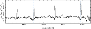
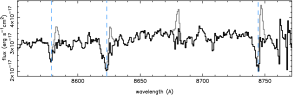
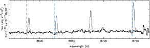
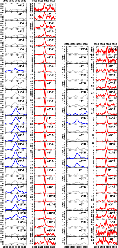
An initial, first-guess model profile for each line was constructed by fitting a number of Gaussians to the high signal-to-noise [S iii] $\lambda 9069$ line. This model profile was then shifted to match the measured redshifts of the strongest Paschen lines in the spectrum, creating a model spectrum of the Paschen series from Pa 9 to Pa 20. We scaled this spectrum to match the strongest clean Paschen lines (Pa 10, Pa 11, Pa 12 and Pa 14) and finally subtracted it from the observed spectrum (Figure 2). Thereafter we adjusted the width, redshift and strength of the lines, iterating in order to produce plausible subtractions. In practice this meant minimising the subtraction residuals around the clean Paschen lines and ensuring that the red wing of each corrected Ca ii absorption feature was plausibly consistent with its less contaminated blue wing.

We judged the reliability of each subtraction qualitatively, dividing the subtractions into three classes of high, medium and low quality. In particular, where the risk of over- or undersubtraction was large and the emission lines were particularly strong, the low-quality classification is chosen. In our subsequent analysis, we have only included those with high or medium quality. Figure 2 shows examples of each level.

Finally, we removed sky subtraction residuals and the remaining strong emission line O i $\lambda$8446 by linearly interpolating across it. Figure 2 shows examples of prepared spectra.

Figure 3: Cross-correlation functions with respect to HD 164349 (blue/darker and grey/lighter profiles; first and third panels) and [S iii] profiles (in red; second and fourth panels) for ESO 338-IG04. The left two boxes are for slit PA 90^∘-270^∘ and those on the right are for PA 160^∘-340^∘. Positions in arcsec relative to the crossing point of the two slits are marked next to each profile. CCFs are plotted in grey where the Paschen subtraction quality is low, or where the peak of the CCF is less than 0.25. Units in each plot are (abscissae) velocity in km s^-1 and (ordinates) CCF value or flux in units of $10^{-17}$ erg s^-1 cm^-2.

2.4 Deriving the stellar kinematics

To ensure robust measurements of the stellar velocity field, we have used two independent methods, cross-correlation with template stars (section 2.4.1) and penalized pixel-fitting (pPXF; section 2.4.2).

2.4.1 Method 1: Cross-correlation with template stars

We used the iraf task fxcor to cross-correlate the prepared spectra with our six template stars on the region containing the Ca ii triplet. For this we used only the region 8377-8948 Å, i.e. only Paschen-subtracted part of the spectrum, as far red as the start of the stronger telluric absorption bands at longer wavelengths. To ensure that strong signals from pixel-to-pixel noise and low-frequency undulations in the spectra did not affect measurements of the cross-correlation function (CCF) peak, we experimented with a ramp filter defined in fxcor. In this we follow Tonry & Davis (1979) and Wegner et al. (1999). We found that the best correction for pixel-to-pixel noise resulted from a ramp rising from zero to unity at wavenumber 15 (wavenumbers here correspond to power at different numbers of spectral pixels in the prepared spectrum). For a good match between the low-frequency behaviour of the template and galaxy spectra, we found we needed the ramp filter to fall to zero between wavenumbers 1000 and 1100.

The resulting CCFs are shown in Figure 3. We measured the width and velocity of each peak by fitting a Gaussian on the region above 60 percent of the peak height.

For measuring the heliocentric velocity, we required accurate radial velocities for the template stars (Table 2). We used catalogue radial velocities from the VizieR database (Ochsenbein, Bauer, & Marcout 2000) and for consistency cross-correlated between pairs of template stars to determine better radial velocities for some of them. To do this we adjusted the least precisely determined velocities in turn, in order to minimise the sum of the squares of the differences between the expected and measured velocity difference in each pair.

For errors in heliocentric velocities, we have used the errors calculated by fxcor.

To be able to measure the velocity dispersion $\sigma$, we empirically determined the relationship between the width of the peak of the cross-correlation function and the value of $\sigma$. To do this we broadened the template star spectra with Gaussians of various widths (i.e. known $\sigma$), and compared the resulting velocity width $v_{\rm FWHM}$ of the cross-correlation peak with the value of $\sigma$ (Nelson & Whittle 1995; Ho & Filippenko 1996a, b). To avoid systematic errors in this process, we used the same procedure here described for similar measurements in Östlin et al. (2007), adding noise to match the value of the CCF peak. This ensures that the relation between $v_{\rm FWHM}$ and $\sigma$ is not affected by mismatches in data quality.

The velocity curve determined from cross-correlations is independent of the choice of template star. The mean values between +3.2″ and +7.8″, for example, all agree to within the errors with a velocity of 2833.5 km s^-1. The derived velocity dispersions, on the other hand, are much larger for the F8 ib-ii template star HD 172365 (mean value $\sigma=114\pm 9$ km s^-1, compared to a mean of $64\pm 4$ km s^-1 for the others). This star has broader CaT lines than our other template stars, and the implication here is that our technique for calibrating velocity dispersions breaks down when line widths in the object and template spectra are comparable. We do not include HD 172365 in our subsequent analysis.

For our velocity dispersion measurements, we found that the dominant source of uncertainty, particularly where the signal-to-noise ratio was low, was the identification of the CCF peak and the Gaussian fit to it. To quantify the errors introduced in this way to each measurement of $v_{\rm FWHM}$, we followed the same procedure as Östlin et al. (2007), investigating the range of plausible Gaussian fits to the CCF peak. We then used the standard error in these measurements as an estimate of the error. In contrast to Östlin et al. (2007), we found that the errors found in this way are larger than those introduced by the scatter in the $v_{\rm FWHM}-\sigma$ calibration relation. The errors were then propagated through the calibration procedure described above. This method is not rigorous but gives, we believe, acceptable estimates of the error in $\sigma$.

For some positions with poor signal-to-noise in the stellar spectrum, the cross-correlation function peaks at values too low to provide reliable estimates of either the velocity or the velocity dispersion. We have therefore defined a cut-off for acceptable cross-correlations at CCF value 0.25.

2.4.2 Method 2: Penalised pixel-fitting

We have also derived the stellar kinematics using the penalised pixel fitting (pPXF) method developed by Cappellari & Emsellem (2004). In this case we fitted the lines in real pixel space, since it is easier to mask the spectra to remove bad pixels or regions contaminated by emission lines. We made use of a large library of high resolution observed and model spectra (Cenarro et al. 2001a, b). We created linear combinations of these template spectra to match with the galaxy spectrum and fit the stellar kinematics. The parameters ($V$, $\sigma$, $h_{3}$, $h_{4}$) were fitted simultaneously, with an adjustable penalty term added to the $\chi^{2}$ to bias the solution towards a Gaussian shape when the higher order terms (skewness $h_{3}$ and kurtosis $h_{4}$) are unconstrained.

To make the pPXF routine deliver the best template spectrum quickly, we picked out a restricted set of 17 stellar spectra from the Cenarro library. These spectra were carefully chosen to cover a wide range of stellar types: dwarfs, giants, and supergiants, spectral classes O9 v ($T_{\rm eff}$=36 300 K) to M6 v ($T_{\rm eff}$=3720 K), with metallicities ranging from [Fe/H]=$-$2.25 to 0.13 solar. The best matching combined spectrum can thus represent regions with distinctly different stellar populations. However, since there is more than one combination of stellar mixes that can reproduce the absorption features in a galaxy spectrum, the weights assigned to individual stellar spectra could not be used to carry out a population analysis for our galaxies.

We investigated the robustness of the kinematic parameters delivered by pPXF by changing the input stellar library, masking out the red wings of the CaT lines which are where imperfections in the Paschen-line subtraction could change the derived stellar kinematic parameters, and finally by applying a higher weight to the stronger absorption features. We found that in all these cases, we were still able to derive similar velocities and velocity dispersions.

To estimate errors for the pPXF kinematic parameters, we applied the bootstrap Monte Carlo method (Chapter 6 of Press et al. 1992). We ran 300 simulations, varying the input stellar library, both by adding and subtracting template stars and by using one star at a time. We found that the derived kinematical parameters for the full library of 17 template stars with parameters derived for a subset of these or individual stars, all fall within $\pm 30$ km s^-1 of the adopted values. This therefore gives an upper limit for the errors. Additionally, we found that for the noisier spectra, the pPXF method can produce a spurious fit to the spectra with weak narrow Ca ii lines which clearly cannot be justified by the data. We have flagged these points and do not include them in our analysis.

2.5 Systematic errors

Our results from cross-correlation and pPXF agree well, and deliver comparable stellar velocities and velocity dispersions. This indicates that the kinematics in ESO 338-IG04 can be derived in a robust way from our prepared spectra. Both cross-correlation and pPXF deliver comparable stellar velocities, and the choice of stellar template is not important as long as the star is a late-type giant or supergiant.

A remaining source of systematic error is our Paschen-subtraction procedure. To quantify this, we scaled the flux of each model spectrum to produce plausible over- and under-subtractions. We then redetermined the kinematics using pPXF and examined both the quality of the fit ($\chi^{2}$) and the resulting changes in the derived velocity and velocity dispersion. For all our spectra, we found the minimum of $\chi^{2}$ to fall within 10% of the adopted strength of the Paschen subtraction. This corresponds to systematic errors in both velocity and velocity dispersion of at most 10 km s^-1. Moreover, we see no systematic trend towards over- or under-subtraction, giving us confidence that our method provides a reliable correction for H i emission at each position.

2.6 Deriving the gas kinematics

Emission-line velocities, widths and fluxes were measured from Gaussian fits to the lines carried out interactively using the IRAF task splot. The velocity dispersion in each emission line was calculated by subtracting the instrumental width in quadrature from the measured line width. Errors were estimated from the scatter in the measured values for lines of different measured flux. For the Paschen lines we calculated weighted means for the velocities and widths using all the available lines at each position.

3 Results

In the following we quote positions in arcsec along our slits relative to the point where the two slits cross (Figure 1). Positive values for the two slits are towards the west (PA 270°) and north (PA 340°), respectively.

Figures 4 and 5 show the measured velocities and velocity dispersions plotted against position along the two slits in ESO 338-IG04. The plots show results from both the cross-correlation and pPXF methods and also the spatial variation of the continuum level near the CaT lines (for the stars) and emission line flux (for the gas).

Figure 4: Variation along slit PA 90^∘-270^∘ of (from top to bottom) continuum/line flux, velocity dispersion $\sigma$ and heliocentric velocity, for the gas (left) and stars (right) in ESO 338-IG04. Zero on the abscissa is defined as the point where our two slits cross, 4″ east of cluster #23. The left panel shows the emission lines [S iii] $\lambda$9069 (red open circles), H i Paschen lines (weighted means of all measured lines; blue filled circles), and O i $\lambda$8446 (green squares). The flux scales show (left) the normalised strengths of the emission lines and (right) the [S iii] line flux compared to the mean continuum value around the calcium triplet. The dotted vertical lines mark the positions along the slit of (from left to right) clusters 6, 19, 23, 44 and 53 from the inner sample of Östlin et al. (1998) (see also Figure 1). The right panel shows results of cross-correlation with the K0 bright giant HD 164349 (blue squares) and pPXF results (magenta open circles). Cross-correlation measurements of velocity dispersion and heliocentric velocity are only shown where the CCF peak is greater than 0.25. CCF and pPXF results are not shown where the Paschen-subtraction quality was deemed to be low (see Figure 2). The thick dashed line in the right panel repeats the [S iii] results from the left panel for comparison. At the distance of ESO 338-IG04, 10″ corresponds to 1.8 kpc.

Figure 5: Same as Figure 4, but for ESO 338-IG04 at PA 160^∘-340^∘. The dotted vertical lines in this case mark the positions along the slit of clusters 25 (left) and 21 from the outer sample of Östlin et al. (1998) (see Figure 1).

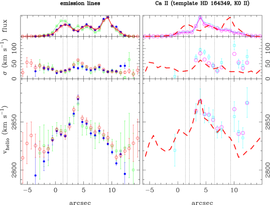
Along the slit at PA 90^∘-270^∘, the emission lines show close to identical velocity curves, and show the same features as the H$\alpha$ observations of (Östlin et al. 1999, Figure 6). The velocity field has a span of about 60 km s^-1 with local minima at $-$2″ and +11″, and a barely resolved (1.5″-wide) local maximum with amplitude $\sim$30 km s^-1 at the position of cluster #23 (+4″).

Although the stellar velocity field is much less well-determined than that of the gas, some trends are nevertheless evident. Just as for the emission lines, no strong velocity gradient is detected. Indeed, the data are marginally consistent with a flat rotation curve with velocity 2860 km s^-1. A more interesting null hypothesis, however, is that the stars show the same velocity field as the gas. Between +3″and +8″the agreement is clear from Figure 6. Between +10″ and +13″, however, the stars and gas differ at the 3-$\sigma$ level: the mean stellar velocity is 2846$\pm$8 km s^-1 (taking the mean of all the template stars), while the velocity in [S iii] $\lambda$9069 is 2822$\pm$1 km s^-1.

Over the 6 arcseconds ($\sim$1 kpc) west of cluster #23 (position +4″), a shallow gradient of 40 km s^-1 suggests a solid body rotation curve centred at $\sim$+6″. Similarly, while the two-dimensional H$\alpha$ velocity field (Figure 6 and Östlin et al. 1999) is far from ordered, a kiloparsec-scale region just west of the centre is nevertheless consistent with solid body rotation and with the data we present here. If interpreted as solid body rotation with the same inclination (55°) indicated by the axis ratio of the outer isophotes, a rotational mass of the order of $3\times 10^{7}$ M_⊙ is implied. This is significantly smaller than the stellar mass of the central region, which is at least $2\times 10^{8}$ M_⊙ (Östlin et al. 2001). The velocity dispersion of stars and gas in this region is on the other hand 50 km s^-1 or more, which indicates a dynamical mass in excess of $10^{9}$ M_⊙ if we can assume dynamical equilibrium.

The slit passes through a number of the young star clusters identified by Östlin et al. (1998) (Figure 1). Of these, only at the very massive cluster #23 (at +4″), where the gas rotation curves take a narrow excursion to the red, do we see any possible effect on the stellar velocities. This position coincides with the maximum of the galaxy’s continuum flux distribution and although cluster #23 accounts for up to half the continuum flux there, a number of other clusters contribute to the signal at this position in the slit. Here we also observe a gap in the [S iii] and Paschen-line emission, consistent with the bubble-like distribution of emission (Östlin et al. 2007) seen in the HST H$\alpha$ image.

To investigate the source of the peak in the velocity curve, we co-added the six two-dimensional spectra with the best seeing and examined the structure around the [S iii] $\lambda 9069$ line. Inside the gap at the position of #23 there is a distinct, fainter emission component with velocity about 2900 km s^-1, about 50 km s^-1 redder than the surrounding gas. Emission components at $-$45 and +20 km s^-1 relative to the stellar velocity of #23 were observed by Östlin et al. (2007) in H$\alpha$ and [O iii] in their slit passing through #23 at PA 43^∘. Our extracted [S iii] profiles show signs of these components (Figure 3). At +4″, the profile is distinctly flat-topped. Inspection shows that the neighbouring profiles are asymmetric with shallower red wings, giving the impression that a redshifted component reaches its maximum at +4″, and is weaker on either side. The velocity we measure in Ca ii at the position of #23 is identical within the errors to the cluster’s velocity as measured by Östlin et al. (2007) (2860$\pm$4 km s^-1), so it seems likely that we are seeing the same expanding bubble around #23 which Östlin et al. (2007) identified.

The velocity dispersion in the emission lines varies little along the slit. It peaks at around 50 km s^-1 at +4″ and again at +8″. These positions correspond to minima between the three main concentrations of line emission along the slit. The stellar velocity dispersions are larger than those of the gas: about 70$\pm$20 km s^-1 compared to 40$\pm$10 km s^-1 for the ionised gas at positions where both are measured. We caution, however, that since the measured velocity dispersions are comparable to the instrumental resolution (about 60 km s^-1), the errors in the velocity dispersion measurements may well be underestimated.

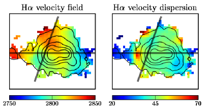
In Figure 6 we reproduce the spatially resolved kinematics in the H$\alpha$ line by Östlin et al. (1999). We find good agreement with our data presented here. The decline in velocity towards both sides of the center at PA 90°-270° is well-reproduced, as is the velocity difference along PA 160°-340°. Due to the lower spatial resolution of the H$\alpha$ data, the feature at cluster #23 discussed above cannot be seen in Fig. 6. On the other hand, our slit spectra do not reach deep enough in the Paschen lines to cover the tail toward the east where the velocity rises again, or the peak in the velocity dispersion ($\sigma\approx 60\>\mbox{\rm km\leavevmode\nobreak\ s\mbox{${}^{-1}$}}$) at 4″.5 east of where our two slits cross. We do however see a local maximum in velocity dispersion in [S iii] at position $-$5″ (Figure 4).

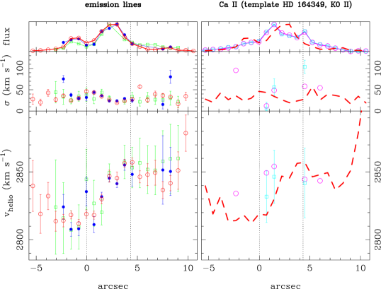
For the slit at PA 160^∘-340^∘ (Figure 5), the quality of the data is much poorer. In the emission lines, we confirm the velocity gradient between +1″ and +4″ noted by Östlin et al. (1999). Östlin et al. (2001) argued that this gradient is unlikely to be due to rotation, and is better explained by an outflow or a distinct dynamical component. The velocity curve is symmetric about position +2″, and flat beyond 0″ on one side and +4″ on the other, with a spread in velocity of 40 km s^-1. The velocity dispersion in the gas is constant at $\sim$30 km s^-1 across the slit. The calcium triplet lines are detected at at most two positions, corresponding to the eastern end of the galaxy’s central concentration at +1″, and the vicinity of cluster #25 (from the outer sample of Östlin et al. 1998). The gas and stars show no differences at either of these positions, though the stellar velocity dispersion at cluster #25 is higher than that for the gas.

We have also applied our current improved analysis methods to the ESO 400-G43 spectra presented in (Paper I). We find no significant changes in either the results or conclusions of Paper I.

4 Discussion

Figure 6: Velocity field (left) and velocity dispersion (right) of ESO 338-IG04 from Fabry-Perot measurements of H$\alpha$, as measured by Östlin et al. (1999). North is up and east to the left. The colour scales in km s^-1 are indicated below each panel. The black contours correspond to the H$\alpha$ flux in arbitrary logarithmic units. Overlaid in grey are the positions of our slits (cf. Figure 1). Each frame is 36.4″ wide, and one pixel corresponds to 0.91″ on the sky.

4.1 The dynamical history of ESO 338-IG04

Earlier studies have suggested mergers and interactions as the triggering mechanism of starbursts in luminous BCGs like ESO 338-IG04 (Östlin et al. 2001; Bergvall & Östlin 2002). Neutral hydrogen mapping of ESO 338-IG04 and its companion ESO 338-IG04 B (Cannon et al. 2004) showed evidence of a $\sim 2\times 10^{9}$-M_⊙ tidal tail stretching from just above the companion ESO 338-IG04 B to ESO 338-IG04 and beyond, indicating a strong interaction in the recent past. However, interaction with the companion is unlikely to have caused the present burst of star formation which was initiated about 40 Myr ago (Östlin et al. 2003). With a projected distance between the two galaxies of 70 kpc, such timing requires an extreme collision velocity of at least 1500 km s^-1. Moreover, the radial velocity difference of the two galaxies is only a few $\times$10 km s^-1, and the companion is dynamically well-behaved, both in H$\alpha$ (Östlin et al. 2001) and in H i 21 cm (Cannon et al. 2004). It is therefore more likely that the current burst is unrelated to ESO 338-IG04 B. For typical velocities of galaxy pairs and triples, of the order of 100 km s^-1, the last close passage of the two galaxies would have occurred on the order of 1 Gyr ago. Interestingly, this corresponds to a peak in the age distribution of the star clusters in ESO 338-IG04 (Östlin et al. 2003).

Based its morphology and its disturbed H$\alpha$ velocity field, Östlin et al. (2001) suggested a merger as the cause of the starburst in ESO 338-IG04. However, in addition to gravity, the interstellar medium in galaxies can also be affected by feedback from stellar winds and supernova explosions. For this reason, a chaotic H$\alpha$ velocity field alone is not necessarily proof of a merger. An independent measurement of the stellar and gas kinematics is required to separate the effects of gravity and feedback.

In ESO 338-IG04, we see that the velocity fields of the ionised gas and the young stellar population tend to follow each other. This demonstrates that this galaxy’s chaotic H$\alpha$ velocity field cannot be explained solely by feedback in the form of expanding bubbles and superwinds. Such processes certainly affect the velocity field, as witnessed by the bubbles along slit PA 160^∘-340^∘ and around cluster #23 (see above and Östlin et al. 2007). But the velocity curve traced in Ca ii is dynamically just as surprising as that of the gas.

Can we be sure that the Ca ii triplet is a reliable tracer of the stellar motions in the galaxy? The triplet lines become observable as soon as a stellar population is old enough to produce red giants and supergiants, i.e. after about 5 Myr, and by virtue of the strong starburst in ESO 338-IG04 the Ca ii triplet absorption is likely dominated by young supergiants. This is evident in our data, as we see strong Ca ii lines even where young super star clusters (SSCs) dominate. There is of course the possibility that the young population dominates the observed Ca ii velocity field, while the old stellar population is still kinematically well-behaved. This would require that the young stars were formed when an external gas cloud fell into the gravitational potential of the galaxy but did not have enough mass to significantly distort it. While we cannot be sure that this did not happen, it seems to us more likely that the Ca ii lines do indeed trace the major part of the stellar motions. In such a case, neither the stars nor the ionised gas are in dynamical equilibrium.

An additional clue to ESO 338-IG04’s history comes from the tail-like structure to the east of the starburst, observed in both H$\alpha$ (Östlin et al. 1999) and in optical and near-IR broadband filters (Bergvall & Östlin 2002). It has significantly bluer colours than the rest of the galaxy outside the starburst region. Moreover, it contains young star clusters (Östlin et al. 2003) and clearly cannot solely be due to gas emission. It is also coincident with a local maximum in the H i column density map (Cannon et al. 2004). Östlin et al. (2001) attributed this tail to a young, off-centre stellar population with, again, peculiar kinematics.

Taken together, all these observations leave only one plausible explanation for the origin of ESO 338-IG04’s starburst, morphology, globally peculiar H$\alpha$, H i and now its stellar kinematics. It must be the result of a recent merger, either with a dwarf galaxy or a massive neutral gas cloud. While we still do not know whether the stars are as disrupted as the gas on larger scales, a merger is still required to explain the disturbed central kinematics.

Whether ESO 338-IG04’s merger was with another galaxy or with a gas cloud is not a question we can answer given the current observations. What triggers a starburst is the supply of gas to the central regions (cf. Combes 2005), and this could be provided either by an infalling dwarf galaxy or massive cloud of gas. Indeed, large amounts of neutral gas are still present close to the galaxy: in addition to the tidal tail, the H i data of Cannon et al. (2004) also indicate an asymmetric distribution of neutral gas close to ESO 338-IG04, most concentrated on its west side. Moreover, the galaxy shows no evidence of a single nucleus, still less a double one, as might be expected after a merger.

In either case, if its lack of rotational support on small scales is also applicable at large galactocentric radii, ESO 338-IG04 may well be in the process of evolving into an early-type galaxy. Alternatively, the lack of central rotational support for the gas and stars in the starburst could be interpreted as the formation of a spherical or triaxial system, or a bulge (Hammer et al. 2005).

ESO 338-IG04 shows a discrepancy between its estimated stellar (photometric) mass and the dynamical mass inferred from the H$\alpha$ rotation curve (Östlin et al. 2001). Whereas a high dynamical mass is usually interpreted as evidence for dark matter, here the galaxy is not rotating fast enough to support its stellar mass. ESO 400-G43 (Paper I) is similar in this respect. In the case of ESO 338-IG04, Östlin et al. (2001) failed to derive a rotation curve where the receding and approaching sides agreed. The two-dimensional velocity field is clearly very irregular and suggests that the system is not in dynamical equilibrium (cf. Figure 6).

4.2 Stellar and ionised gas kinematics in blue compact galaxies

Adding our results to those of Paper I and Marquart et al. (2007) for He 2-10, we have now studied the stellar kinematics of three blue compact galaxies (BCGs) with disturbed velocity fields. Here we assess what the interim results of our programme have to say about BCGs as a class, both locally and at higher redshift.

We have now seen two cases where the gas and stars are clearly decoupled (He 2-10 and ESO 400-G43) and one where they for the most part follow one another (ESO 338-IG04). In ESO 338-IG04, moreover, we see evidence that the coupling between gas and stars can vary depending on position in the galaxy.

Our data has allowed us to identify three physical mechanisms that contribute to the dynamics of these galaxies.

Gas-star decoupling: The stellar and gaseous velocity fields differ from each other, due either to outflows triggered by supernova winds, or to infall in a merging process. We see this in both ESO 400-G43 (Paper I) and He 2-10 (Marquart et al. 2007).

Large-scale gravitational disturbances: The stellar velocity field is comparable to that of the ionised gas, and neither the stars nor the gas may trace the potential. This situation can indicate real dynamical disturbances of the type expected in mergers, and is what we observe in the central region of ESO 338-IG04.

Velocity dispersion provides support: Stellar velocity dispersions in late-type galaxies are usually small, but in galaxies which apparently lack rotational support, the velocity dispersion must contribute to the gravitational support (e.g. Côté, Carignan, & Freeman 2000). This could explain at least the low rotational velocities in He 2-10 and ESO 338-IG04, if not the shapes of their rotation curves, and is consistent with the observed emission-line widths and stellar velocity dispersions (Östlin et al. 2001). Elliptical-like galaxies could, it seems, be presently forming in these galaxies as a result of earlier mergers.

What are the implications for studies of similar galaxies at intermediate redshift (e.g. Bershady et al. 2005; Puech et al. 2006) Observations of local late-type galaxies (Kobulnicky & Gebhardt 2000) and ultraluminous infrared galaxies (Colina et al. 2005) have shown that stellar and emission-line velocity amplitudes and velocity dispersions are comparable. Our BCG measurements show that the stellar velocity dispersion is higher than that of the gas in ESO 338-IG04, and in He 2-10 the stellar velocity dispersion was lower than that of the gas in the centre of the galaxy (Marquart et al. 2007). So far, it seems that emission-line velocity fields in BCGs are not reliable tracers of the underlying stellar velocities. An extended study of the combined stellar and gas kinematics of a larger number local BCGs and other analogues of the compact narrow emission line galaxies at intermediate redshift is therefore required.

5 Conclusions

We have investigated the stellar velocity fields of the blue compact galaxy ESO 338-IG04, using the infrared Ca ii triplet. Using both cross-correlation with template stars and penalised pixel-fitting to determine velocities and velocity dispersions, we show that stars and gas can follow one another in these galaxies, but do not always do so.

Our new results exclude the possibility that the chaotic kinematics seen in the H$\alpha$ gas in the centre is simply the result of feedback and outflows, although such are probably present as well. We conclude that the centre of the galaxy is not rotationally supported, and that the current starburst was most likely triggered by a merger, either with a dwarf galaxy or a massive gas cloud.