Faltung Formulation of Hadron Halo Event Cascade at Mt. Chacaltaya

Abstract

It is shown that the fundamental standard hadron cascade diffusion equation in the Mellin transform space is not rigorously correct because of the inconsistent double energy integral evaluation which generates the function $<\eta^{s}>$ with its associated parametizations. To ensure an exact basic working equation, the Faltung integral representation is introduced which has the elasticity distribution function $u(\eta)$ as the only fundamental input function and $<\eta^{s}>$ is just the Mellin transform of $u(\eta)$. This Faltung representation eliminates standard phenomenological parameters which serve only to mislead the physics of cascade. The exact flux transform equation is solved by the method of characteristics, and the hadron flux in real space is obtained by the inverse transform in terms of the simple and essential residues. Since the essential residues are given by the singularities in the elasticity distribution and particle production transforms that appear in the exponentials, these functions should not be parametized arbitrarily to avoid introducing non-physical essential residues. This Faltung formulation is applied to the charged hadron integrated energy spectra of halo events detected at Mt. Chacaltaya by the Brazil-Japan Collaboration, where the incoming flux at the atmospheric boundary is a single energetic nucleon.

I Introduction

The Brazil-Japan Collaboration detected many cosmic-ray events in the energy range $(10^{13}-10^{17})\,eV$ with emulsion chamber exposed at Mt. Chacaltaya. About twenty events were observed in the visible energy region $E~{}\geq~{}1000\,TeV$. Approximately, half of them  lattes ; amato ; chinellato ; yamashita were associated with a uniformly darkened wide area on X-ray films. The central part of this area was called ”halo”, and so these events were called ”halo events”. Similar events were also observed in experiments at Pamir pamir ,Fuji akashi , and Kanbala ren . Recently, a new experiment aoki , using a hadron calorimeter associated with emulsion chambers at Mt. Chacaltaya, reported this kind of events as well. Thus, the appearance of a strong concentration of energy and particles as a halo seemed to be a common feature in this energy region. After the 1980s, these super-families were also compared with simulations using different primary compositions and models for high-energy nuclear interactions capedevielle ; kalmikov ; werner . Nevertheless, these simulations could not describe fully all the events with the same inputs on primary composition and nuclear collision models. Due to their large hadronic number and energy, some authors amato2 suggested that these events could be explained as centauro-like ones.

Recently, we have developed an analytic method tsui that allows us to calculate the hadronic and electromagnetic components of cosmic rays in the Earth’s atmosphere, and generalizes earlier works arata ; boyadzhyan ; bellandi86 ; ohsawa by including the energy dependence of the mean-free path effect. An important issue in the high energy region concerns the behavior of the inelasticity, which is defined as the fraction of energy given up by the leading hadron in a collision induced by an incident hadron on a target nucleon or nucleus. This parameter has been exhaustively studied in several papers, but until now it continues to be an open question. Several authors have suggested that the average inelasticity coefficient is an increasing function of the energy deus ; kaidalov , whereas others have proposed that it is a decreasing one fowler ; kotaro ; wlodarczyk . High energy cosmic rays, which reflect the nuclear interaction in the energy region covering $1~{}to~{}100~{}TeV$, are well fitted with a constant mean inelasticity 1/2 augusto ; ohsawa2 . At higher energies, where these super-families belong, a constant value for the inelasticity is no longer valid in order to explain experimental data. Up to now, all papers treating analytically this subject have used simplified inputs on interaction mean-free paths and inelasticities.

Here, we believe much of the difficulties in developing an analytic approach of cascade lies on the fact that the widely used standard diffusion equation in Mellin transform space is not a mathematically rigorous equation, due to the approximations used in the evaluation of the double energy integral that brings in the entity $<\eta^{s}>$. Because of this fundamental inconsistency at the very beginning, it is reasonable to understand that each level of the cascade would compound the array of free parameters. In section II, we make use of the Faltung theorem to formulate exactly the diffusion equation in Mellin transform space. In this exact Faltung representation, $<\eta^{s}>$ is just the transform of the elasticity distribution function $u(\eta)$. There is no need to model and parametize $<\eta^{s}>$ itself. Consequently, elasticity distribution is the primary and only input function. As a result, we could avoid over parametizing and contaminating a model based on an approximated non-rigorous transform equation. Method of characteristics tsui is used to solve the exact transform equation considering one single incoming nucleon as the boundary condition in section III. For the nucleon case, the flux in real space is evaluated by the $s=-1$ essential residue in section IV. Our solutions are presented in the usual modified Bessel functions of order 1. For the pion case, the Faltung representation of the transformed equation is treated in section V, and the $s=s_{0}$ simple and $s=0$ and $s=-1$ essential residues are evaluated in section VI. In section VII, we compare these fluxes with the halo event data of P06, Ursa Maior, Andromeda and Mini-Andromeda III  amato ; chinellato ; yamashita with discussions and conclusions.

II Faltung Formulation of Nucleon Diffusion

From considerations of different fundamental physical processes, the number density flux energy distribution function of nucleons $N(E,t)$ at energy $E$ and atmospheric depth $t$ is described by

$$\frac{\partial N(E,t)}{\partial t} = -\frac{N(E,t)}{\lambda(E)}+\int_{0}^{1}\int_{E}^{\infty}u(\eta)\delta(E-\eta E^{\prime})\frac{N(E^{\prime},t)}{\lambda(E^{\prime})}dE^{\prime}d\eta$$ (1)

$$= -\frac{N(E,t)}{\lambda(E)}+\int_{E}^{\infty}u(E/E^{\prime})\frac{N(E^{\prime},t)}{\lambda(E^{\prime})}\frac{1}{E^{\prime}}dE^{\prime}$$

where $\lambda(E)$ is the energy dependent mean-free path, $\eta=E/E^{\prime}<1$ is the elasticity, $u(E/E^{\prime})$ is the elasticity distribution. Modelling the mean-free path by a power index $\beta$ portella88 ,

$$\lambda(E)=\lambda_{N}(\frac{E}{B})^{-\beta},$$ (2)

the second term on the right side of Eq. (1) can be converted from a $E^{\prime}$ integral to an $\eta$ integral that reads

$$\frac{\partial N(E,t)}{\partial t}=-\frac{1}{\lambda_{N}}(\frac{E}{B})^{\beta}N(E,t)+\frac{1}{\lambda_{N}}(\frac{E}{B})^{\beta}\int_{0}^{1}(\frac{1}{\eta})^{\beta+1}u(\eta)N(\frac{E}{\eta},t)d\eta$$ (3)

where $B$ is the normalization energy of the mean-free path. We note that the energy dependence in $\lambda(E)$ makes the mean free path decrease as energy increases, $(E/B)>1$. The power index $\beta>0$ depends on the reference energy $B$. We observe that the nucleon cascade equation, Eq. (1), has twocompeting terms on the right side. The first term is the diffusion term that drains the flux $N(E,t)\,dE$ at $E$ to lower energies $E^{\prime}$. The second term is the attenuation term that fills the flux at $E$ by higher energies $E^{\prime}$. Since the mean-free path scaled by Eq. (2) vanishes as $E/B$ goes to infinity with $\beta$, the first term would dominate the equation and the spatial gradient of the flux would be very negative at high energies.

Instead of solving Eq. (3) in real space boyadzhyan ; portella01 , we use the integral transform approach. Before doing the $\eta$ integral, we take the Mellin transform defined by

$$\tilde{N}(s,t)=\int_{0}^{\infty}(\frac{E}{A})^{s}N(\frac{E}{A},t)\,d(\frac{E}{A})$$ (4)

$$N(\frac{E}{A},t)=\frac{1}{2\pi i}\int(\frac{E}{A})^{-(s+1)}\tilde{N}(s,t)\,ds$$ (5)

where the energy $E$ is normalized to some reference energy $A$, so that the transform does not carry dimension of energy to power $s$. Now, Eq. (3) in the transform space reads

$$\frac{\partial\tilde{N}(s,t)}{\partial t}=-\frac{1}{\lambda_{N}}(\frac{A}{B})^{\beta}\tilde{N}(s+\beta,t)$$

$$+\frac{1}{\lambda_{N}}(\frac{A}{B})^{\beta}\int_{0}^{\infty}<\eta^{s}>(\frac{E/A}{\eta})^{s+\beta}N(\frac{E/A}{\eta},t)d(\frac{E/A}{\eta})$$ (6)

To reach this equation, we have done the $\eta$ integral locally to get $<\eta^{s}>$ while ignoring the $\eta$ dependent terms in the $E$ integral. With $K$ as the normalization energy, the following model of parametization is often used kotaro

$$<\eta^{s}>=\int_{0}^{1}u(\eta)\eta^{s}d\eta=\frac{1}{(1+\delta s)}(\frac{E^{\prime}}{K})^{\kappa s}$$

$$=\frac{1}{(s-s_{0})}\frac{1}{\delta}(\frac{A}{K})^{\kappa s}(\frac{E^{\prime}}{A})^{\kappa s}=a(s)(\frac{A}{K})^{\kappa s}(\frac{E^{\prime}}{A})^{\kappa s}$$ (7)

where $s_{0}=-1/\delta$. For a uniform elasticity distribution, we have $\kappa=0$, $\delta=1$, and $s_{0}=-1$. In particular, taking $s=1$ gives the average elasticity

$$<\eta>=\frac{1}{(1+\delta)}(\frac{E^{\prime}}{K})^{\kappa}$$ (8)

Since $<\eta^{s}>$ is parametized to an $E^{\prime}$ dependence, the $E$ integral is now converted back to an $E^{\prime}$ integral with the help of $\eta$ to complete the second term. The equation of the flux transform then becomes

$$(\frac{A}{B})^{-\beta}\frac{\partial\tilde{N}(s,t)}{\partial t} = -\frac{1}{\lambda_{N}}\tilde{N}(s+\beta,t)$$ (9)

$$+\frac{1}{\lambda_{N}}(\frac{A}{K})^{\kappa s}a(s)\tilde{N}(s+\beta+\kappa s,t)$$

We notice that, should the energy $E$ in the Mellin transform be not normalized to some reference energy $A$, then $\tilde{N}(s,t)$, $\tilde{N}(s+\beta,t)$ and $\tilde{N}(s+\beta+\kappa s,t)$ would have different dimensions in energy. Here, in Eq. (6), they have the same dimension of $N(E,0)$. We remark that the second term on the right side of Eq. (6) is obtained by isolating the $<\eta>$ integral to get $<\eta^{s}>$ and leaving other $\eta$ dependent terms to be converted to the $E^{\prime}$ integral. Such mathematically unwaranted procedure makes Eq. (6) not an exact representation of Eq. (1). Consequently, any parametization on the elasticity in the approximated flux transform equation could only contaminate the physics of the nucleon flux in real space.

To avoid this serious mathematical inconsistency, we reconsider Eq. (1) and make use of the Faltung integral. By defining the elasticity distribution $u(E/E^{\prime})=0$ for $E/E^{\prime}>1$, the lower limit of the integral can be extended to zero, and Eq. (1) reads

$$\frac{\partial N(E/A,t)}{\partial t} = -\frac{N(E/A,t)}{\lambda(E)}+\int_{0}^{\infty}u(E/E^{\prime})\frac{N(E^{\prime}/A,t)}{\lambda(E^{\prime})}\frac{1}{E^{\prime}}dE^{\prime}$$ (10)

$$= -w(E,t)+\int_{0}^{\infty}u(E/E^{\prime})w(E^{\prime},t)\frac{1}{E^{\prime}}dE^{\prime}$$

$$= -w(E,t)+u\otimes w(E,t)$$

The last equality is reached by using the Faltung integral of the Mellin transform. Taking the Mellin transform leads to

$$\frac{\partial\tilde{N}(s,t)}{\partial t} = -\tilde{w}(s,t)+\tilde{u}(s)\tilde{w}(s,t)$$ (11)

$$= -[1-\tilde{u}(s)]\tilde{w}(s,t)=-\frac{1}{\lambda_{N}}(\frac{A}{B})^{\beta}[1-\tilde{u}(s)]\tilde{N}(s+\beta,t)$$

$$\tilde{u}(s)=\int_{0}^{\infty}(\frac{E}{A})^{s}u(\frac{E}{A})d(\frac{E}{A})=<\eta^{s}>$$ (12)

By changing the normalization energy $A$ in Eq. (12) to $E^{\prime}$, and recalling $u(E/E^{\prime})=0$ for $E/E^{\prime}>1$, we see that $<\eta^{s}>$ is just the Mellin transform of the elasticity distribution function. It is completely determined once elasticity distribution is specified.

In this Faltung representation, elasticity distribution $u(\eta)$ is the fundamental parameter. There is no need to specify $<\eta^{s}>$ together with those unnecessary parameters associated to it. The necessity of parametizing $<\eta^{s}>$ is actually derived from the approximated nature of Eq. (6). This could over parametize the model based on an approximated equation, which could generate inconsistencies among other parameters. An exact representation of Eq. (1) by Eq. (11) through Faltung theorem sets a firm base upon which additional features of one-dimensional cascade could be analyzed with confidence. This Faltung representation apparently requires $u(E/E^{\prime})$ as a function of $E/E^{\prime}$ only. However, this is not true. With $\eta$ and $E^{\prime}$ dependences in a separable form, we could transfer the $E^{\prime}$ dependence of $u(\eta,E^{\prime})$ to $w(E^{\prime},t)$. By defining a new $w(E^{\prime},t)$, the Faltung formulation prevails.

III Method of Characteristics

With the Faltung formulation, we proceed to solve Eq. (11). Some researchers solve equation of this kind formally by operators bellandi90 . Since $\beta$ is much less than $s$, we choose to make a Taylor expansion of $\tilde{N}(s+\beta,t)$ to get a first order differential equation

$$\lambda_{N}(\frac{A}{B})^{-\beta}\frac{\partial\tilde{N}(s,t)}{\partial t}+[1-\tilde{u}(s)]\beta\frac{\partial\tilde{N}(s,t)}{\partial s}\,=\,-[1-\tilde{u}(s)]\tilde{N}(s,t)$$ (13)

This partial differential equation is equivalent to the following set of ordinary differential equations which describes the trajectory of the coordinate point $(s,\,t,\,\tilde{N})$ in the functional space parameterized to $\xi\,$ courant ; tsui92 ; tsui93

$$(\frac{A}{B})^{\beta}\frac{d\,t}{\lambda_{N}}=\frac{d\,s}{[1-\tilde{u}(s)]\beta}=-\frac{d\tilde{N}}{[1-\tilde{u}(s)]\tilde{N}}=d\xi.$$ (14)

This method of characteristics to solve first order partial differential equations was used in superradiant free electron lasers tsui92 ; tsui93 . Solving for the equality between $dt$ and $ds$,

$$(\frac{A}{B})^{\beta}\frac{d\,t}{\lambda_{N}}=\frac{d\,s}{[1-\tilde{u}(s)]\beta}$$ (15)

we get a trajectory between the variables $t$ and $s$ through the parameter $\xi$, $t=t(s,\beta,\kappa)$, which is the characteristics of the partial differential equation, Eq. (13).

To get the transform of the flux, we could solve the equality of $d\tilde{N}$ with $d\xi$, or with $ds$, or with $dt$. Since the boundary condition of $\tilde{N}$ is given in terms of $s$ at $t=0$, we choose to solve with $dt$

$$(\frac{A}{B})^{\beta}\frac{d\,t}{\lambda_{N}}=-\frac{d\tilde{N}}{[1-\tilde{u}(s)]\tilde{N}}\\$$

$$\tilde{N}(s,t)=\tilde{N}(s,0)\,e^{-(A/B)^{\beta}[1-\tilde{u}(s)]t/\lambda_{N}}$$ (16)

For the boundary condition, we use a single incident nucleon with energy $E_{0}$ as follows plus its associated Mellin transform

$$N(\frac{E}{A},0)=\delta(\frac{E}{A}-\frac{E_{0}}{A}),$$ (17)

$$\tilde{N}(s,0)\,=(\frac{A}{E_{0}})^{-s}.$$ (18)

The inverse transform of Eq. (16), therefore, gives the nucleon flux in real space

$$N(\frac{E}{A},t)=(\frac{E_{0}}{A})^{-1}\frac{1}{2\pi i}\int(\frac{E}{E_{0}})^{-(s+1)}e^{-(A/B)^{\beta}[1-\tilde{u}(s)]t/\lambda_{N}}ds.$$ (19)

For the elasticity distribution, which is our fundamental parameter, let us consider a linear profile

$$u(\eta)=1.$$ (20)

By taking the Mellin transform, we get

$$\tilde{u}(s)=\frac{1}{s+1}.$$ (21)

We note that the parameter $\beta$ which measures the mean free path effects appears in the $(A/B)^{\beta}$ factor and in the characteristics of the partial differential equation.

IV Calculus of Residues

To get the nucleon flux in real space, we need to evaluate the residues in Eq. (19). An inspection of the equation tells that there are no simple poles. However, in the exponent, there is a pole at $s=-1$ in $\tilde{u}(s)$

$$\tilde{u}(s)=\frac{1}{s+1}$$ (22)

Since it appears in the exponent, this is an essential singularity. The only contribution to the nucleon flux, therefore, comes from the $s=s_{0}=-1$ essential singularity. To consider this essential residue, we expand the exponential function in power series to obtain

$$2\pi iRes(s_{0}) = (\frac{E_{0}}{A})^{-1}\,\{(\frac{E}{E_{0}})^{-1}\,e^{-(A/B)^{\beta}t/\lambda_{N}}$$ (23)

$$\sum^{\infty}_{n=0}\frac{1}{n!}[(\frac{A}{B})^{\beta}\frac{t}{\lambda_{N}}]^{n}\int(\frac{E_{0}}{E})^{s}\frac{1}{(s-s_{0})^{n}}\,ds\}.$$

We define the function acting on the $(s-s_{0})$ powers inside the integral by $G(s)=(E_{0}/E)^{s}=g^{s}$. Since $G(s)$ is analytic in the neighborhood of $s=s_{0}$, we expand it in a Laurent series about $s=s_{0}$ so that $Res(s_{0})$ becomes

$$2\pi iRes(s_{0}) = (\frac{E}{A})^{-1}\,\{\,e^{-(A/B)^{\beta}t/\lambda_{N}}$$ (24)

$$\sum^{\infty}_{n=0}\sum^{\infty}_{m=0}\frac{1}{n!}\frac{1}{m!}[(\frac{A}{B})^{\beta}\frac{t}{\lambda_{N}}]^{n}G^{(m)}(s_{0})\int\frac{1}{(s-s_{0})^{n-m}}\,ds\}.$$

By taking $(n-m)=+1$ terms, we pick up the contributions to the essential residue so that

$$N(\frac{E}{A},t) = (\frac{E}{A})^{-1}\,(\frac{E}{E_{0}})^{-s_{0}}\,e^{-(A/B)^{\beta}t/\lambda_{N}}$$ (25)

$$[(\frac{A}{B})^{\beta}\frac{t}{\lambda_{N}}]\sum^{\infty}_{n=1}\frac{1}{n!}\frac{1}{(n-1)!}(\frac{1}{4}Z^{2})^{n-1}.$$

Here $Z^{2}=4(A/B)^{\beta}(t/\lambda_{N})(\ln g)$. The infinite series can be rewritten in terms of the modified Bessel function of order one. Thus, the result is

$$N(\frac{E}{A},t) = (\frac{E}{A})^{-1}\,(\frac{E}{E_{0}})^{-s_{0}}\,e^{-(A/B)^{\beta}t/\lambda_{N}}$$ (26)

$$[(\frac{A}{B})^{\beta}\frac{t}{\lambda_{N}}]\frac{2}{Z}I_{1}(Z).$$

We recall that the series that gives rise to the modified Bessel function of order one is a semi-divergent series. It diverges up to some $n\,th$ term due to the factors like $(t/\lambda_{N})$ and $(\ln g)$. Afterwards, it begins to converge due to the factorials of $n$. For the single incident nucleon case, the fraction $(E_{0}/E)>1$ so that $g$ is larger than unity and $(\ln g)$ is positive. Consequently, $Z^{2}(n)$ is positive which leads to the modified Bessel function solution. The essential residue here plays a very important role, because it represents the flux at a given atmospheric depth $t/\lambda_{N}$. We remark that this case of single incident nucleon had been solved in real space in terms of probability distributions under the assumption of constant mean-free path and uniform elasticity arata ; boyadzhyan . It was also solved with Mellin transform by residues under the same assumption ohsawa . In both approaches, the results are in terms of the modified Bessel functions $I_{1}(Z)$. To obtain the integrated flux, we use

$$\textbf{N}(\frac{E}{A},t)=\int_{E/A}^{E_{0}/A}N(\frac{E}{A},t)\,d(\frac{E}{A}).$$

V Pion Diffusion

For the pions, the number density flux energy distribution function $\Pi(E,t)$ at energy $E$ and atmospheric depth $t$ is given by

$$\frac{\partial\Pi(E,t)}{\partial t} = -\frac{\Pi(E,t)}{\lambda^{{}^{\prime}}(E)}+(1-b)\int_{0}^{\infty}u(E/E^{\prime})\frac{\Pi(E^{\prime},t)}{\lambda^{{}^{\prime}}(E^{\prime})}\frac{1}{E^{\prime}}dE^{\prime}$$ (27)

$$+ \int_{0}^{\infty}v_{\pi}(E/E^{\prime})\frac{\Pi(E^{\prime},t)}{\lambda^{{}^{\prime}}(E^{\prime})}\frac{1}{E^{\prime}}dE^{\prime}+\int_{0}^{\infty}v_{n}(E/E^{\prime})\frac{N(E^{\prime},t)}{\lambda(E^{\prime})}\frac{1}{E^{\prime}}dE^{\prime}$$

Here $b=1/3$ is the charge exchange probability of the incident pion, $v(E/E^{\prime})/E^{\prime}=\phi(E^{\prime},E)$, and $\phi(E^{\prime},E)dE$ is the number of produced particles at energy $E$ in the interval $dE$ due to the incident particle at energy $E^{\prime}$. Furthermore, we have again defined $u(E/E^{\prime})=0$ and $v(E/E^{\prime})=0$ for $\eta=E/E^{\prime}>1$. We also have assummed that $v(E^{\prime},E)=v(E/E^{\prime})$. This allows us to use the same Faltung formulation to write

$$\frac{\partial\Pi(E,t)}{\partial t}=-w_{\pi}(E,t)+(1-b)u\otimes w_{\pi}(E,t)+v_{\pi}\otimes w_{\pi}(E,t)+v_{n}\otimes w(E,t)$$ (28)

The Mellin transform of the pion equation reads

$$\frac{\partial\tilde{\Pi}(s,t)}{\partial t} = -\tilde{w}_{\pi}(s,t)+(1-b)\tilde{u}(s)\tilde{w}_{\pi}(s,t)+\tilde{v}_{\pi}(s)\tilde{w}_{\pi}(s,t)+\tilde{v}_{n}(s)\tilde{w}(s,t)$$ (29)

$$= -[1-(1-b)\tilde{u}(s)-\tilde{v}_{\pi}(s)]\tilde{w}(s,t)+\tilde{v}_{n}(s)\tilde{w}(s,t)$$

Again, we model the mean-free path of pions by the same power index $\beta$

$$\lambda^{{}^{\prime}}(E)=\lambda_{\pi}(\frac{E}{B})^{-\beta}$$ (30)

As for the pion and nucleon production by incident pion, there is the Feymann scaling which reads

$$\phi(E^{\prime},E)=D[1-(\frac{E}{E^{\prime}})]^{d}\frac{1}{E}$$ (31)

where $D=(d+1)/3$, $d=4$. This gives $\phi(E^{\prime},E)E^{\prime}=v(E/E^{\prime})$ which allows the application of the Faltung theorem.

Using the method of characteristics with the boundary condition $\tilde{\Pi}(s,0)=0$, the pion flux transform is

$$\tilde{\Pi}(s,t) = \frac{Q(s)/\lambda_{N}}{P(s)/\lambda_{\pi}-\mu(s+\beta)/\lambda_{N}}\tilde{N}(s+\beta,t)$$ (32)

$$\times \{1-e^{+(A/B)^{\beta}\mu(s+\beta)t/\lambda_{N}}e^{-(A/B)^{\beta}P(s)t/\lambda_{\pi}}\}$$

$$\mu(s)=[1-\tilde{u}(s)]$$ (33)

$$P(s)=[1-(1-b)\tilde{u}(s)-Q(s)]$$ (34)

$$Q(s)=\tilde{v}(s)$$ (35)

This pion transform is expressed in terms of the nucleon transform which acts as a source term. Here, we note that $\beta$ appears explicitly in $\mu(s+\beta)$ and $\tilde{N}(s+\beta,t)$. The mean free path effects are explicit in the pion flux. Doing the inverse transform gives the pion flux in real space

$$\Pi(\frac{E}{A},t) = \frac{1}{2\pi i}(\frac{E_{0}}{A})^{-1}\int(\frac{E}{E_{0}})^{-(s+1)}\frac{Q(s)/\lambda_{N}}{-P(s)/\lambda_{\pi}+\mu(s+\beta)/\lambda_{N}}$$ (36)

$$\times \{-e^{-(A/B)^{\beta}\mu(s+\beta)t/\lambda_{N}}+e^{-(A/B)^{\beta}P(s)t/\lambda_{\pi}}\}\,ds$$

$$= \frac{1}{2\pi i}(\frac{E_{0}}{A})^{-1}\int(\frac{E}{E_{0}})^{-(s+1)}Z(s,\beta)$$

$$\times \{-e^{-(A/B)^{\beta}\mu(s+\beta)t/\lambda_{N}}+e^{-(A/B)^{\beta}P(s)t/\lambda_{\pi}}\}\,ds$$

As has been discussed in an earlier publication tsui , the pion flux is given by the residues of the simple singularities in $Z(s,\beta)$ and the residues of the essential singularities in the exponents $\mu(s+\beta)$ and $P(s)$. These essential singularities are expressed in an infinite series with terms involving higher and higher derivatives. For the nucleon case, there happens to be a closed analytic form for the essential residues as in Eq. (26). In most cases, we have to evaluate them numerically.

Since the essential residues depend on the singularities of $\phi(E^{\prime},E)$ in the exponent, the functional form of $\phi(E^{\prime},E)$ acquires a real physical importance, beyond simple data fitting. For example, should we choose Eq. (31), we would have $v(\eta)=\phi(E^{\prime},E)E^{\prime}=(5/3)(1-\eta)^{4}/\eta$ and

$$Q(s)=\tilde{v}(s)=D\sum^{4}_{n=0}(-1)^{n}C^{4}_{n}\frac{1}{(s+n)}$$ (37)

There would be five essential singularities s=0,-1,-2,-3,-4, and each singularity would generate a pion flux represented by its residue. Some of the residues are extraordinarily large and others are extraordinarily small. In our opinion, these residues are due to singularities that are introduced by data fitting, whose fluxes in real space are unphysical. We could also choose

$$v(\eta)\,=\,2.08\frac{1}{\eta}(1-\eta)e^{-5\eta}$$

This would generate a Gamma function dependence in $\tilde{v}(s)$ which would give an infinite sequence of singularities on the left side of the complex $s$ plane. Consequently, under the method of residues, arbitrary fitting of $\tilde{v}(s)$ could contaminate the flux.

In order to bring out the physics, we consider the energy conservation between the average leader pion and the average secondary pion energies

$$<\eta>+<K>\,=\,\int[\eta u(\eta)+\eta v(\eta)]d\eta\,=\,1$$ (38)

To obtain the distributions $u(\eta)$ and $v(\eta)$, we note that the integrant should satisfy

$$\eta[u(\eta)+v(\eta)]=1,2\eta,3\eta^{2},...$$

Taking the first choice on the right side, a consistent pair of distributions is

$$u(\eta)=(1-a\eta)$$ (39)

$$v(\eta)=\frac{1}{\eta}(1-\eta+a\eta^{2})$$ (40)

with elasticity and inelasticity given by respectively

$$<\eta>\,=\,\int\eta u(\eta)d\eta\,=\,\frac{1}{2}-\frac{a}{3}$$ (41)

$$<K>\,=\,\int\eta v(\eta)d\eta\,=\,\frac{1}{2}+\frac{a}{3}$$ (42)

Taking the Mellin transform of $u(\eta)$ and $v(\eta)$ gives

$$\tilde{u}(s)=[\frac{1}{(s+1)}-\frac{a}{(s+2)}]$$ (43)

$$Q(s)=\tilde{v}(s)=[\frac{1}{(s+0)}-\frac{1}{(s+1)}+\frac{a}{(s+2)}]$$ (44)

This energy conservation consideration identifies two singularities of $\tilde{v}(s)$ at s=0,-1 with $a=0$. Again, the assumption that $v(E^{\prime},E)=v(E/E^{\prime})$ appears to be restrictive. The energy dependence of $v$ can be introduced in the Faltung representation in the same way as $u$ which has been discussed earlier.

VI Pion Residues

To evaluate the pion flux of Eq. (36), we have to consider the simple residues of $Z(s,\beta)$ and the essential rresidues of $\mu(s+\beta)$ and $P(s)$ in the exponents. The nature of these residues have been discussed before tsui . For the present case with $\tilde{u}(s)$ and $\tilde{v}(s)$ given by Eq. (43) and Eq. (44) respectively with $a=0$, using $\alpha=\lambda_{N}/\lambda_{\pi}=5/7$, and writing $Z(s,\beta)=Z(s)$ by neglecting the mean free path effects in this algebric function, the simple poles of $Z(s)$ with $b=1/3$ are given by a pair of complex conjugate roots

$$(s_{0},s_{0}^{*})=(s_{r}\pm is_{i})=\frac{1}{12}(5\pm i(335)^{1/2})$$ (45)

As for the exponential function, the mean free path effects are represented by $\mu(s+\beta)$ in the first exponent of Eq. (36). Here, even $\beta$ is retained to evaluate the exponential, the effects are still small on a Log-Log plot. Evaluating $\mu(s)$ and $P(s)$ at these roots give respectively

$$(\mu_{r}\pm i\mu_{i})=1-\frac{1}{|s_{0}+1|^{2}}((s_{r}+1)\mp is_{i})$$ (46)

$$(P_{r}\pm iP_{i})=1-\frac{1}{|s_{0}|^{2}}(s_{r}\mp is_{i})+\frac{1}{|s_{0}+1|^{2}}((s_{r}+1)\mp is_{i})$$ (47)

With these notations, the simple residues are

$$2\pi i(Res(s_{0})+Res(s_{0}^{*})) = (\frac{E_{0}}{A})^{-1}(\frac{E}{E_{0}})^{-(s_{r}+1)}\frac{1}{(1-\alpha)}\frac{1}{s_{i}}$$ (48)

$$\times \{e^{-\mu_{r}(A/B)^{\beta}(t/\lambda_{N})}\sin[\mu_{i}(\frac{A}{B})^{\beta}\frac{t}{\lambda_{N}}+s_{i}\ln(\frac{E}{E_{0}})]$$

$$- e^{-P_{r}(A/B)^{\beta}(t/\lambda_{\pi})}\sin[P_{i}(\frac{A}{B})^{\beta}\frac{t}{\lambda_{\pi}}+s_{i}\ln(\frac{E}{E_{0}})]\}$$

These simple residues have a $(E/E_{0})^{-(s_{r}+1)}$ power dependence on energy, plus a $\ln(E/E_{0})$ energy dependence in the argument of the sine function. Because of these dependences, this part of the differential pion flux on a Log-Log plot is a straight line with $-(s_{r}+1)$ slope plus a slight modulation due to the sine function.

As for the essential residues, let us rewrite Eq. (36) as

$$\Pi(\frac{E}{A},t) = -\frac{1}{2\pi i}(\frac{E_{0}}{A})^{-1}e^{-(A/B)^{\beta}(t/\lambda_{N})}\int(\frac{E}{E_{0}})^{-(s+1)}Z(s)e^{+\tilde{u}(s+\beta)(t/\lambda_{N})}\,ds$$

$$+\frac{1}{2\pi i}(\frac{E_{0}}{A})^{-1}e^{-(A/B)^{\beta}(t/\lambda_{\pi})}\int(\frac{E}{E_{0}})^{-(s+1)}Z(s)e^{+[(1-b)\tilde{u}(s)+\tilde{v}(s)](t/\lambda_{\pi})}\,ds$$

Substituting the expressions of $\tilde{u}(s)$ and $\tilde{v}(s)$, we get

$$\Pi(\frac{E}{A},t) = -\frac{1}{2\pi i}(\frac{E_{0}}{A})^{-1}e^{-(A/B)^{\beta}(t/\lambda_{N})}\int(\frac{E}{E_{0}})^{-(s+1)}Z(s)e^{+(A/B)^{\beta}(1/(s+\beta+1))(t/\lambda_{N})}\,ds$$ (49)

$$+\frac{1}{2\pi i}(\frac{E_{0}}{A})^{-1}e^{-(A/B)^{\beta}(t/\lambda_{\pi})}\int(\frac{E}{E_{0}})^{-(s+1)}Z(s)$$

$$\times e^{+(A/B)^{\beta}(+1/s)(t/\lambda_{\pi})}e^{+(A/B)^{\beta}(-b/(s+1))(t/\lambda_{\pi})}\,ds$$

$$= -\frac{1}{2\pi i}(\frac{E_{0}}{A})^{-1}e^{-(A/B)^{\beta}(t/\lambda_{N})}\int(\frac{E}{E_{0}})^{-(s+1)}Z(s)W_{1N}(s,x)\,ds$$

$$+\frac{1}{2\pi i}(\frac{E_{0}}{A})^{-1}e^{-(A/B)^{\beta}(t/\lambda_{\pi})}\int(\frac{E}{E_{0}})^{-(s+1)}Z(s)W_{0\pi}(s,x)W_{1\pi}(s,x)\,ds$$

The exponent associated to $\lambda_{N}$ in the first term has a pole at $(s+\beta+1)=(s+1)=0$. Following the same mathematical procedures of nucleon flux of Eq. (25), we have the partial flux

$$2\pi iResN(-1) = -(\frac{E}{A})^{-1}e^{-(A/B)^{\beta}(t/\lambda_{N})}$$ (50)

$$\times\{\sum^{\infty}_{m=0}\frac{1}{m!}\frac{1}{(m+1)!}[(\frac{A}{B})^{\beta}\frac{t}{\lambda_{N}}]^{m+1}G_{0N}^{(m)}(s,x)\}$$

$$G_{0N}(s,x)=(\frac{E_{0}}{E})^{s}Z(s)$$ (51)

The two exponents associated to $\lambda_{\pi}$ in the second term have poles at $(s+1)=0$ and $s=0$, and the partial fluxes are

$$2\pi iRes\pi(-1) = +(\frac{E}{A})^{-1}e^{-(A/B)^{\beta}(t/\lambda_{\pi})}$$ (52)

$$\times\{\sum^{\infty}_{m=0}\frac{1}{m!}\frac{1}{(m+1)!}[(\frac{A}{B})^{\beta}\frac{t}{\lambda_{\pi}}(-b)]^{m+1}G_{0\pi}^{(m)}(s,x)\}$$

$$2\pi iRes\pi(0)=+(\frac{E}{A})^{-1}e^{-(A/B)^{\beta}(t/\lambda_{\pi})}$$

$$\times\{\sum^{\infty}_{m=0}\frac{1}{m!}\frac{1}{(m+1)!}[(\frac{A}{B})^{\beta}\frac{t}{\lambda_{\pi}}]^{m+1}G_{1\pi}^{(m)}(s,x))\}$$ (53)

$$G_{(0,1)\pi}(s,x)=(\frac{E_{0}}{E})^{s}Z(s)W_{(0,1)\pi}(s,x)$$ (54)

Since the essential residues are derived from $\tilde{u}(s)$ and $\tilde{v}(s)$, the functions $u$ and $v$ have real physical significance. They directly determine the flux in real space. For this reason, $u$ and $v$ must not be arbitrarily fitted to data, much less in raising the power to avoid generating artificial residues. The integrated pion flux is given by

$$\textbf{P}(\frac{E}{A},t)=\int_{E/A}^{E_{0}/A}\Pi(\frac{E}{A},t)\,d(\frac{E}{A}).$$

VII Results and conclusions

Figure 1 shows the integral hadron fluxes of four halo events detected at Mt. Chacaltaya by the Brazil-Japan Collaboration. In order to make numerical calculations about the integral hadron flux with our model and to compare with the detected events, we take the mean-free path normalization energy $B=1\,TeV$, $\lambda_{N}=80\,g/cm^{2}$ and $\beta=0.06$ which are obtained from accelerator and EAS data in the region $1\,TeV\leq E_{lab}\leq 1000\,TeV$ portella88 . For the pion mean-free path, we assume that $\lambda_{N}/\lambda_{\pi}=5/7$, and that it has the same energy dependence like the nucleon case, Eq. (2) portella98 ; portella04 . In the present calculations, we have only one free parameter, $A(TeV)$, which is the normalization energy in the Mellin transform, Eq. (4) and Eq. (5). This parameter is used to repreesnt the normalized energy $E/A$. In order to be compatible to the horizontal axis of Fig.1, we choose $A=E_{0}=1000\,TeV$ so that $E/A\leq 1$. With all these parameters and considering a uniform elasticity distribution and constant mean free path with $\beta=0$, Fig.2 shows the integrated nucleon flux labelled by N from Eq. (26), the integrated pion flux from nucleon labelled by PN due to the $s=-1$ essential residue from Eq. (50), the integrated pion flux from pion labelled by PPe due to the $s=0$ essential residue from Eq. (53), the integrated pion flux from pion labelled by PPs due to the $s=s_{0},s^{*}_{0}$ simple residues from Eq. (48). We note that the integrated pion flux from pion due to the $s=-1$ essential residue from Eq. (52) is not plotted because it is much smaller than the others. Also the integrated pion flux from pion due to the $s=s_{0},s^{*}_{0}$ simple residues in Fig.2 shows three bounces. This is not true. Actually, the second bounce corresponds to negative values, and PPs is an oscillating function. This is clear from the energy dependent argument of the sine function in Eq. (48). Since we are doing a Log plot, the absolute value is taken which rectifies the negative part and gives the pulsating appearance. The overwhelming contribution of the integrated hadron flux comes from the PPe $s=0$ essential residue. The total integrated flux with $\beta=0$ is shown in Fig.3 which presents a curvature compatible to Fig.1. We note that Fig.3 is the integrated flux in terms of the energy distribution function which could be multiplied by an arbitrary constant. This amounts to displace the plot along the vertical axis to the scale of Fig.1 for comparisons. To show the effects of energy dependent mean free paths, the total integrated flux with $\beta=0.06$ is also shown in Fig.3 for comparisons.

To conclude, we have pointed out in Sec.2 that the generally accepted diffusion equation in the Mellin transform space in terms of the parameter $<\eta^{s}>$, Eq. (6) and Eq. (7), is not a mathematically rigorious representation because of the approximations involved in evaluating the double integral in energy. Since two wrongs do not make a right, the subsequent parametization of $<\eta^{s}>$ does not correct the mistake, and the model gets distorted from the start. Since this diffusion equation is the fundamental equation in evaluating fluxes of different generations where each generation relies on the flux of the prior flux of the parent generation, any misrepresentation on this basic equation would cascade accumulatively rendering the final results entirely meaningless. To overcome this primary problem, we have used the Faltung theorem to formulate an exact self-consistent diffusion equation for the flux transform, as given by Eq. (11) and Eq. (12) in Sec.2. This Faltung formulation requires only the elasticity distribution, not $<\eta^{s}>$, as the primary input function which avoids excessive, and often conflicting, parametization. Energy dependence on the elasticity distribution could be included in this Faltung formulation.

The flux transform is solved by the method of characteristics, and the flux in real space is evaluated by residues, simple and essential. Since the essential residues come from singularities in the exponent which contains $\tilde{u}(s)$ and $\tilde{v}(s)$, this makes the choice of $u(\eta)$ and $v(\eta)$ particularly important. Arbitrary profile fitting could bring in more residues that might not be physical, such as Eq. (37). Care should be exercised not to raise the power of $\eta$ in $\phi(E^{\prime},E)$ for fitting purposes. This would increase the singularties in $\tilde{v}(s)$ generating artificial fluxes. Although we have considered $\eta$ that is independent of the incident energy $E^{\prime}$, this Faltung formulation does allow generalizations to $\eta(E^{\prime})$ cases. This self-consistent Faltung formulation provides a firm and reliable starting point for one-dimensional cascades.

Using a method recently developed by us tsui , we have calculated the nucleon flux through the essential residue at different depths in a wide energy range initiated by one single nucleon. We have generalized earlier results to include the energy dependence in the collision mean-free path. Our solution is presented in the usual modified Bessel functions of order 1 with an energy dependent mean free path argument. For the pion flux, it is given by the simple and essential residues as well. A comparison of the integrated hadron flux with the hadronic spectra measured at Mt. Chacaltaya for four halo events shows good agreements even with $\beta=0$. Our hadron flux presents a curvature on the Log-Log plot just like the observations, althought we have used a simple uniform elasticity distribution. The fundamental reasons of this good agreement stem from three aspects. The first is the exact representation of the diffusion equation through Faltung formulation with elasticity distribution as the basic input function. This exact formulation eliminates unnecessary free parameters that only serve to contaminate and distort models such as $<\eta^{s}>$ which is forced upon by a bad derivation. The second is the use of essential residues to evaluate the flux which has been overlooked by earlier investigators. The third is the use of elasticity distribution $u(\eta)$ and consequently the self-consistent $v(\eta)$ to evaluate the flux. Because of these three aspects, our model with no free parameters gives results compatible to observations using only a simple uniform elasticity distribution.

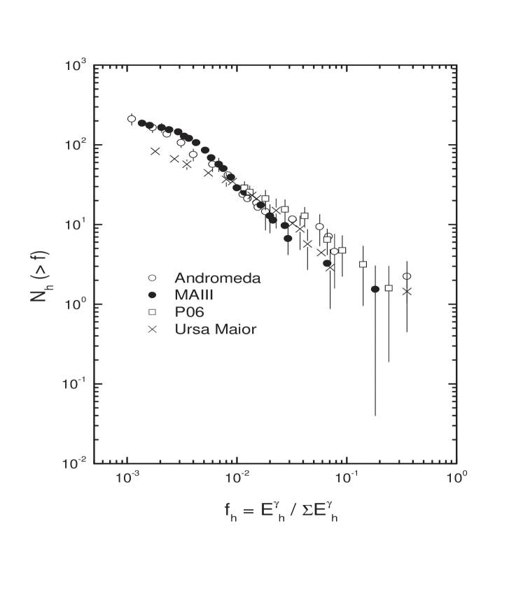
Figure 1: The experimental data of four halo events at Mt. Chacaltaya.

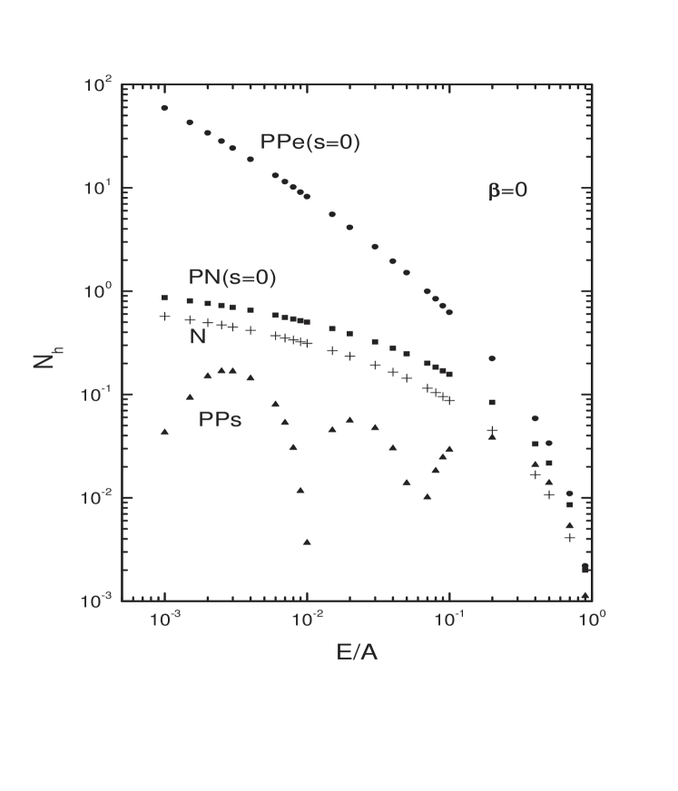
Figure 2: The $\beta=0$ integrated flux of the nucleon (N), the pion from nucleon of the essential residue $s=0$ (PN), the pion from pion of the simple residue (PPs), the pion from pion of the essential residue $s=0$ (PPe).

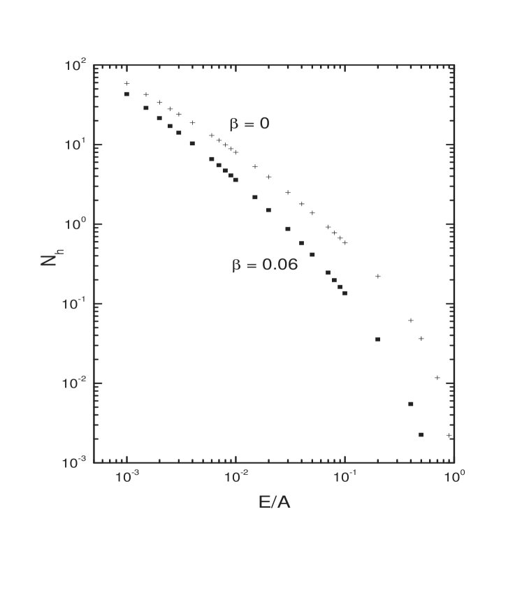
Figure 3: The $\beta=0$ and $\beta=0.06$ total integrated pion flux.

References

- (1) C.M.G. Lattes et al Proc. of the 12th ICRC 7, 2275 (1971).
- (2) N.M. Amato, N. Arata, and R.H.C. Maldonado Il Nuovo Cimento C 10, 559 (1987).
- (3) J.A. Chinellato PhD Thesis University of Campinas, Brazil, 1981.
- (4) S. Yamashita J. Phys. Soc. Japan 54, 529 (1985).
- (5) Pamir Collab. Proc. of the 20th ICRC 5, 383 (1987).
- (6) M. Akashi et al Il Nuovo Cimento A 67, 221 (1982).
- (7) J.R. Ren et al Proc. of the 20th ICRC 5, 375 (1987).
- (8) H. Aoki et al J. Phys. G: Nucl. and Part. Phys. 30, 137 (2004).
- (9) L.N. Capedevielle et al KFK Report 4998 (1992).
- (10) N.N. Kalmikov and S.S. Ostapchenko Yad. Fiz. 56, 105 (1993).
- (11) K. Werner Phys. Rep. 232, 87 (1993).
- (12) N. Amato, E. Shibuya, R.H.C. Maldonado, and H.M. Portella J. Phys. G: Nucl. and Part. Phys. 20, 829 (1994).
-
(13)
K.H. Tsui, H.M. Portella, C.E. Navia, H. Shigueoka,
and L.C.S. de Oliveira
J. Phys. G: Nucl. Part. Phys. 31, 1275 (2005);
K.H. Tsui, H.M. Portella, A.S. Gomes, H. Shigueoka, and L.C.S. de Oliveira Brazilian J. Phys. 37, 419 (2007). - (14) N. Arata and F.M.O. Castro Brazilian J. Phys. 18, 261 (1988).
- (15) N.G. Boyadzhyan, A.P. Garayaka, and E.A. Mamidzhanyan Sov. J. Nucl. Phys. 34, 67 (1981).
- (16) J. Bellandi Filho, S.Q. Brunetto, J.A. Chinellato, R.J.M. Covolan, C. Dobrigkeit, and M.A. Alves Il Nuovo Cimento C 14, 15 (1991).
-
(17)
A. Ohsawa, E.H. Shibuya, and M. Tamada
ICRR-Report-454-99-12 19 (1999);
A. Ohsawa, E.H. Shibuya, and M. Tamada Phys. Rev. D 64, 054004 (2001). - (18) J. D. de Deus Phys. Rev. D 32, 2334 (1985).
-
(19)
A.B. Kaidalov and K.A. Ter-Martyrosian
Phys. Lett. B 117, 247 (1982);
A.B. Kaidalov and K.A. Ter-Martyrosian Sov. J. Nucl. Phys. 40, 135R (1984). -
(20)
G.N. Fowler, A. Vourdas, R.M. Weiner, and G. Wilk
Phys. Rev. D 35, 870 (1987);
G.N. Fowler, F.S. Navarra, M. Plumer, A. Vourdas, R.M. Weiner, and G. Wilk Phys. Rev. C 40, 1219 (1989). - (21) A. Ohsawa and K. Sawayanagi Phys. Rev. D 45, 3128 (1992).
- (22) Z. Wlodarczyk J. Phys. G: Nucl. and Part. Phys. 21, 281 (1995).
- (23) C.R.A. Augusto, S.L.C. Barroso, Y. Fujimoto, V. Kopenkin, M. Moriya, C.E. Navia, A. Ohsawa, E.H. Shibuya, and M. Tamada Phys. Rev. D 61, 012003 (1999).
- (24) A. Ohsawa Prog. Theor. Phys. 92, 1005 (1994).
- (25) H.M. Portella, F.M.O. Castro, and N. Arata J. Phys. G: Nucl. and Part. Phys. 14, 1157 (1988).
- (26) H.M. Portella, H. Shigueoka, A.S. Gomes, and C.E.C. Lima J. Phys. G: Nucl. and Part. Phys. 27, 191 (2001).
- (27) J. Bellandi Filho, S.Q. Brunetto, J.A. Chinellato, C. Dobrigkeit, A. Ohsawa, K. Sawayanagi, and E.H. Shibuya Prog. Theor. Phys. 83, 58 (1990).
- (28) R. Courrant and D. Hilbert Methods of Mathematical Physics Vol. II, Chapter II (Interscience, New York, 1962).
- (29) K.H. Tsui Optics Commun. 90, 283 (1992).
- (30) K.H. Tsui Phys. Fluids B 5, 3808 (1993).
- (31) H.M. Portella, A.S. Gomes, N. Amato, and R.H.C. Maldonado J. Phys. A: Math. and General 31, 6861 (1998).
- (32) H.M. Portella, L.C.S. de Oliveira, and C.E.C. Lima Int. J. Mod. Phys. A 19, 3583 (2004).