Non-linear estimation is easy

Abstract

Non-linear state estimation and some related topics, like parametric estimation, fault diagnosis, and perturbation attenuation, are tackled here via a new methodology in numerical differentiation. The corresponding basic system theoretic definitions and properties are presented within the framework of differential algebra, which permits to handle system variables and their derivatives of any order. Several academic examples and their computer simulations, with on-line estimations, are illustrating our viewpoint.

Non-linear systems, observability, parametric identifiability, closed-loop state estimation, closed-loop parametric identification, closed-loop fault diagnosis, closed-loop fault tolerant control, closed-loop perturbation attenuation, numerical differentiation, differential algebra.

M. Fliess is a Research Director at the Centre National de la Recherche Scientifique and works at the École Polytechnique (Palaiseau, France). He is the head of the INRIA project called ALIEN, which is devoted to the study and the development of new techniques in identification and estimation. In 1991 he invented with J. Lévine, P. Martin, and P. Rouchon, the notion of differentially flat systems which is playing a major rôle in control applications.
C. Join received his Ph.D. degree from the University of Nancy, France, in 2002. He is now an Associate Professor at the University of Nancy and is a member of the INRIA project ALIEN. He is interested in the development of estimation technics for linear and non-linear systems with a peculiar emphasis in fault diagnosis and accommodation. His research involves also signal and image processing.
H. Sira-Ramírez obtained the Electrical Engineer’s degree from the Universidad de Los Andes in Mérida (Venezuela) in 1970. He later obtained the MSc in EE and the Electrical Engineer degree, in 1974, and the PhD degree, also in EE, in 1977, all from the Massachusetts Institute of Technology (Cambridge, USA). Dr. Sira-Ramírez worked for 28 years at the Universidad de Los Andes where he held the positions of: Head of the Control Systems Department, Head of the Graduate Studies in Control Engineering and Vicepresident of the University. Currently, he is a Titular Researcher in the Centro de Investigación y Estudios Avanzados del Instituto Politécnico Nacional (CINVESTAV-IPN) in México City (México). Dr Sira-Ramírez is a Senior Member of the Institute of Electrical and Electronics Engineers (IEEE), a Distinguished Lecturer from the same Institute and a Member of the IEEE International Committee. He is also a member of the Society for Industrial and Applied Mathematics (SIAM), of the International Federation of Automatic Control (IFAC) and of the American Mathematical Society (AMS). He is a coauthor of the books, Passivity Based Control of Euler-Lagrange Systems published by Springer-Verlag, in 1998, Algebraic Methods in Flatness, Signal Processing and State Estimation, Lagares 2003, Differentially Flat Systems, Marcel Dekker, 2004, Control de Sistemas No Lineales Pearson-Prentice Hall 2006, and of Control Design Techniques in Power Electronics Devices, Springer, 2006. Dr. Sira-Ramírez is interested in the theoretical and practical aspects of feedback regulation of nonlinear dynamic systems with special emphasis in Variable Structure feedback control techniques and its applications in Power Electronics.

1 Introduction

1.1 General overview

Since fifteen years non-linear flatness-based control (Fliess, Lévine, Martin & Rouchon (1995, 1999)) has been quite effective in many concrete and industrial applications (see also Lamnabhi-Lagarrigue & Rouchon (2002b); Rudolph (2003); Sira-Ramírez & Agrawal (2004)). On the other hand, most of the problems pertaining to non-linear state estimation, and to related topics, like

• parametric estimation,

• fault diagnosis and fault tolerant control,

• perturbation attenuation,

remain largely open in spite of a huge literature. This paper aims at providing simple and effective design methods for such questions. This is made possible by the following facts:

According to the definition given by Diop & Fliess (1991a, b), a non-linear input-output system is observable if, and only if, any system variable, a state variable for instance, is a differential function of the control and output variables, i.e., a function of those variables and their derivatives up to some finite order. This definition is easily generalized to parametric identifiability and fault isolability. We will say more generally that an unknown quantity may be determined if, and only if, it is expressible as a differential function of the control and output variables.

It follows from this conceptually simple and natural viewpoint that non-linear estimation boils down to numerical differentiation, i.e., to the derivatives estimations of noisy time signals. This classic ill-posed mathematical problem has been already attacked by numerous means. We follow here another thread, which started in Fliess & Sira-Ramírez (2004b) and Fliess, Join, Mboup & Sira-Ramírez (2004, 2005): derivatives estimates are obtained via integrations. This is the explanation of the quite provocative title of this paper where non-linear asymptotic estimators are replaced by differentiators, which are easy to implement.

Remark 1.1.

This approach to non-linear estimation should be regarded as an extension of techniques for linear closed-loop parametric estimation (Fliess & Sira-Ramírez (2003, 2007)). Those techniques gave as a byproduct linear closed-loop fault diagnosis (Fliess, Join & Sira-Ramírez (2004)), and linear state reconstructors (Fliess & Sira-Ramírez (2004a)), which offer a promising alternative to linear asymptotic observers and to Kalman’s filtering.

1.2 Numerical differentiation: a short summary of our approach

.

Let us start with the first degree polynomial time function $p_{1}(t)=a_{0}+a_{1}t$, $t\geq 0$, $a_{0},a_{1}\in\mathbb{R}$. Rewrite thanks to classic operational calculus (see, e.g., Yosida (1984)) $p_{1}$ as $P_{1}=\frac{a_{0}}{s}+\frac{a_{1}}{s^{2}}$. Multiply both sides by $s^{2}$:

$$s^{2}P_{1}=a_{0}s+a_{1}$$ (1)

Take the derivative of both sides with respect to $s$, which corresponds in the time domain to the multiplication by $-t$:

$$s^{2}\frac{dP_{1}}{ds}+2sP_{1}=a_{0}$$ (2)

The coefficients $a_{0},a_{1}$ are obtained via the triangular system of equations (1)-(2). We get rid of the time derivatives, i.e., of $sP_{1}$, $s^{2}P_{1}$, and $s^{2}\frac{dP_{1}}{ds}$, by multiplying both sides of Equations (1)-(2) by $s^{-n}$, $n\geq 2$. The corresponding iterated time integrals are low pass filters which attenuate the corrupting noises, which are viewed as highly fluctuating phenomena (cf. Fliess (2006)). A quite short time window is sufficient for obtaining accurate values of $a_{0}$, $a_{1}$.

The extension to polynomial functions of higher degree is straightforward. For derivatives estimates up to some finite order of a given smooth function $f:[0,+\infty)\to\mathbb{R}$, take a suitable truncated Taylor expansion around a given time instant $t_{0}$, and apply the previous computations. Resetting and utilizing sliding time windows permit to estimate derivatives of various orders at any sampled time instant.

Remark 1.2.

Note that our differentiators are not of asymptotic nature, and do not require any statistical knowledge of the corrupting noises. Those two fundamental features remain therefore valid for our non-linear estimation. This is a change of paradigms when compared to most of today’s approaches.

1.3 Analysis and organization of our paper

Our paper is organized as follows. Section 2 deals with the differential algebraic setting for nonlinear systems, which was introduced in Fliess (1989, 1990). When compared to those expositions and to other ones like Fliess, Lévine, Martin & Rouchon (1995); Delaleau (2002); Rudolph (2003); Sira-Ramírez & Agrawal (2004), the novelty lies in the two following points:

1. The definitions of observability and parametric identifiability are borrowed from Diop & Fliess (1991a, b).

2. We provide simple and natural definitions related to non-linear diagnosis such as detectability, isolability, parity equations, and residuals, which are straightforward extensions of the module-theoretic approach in Fliess, Join & Sira-Ramírez (2004) for linear systems.

The main reason if not the only one for utilizing differential algebra is the absolute necessity of considering derivatives of arbitrary order of the system variables. Note that this could have been also achieved with the differential geometric language of infinite order prolongations (see, e.g., Fliess, Lévine, Martin & Rouchon (1997, 1999)).

Section 3 details Subsection 1.2 on numerical differentiation.

Illustrations are provided by several academic examples and their numerical simulations which we wrote in a such a style that they are easy to grasp without understanding the algebraic subtleties of Section 2:

1. Section 4 is adapting a paper by Fan & Arcak (2003) on a non-linear observer. We only need for closing the loop derivatives of the output signal. We nevertheless present also a state reconstructor of an important physical variable.

2. Closed-loop parametric identification is achieved in Section 5.

3. Section 6 deals with closed-loop fault diagnosis and fault tolerant control.

4. Perturbation attenuation is presented in Section 7, via linear and non-linear case-studies.

We end with a brief conclusion. First drafts of various parts of this paper were presented in Fliess & Sira-Ramírez (2004b); Fliess, Join & Sira-Ramírez (2005).

2 Differential algebra

Commutative algebra, which is mainly concerned with the study of commutative rings and fields, provides the right tools for understanding algebraic equations (see, e.g., Hartshorne (1977); Eisenbud (1995)). Differential algebra, which was mainly founded by Ritt (1950) and Kolchin (1973), extends to differential equations concepts and results from commutative algebra.

2.1 Basic definitions

A differential ring $R$, or, more precisely, an ordinary differential ring, (see, e.g., Kolchin (1973) and Chambert-Loir (2005)) will be here a commutative ring which is equipped with a single derivation $\frac{d}{dt}:R\rightarrow R$ such that, for any $a,b\in R$,

• $\frac{d}{dt}(a+b)=\dot{a}+\dot{b}$,

• $\frac{d}{dt}(ab)=\dot{a}b+a\dot{b}$.

where $\frac{da}{dt}=\dot{a}$, $\frac{d^{\nu}a}{dt^{\nu}}=a^{(\nu)}$, $\nu\geq 0$. A differential field, or, more precisely, an ordinary differential field, is a differential ring which is a field. A constant of $R$ is an element $c\in R$ such that $\dot{c}=0$. A (differential) ring (resp. field) of constants is a differential ring (resp. field) which only contains constants. The set of all constant elements of $R$ is a subring (resp. subfield), which is called the subring (resp.subfield) of constants.

A differential ring (resp. field) extension is given by two differential rings (resp. fields) $R_{1}$, $R_{2}$, such that $R_{1}\subseteq R_{2}$, and qthe derivation of $R_{1}$ is the restriction to $R_{1}$ of the derivation of $R_{2}$.

Notation Let $S$ be a subset of $R_{2}$. Write $R_{1}\{S\}$ (resp. $R_{1}\langle S\rangle$) the differential subring (resp. subfield) of $R_{2}$ generated by $R_{1}$ and $S$.  

Notation Let $k$ be a differential field and $X=\{x_{\iota}|\iota\in I\}$ a set of differential indeterminates, i.e., of indeterminates and their derivatives of any order. Write $k\{X\}$ the differential ring of differential polynomials, i.e., of polynomials belonging to $k[x_{\iota}^{(\nu_{\iota})}|\iota\in I;~{}\nu_{\iota}\geq 0]$. Any differential polynomial is of the form $\sum_{\mbox{\tiny\rm finite}}c\prod_{\mbox{\tiny\rm finite}}(x_{\iota}^{(\mu_{\iota})})^{\alpha_{\mu_{\iota}}}$, $c\in k$.  

Notation If $R_{1}$ and $R_{2}$ are differential fields, the corresponding field extension is often written $R_{2}/R_{1}$.  

A differential ideal $\mathfrak{I}$ of $R$ is an ideal which is also a differential subring. It is said to be prime if, and only if, $\mathfrak{I}$ is prime in the usual sense.

2.2 Field extensions

All fields are assumed to be of characteristic zero. Assume also that the differential field extension $K/k$ is finitely generated, i.e., there exists a finite subset $S\subset K$ such that $K=k\langle S\rangle$. An element $a$ of $K$ is said to be differentially algebraic over $k$ if, and only if, it satisfies an algebraic differential equation with coefficients in $k$: there exists a non-zero polynomial $P$ over $k$, in several indeterminates, such that $P(a,\dot{a},\dots,a^{(\nu)})=0$. It is said to be differentially transcendental over $k$ if, and only if, it is not differentially algebraic. The extension $K/k$ is said to be differentially algebraic if, and only if, any element of $K$ is differentially algebraic over $k$. An extension which is not differentially algebraic is said to be differentially transcendental.

The following result is playing an important rôle:

Proposition 2.1.

The extension $K/k$ is differentially algebraic if, and only if, its transcendence degree is finite.

A set $\{\xi_{\iota}\mid\iota\in I\}$ of elements in $K$ is said to be differentially algebraically independent over $k$ if, and only if, the set $\{\xi^{(\nu)}_{\iota}\mid\iota\in I,\nu\geq 0\}$ of derivatives of any order is algebraically independent over $k$. If a set is not differentially algebraically independent over $k$, it is differentially algebraically dependent over $k$. An independent set which is maximal with respect to inclusion is called a differential transcendence basis. The cardinalities, i.e., the numbers of elements, of two such bases are equal. This cardinality is the differential transcendence degree of the extension $K/k$; it is written $\mbox{\rm diff~{}tr~{}deg }(K/k)$. Note that this degree is $0$ if, and only if, $K/k$ is differentially algebraic.

2.3 Kähler differentials

Kähler differentials (see, e.g., Hartshorne (1977); Eisenbud (1995)) provide a kind of analogue of infinitesimal calculus in commutative algebra. They have been extended to differential algebra by Johnson (1969). Consider again the extension $K/k$. Denote by

• $K[\frac{d}{dt}]$ the set of linear differential operators $\sum_{\text{\rm finite}}a_{\alpha}\frac{d^{\alpha}}{dt^{\alpha}}$, $a_{\alpha}\in K$, which is a left and right principal ideal ring (see, e.g., McConnell & Robson (2000));

• $\Omega_{K/k}$ the left $K[\frac{d}{dt}]$-module of Kähler differentials of the extension $K/k$;

• $d_{K/k}x\in\Omega_{K/k}$ the (Kähler) differential of $x\in K$.

Proposition 2.2.

The next two properties are equivalent:

1. The set $\{x_{\iota}\mid\iota\in I\}\subset K$ is differentially algebraically dependent (resp. independent) over $k$.

2. The set $\{d_{K/k}x_{\iota}\mid\iota\in I\}$ is $K[\frac{d}{dt}]$-linearly dependent (resp. independent).

The next corollary is a direct consequence from Propositions 2.1 and 2.2.

Corollary 2.1.

The module $\Omega_{K/k}$ satisfies the following properties:

• The rank of $\Omega_{K/k}$ is equal to the differential transcendence degree of $K/k$.

• $\Omega_{K/k}$ is torsion if, and only if, $K/k$ is differentially algebraic.

• $\dim_{K}(\Omega_{K/k})=\mbox{\rm tr}~{}\mbox{\rm deg}(L/K)$. It is therefore finite if, and only if, $L/K$ is differentially algebraic.

• $\Omega_{K/k}=\{0\}$ if, and only if, $L/K$ is algebraic.

2.4 Nonlinear systems

2.4.1 Generalities

Let $k$ be a given differential ground field. A (nonlinear) (input-output) system is a finitely generated differential extension $K/k$. Set $K=k\langle S,\bm{\textbf{W}},\bm{\pi}\rangle$ where

1. $S$ is a finite set of system variables, which contains the sets $\bm{u}=(u_{1},\dots,u_{m})$ and $\bm{y}=(y_{1},\dots,y_{p})$ of control and output variables,

2. $\bm{\textbf{W}}=\{\textbf{w}_{1},\dots,\textbf{w}_{q}\}$ denotes the fault variables,

3. $\bm{\pi}=(\pi_{1},\dots,\pi_{r})$ denotes the perturbation, or disturbance, variables.

They satisfy the following properties:

• The control, fault and perturbation variables do not “interact”, i.e., the differential extensions $k\langle\bm{u}\rangle/k$, $k\langle\bm{\textbf{W}}\rangle/k$ and $k\langle\bm{\pi}\rangle/k$ are linearly disjoint.

• The control (resp. fault) variables are assumed to be independent, i.e., $\bm{u}$ (resp. W) is a differential transcendence basis of $k\langle\bm{u}\rangle/k$ (resp. $k\langle\bm{\textbf{W}}\rangle/k$).

• The extension $K/k\langle\bm{{u}},\bm{\textbf{W}},\bm{\pi}\rangle$ is differentially algebraic.

• Assume that the differential ideal $(\bm{\pi})\subset k\{S,\bm{\pi},\bm{\textbf{W}}\}$ generated by $\bm{\pi}$ is prime. Write

  $$k\{S^{\text{nom}},\bm{\textbf{W}}^{\text{nom}}\}=k\{S,\bm{\pi},\bm{\textbf{W}}\}/(\bm{\pi})$$

  the quotient differential ring, where the nominal system and fault variables $S^{\text{nom}}$, $\bm{\textbf{W}}^{\text{nom}}$ are the canonical images of $S$, W. To those nominal variables corresponds the nominal system $K^{\text{nom}}/k$, where $K^{\text{nom}}=k\langle S^{\text{nom}},\bm{\textbf{W}}^{\text{nom}}\rangle$ is the quotient field of $k\{S^{\text{nom}},\bm{\textbf{W}}^{\text{nom}}\}$, which is an integral domain, i.e., without zero divisors. The extension $K^{\text{nom}}/k\langle\bm{u}^{\text{nom}},\bm{\textbf{W}}^{\text{nom}}\rangle$ is differentially algebraic.

• Assume as above that the differential ideal $(\bm{\textbf{W}}^{\text{nom}})~{}\subset k\{S^{\text{nom}},\bm{\textbf{W}}^{\text{nom}}\}$ generated by $\bm{\textbf{W}}^{\text{nom}}$ is prime. Write

  $$k\{S^{\text{pure}}\}=k\{S^{\text{nom}},\bm{\textbf{W}}^{\text{nom}}\}/(\bm{\textbf{W}}^{\text{nom}})$$

  where the pure system variables $S^{\text{pure}}$ are the canonical images of $S^{\text{nom}}$. To those pure variables corresponds the pure system $K^{\text{pure}}/k$, where $K^{\text{pure}}=k\langle S^{\text{pure}}\rangle$ is the quotient field of $k\{S^{\text{pure}}\}$. The extension $K^{\text{pure}}/k\langle\bm{u}^{\text{pure}}\rangle$ is differentially algebraic.

Remark 2.1.

We make moreover the following natural assumptions: $\mbox{\rm diff~{}tr~{}deg }(k\langle\bm{{u}}^{\rm pure}\rangle/k)=\mbox{\rm diff~{}tr~{}deg }(k\langle\bm{{u}}^{\rm nom}\rangle/k)=\mbox{\rm diff~{}tr~{}deg }(k\langle\bm{{u}}\rangle/k)=m$, $\mbox{\rm diff~{}tr~{}deg }(k\langle\bm{\textbf{W}}^{\rm nom}\rangle/k)=\mbox{\rm diff~{}tr~{}deg }(k\langle\bm{\textbf{W}}\rangle/k)=q$

Remark 2.2.

Remember that differential algebra considers algebraic differential equations, i.e., differential equations which only contain polynomial functions of the variables and their derivatives up to some finite order. This is of course not always the case in practice. In the example of Section 4, for instance, appears the transcendental function $\sin\theta_{l}$. As already noted in Fliess, Lévine, Martin & Rouchon (1995), we recover algebraic differential equations by introducing $\tan\frac{\theta_{l}}{2}$.

2.4.2 State-variable representation

We know, from proposition 2.1, that the transcendence degree of the extension $K/k\langle\bm{\textbf{u}},\bm{\textbf{W}},\bm{\pi}\rangle$ is finite, say $n$. Let $\bm{x}=(x_{1},\dots,x_{n})$ be a transcendence basis. Any derivative $\dot{x}_{i}$, $i=1,\dots,n$, and any output variable $y_{j}$, $j=1,\dots,p$, are algebraically dependent over $k\langle\bm{\textbf{u}},\bm{\textbf{W}},\bm{\pi}\rangle$ on $\bm{x}$:

$$\begin{array}[]{l}A_{i}(\dot{x}_{i},\bm{x})=0\quad i=1,\dots,n\\ B_{j}(y_{j},\bm{x})=0\quad j=1,\dots,p\end{array}$$ (3)

where $A_{i}\in k\langle\bm{\textbf{u}},\bm{\textbf{W}},\bm{\pi}\rangle[\dot{x}_{i},\bm{x}]$, $B_{j}\in k\langle\bm{\textbf{u}},\bm{\textbf{W}},\bm{\pi}\rangle[y_{j},\bm{x}]$, i.e., the coefficients of the polynomials $A_{i}$, $B_{j}$ depend on the control, fault and perturbation variables and on their derivatives up to some finite order.

Eq. (3) becomes for the nominal system

$$\begin{array}[]{l}A^{\text{nom}}_{i}(\dot{x}^{\text{nom}}_{i},\bm{x}^{\text{nom}})=0\quad i=1,\dots,n_{\text{nom}}\leq n\\ B^{\text{nom}}_{j}(y^{\text{nom}}_{j},\bm{x}^{\text{nom}})=0\quad j=1,\dots,p\end{array}$$ (4)

where $A^{\text{nom}}_{i}\in k\langle\bm{\textbf{u}}^{\text{nom}},\bm{\textbf{W}}^{\text{nom}}\rangle[\dot{x}^{\text{nom}}_{i},\bm{x}^{\text{nom}}]$, $B^{\text{nom}}_{j}\in k\langle\bm{\textbf{u}}^{\text{nom}},\bm{\textbf{W}}^{\text{nom}}\rangle[y_{j}^{\text{nom}},\bm{x}^{\text{nom}}]$, i.e., the coefficients of $A^{\text{nom}}_{i}$ and $B^{\text{nom}}_{j}$ depend on the nominal control and fault variables and their derivatives and no more on the perturbation variables and their derivatives.

We get for the pure system

$$\begin{array}[]{l}A^{\text{pure}}_{i}(\dot{x}^{\text{pure}}_{i},\bm{x}^{\text{pure}})=0\quad i=1,\dots,n_{\text{pure}}\leq n_{\text{nom}}\\ B^{\text{pure}}_{j}(y^{\text{pure}}_{j},\bm{x}^{\text{pure}})=0\quad j=1,\dots,p\end{array}$$ (5)

where $A^{\text{pure}}_{i}\in k\langle\bm{\textbf{u}}^{\text{pure}}\rangle[\dot{x}^{\text{pure}}_{i},\bm{x}^{\text{pure}}]$, $B^{\text{pure}}_{j}\in k\langle\bm{\textbf{u}}^{\text{pure}}\rangle[y^{\text{pure}}_{j},\bm{x}^{\text{pure}}]$, i.e., the coefficients of $A^{\text{pure}}_{i}$ and $B^{\text{pure}}_{j}$ depend only on the pure control variables and their derivatives.

Remark 2.3.

Two main differences, which are confirmed by concrete examples (see, e.g., Fliess & Hasler (1990); Fliess, Lévine & Rouchon (1993)), can be made with the usual state-variable representation

$$\begin{array}[]{l}\dot{\bm{x}}=F(\bm{x},\bm{u})\\ \bm{y}=H(\bm{x})\end{array}$$

1. The representations (3), (4), (5) are implicit.

2. The derivatives of the control variables in the equations of the dynamics cannot be in general removed (see Delaleau & Respondek (1995)).

2.5 Variational system

Call $\Omega_{K/k}$ (resp. $\Omega_{K^{\text{nom}}/k}$, $\Omega_{K^{\text{pure}}/k}$) the variational, or linearized, system (resp. nominal system, pure system) of system $K/k$. Proposition 2.2 yields for pure systems

$$A\left(\begin{array}[]{c}d_{K^{\text{pure}}/k}y^{\text{pure}}_{1}\\ \vdots\\ d_{K^{\text{pure}}/k}y^{\text{pure}}_{p}\end{array}\right)=B\left(\begin{array}[]{c}d_{K^{\text{pure}}/k}u^{\text{pure}}_{1}\\ \vdots\\ d_{K^{\text{pure}}/k}u^{\text{pure}}_{m}\end{array}\right)$$ (6)

where

• $A\in K[\frac{d}{dt}]^{p\times p}$ is of full rank,

• $B\in K[\frac{d}{dt}]^{p\times m}$.

The pure transfer matrix is the matrix $A^{-1}B\in K(s)^{p\times m}$, where $K(s)$, $s=\frac{d}{dt}$, is the skew quotient field of $K[\frac{d}{dt}]$.

2.6 Differential flatness

The system $K/k$ is said to be (differentially) flat if, and only if, the pure system $K^{\text{pure}}/k$ is (differentially) flat (Fliess, Lévine, Martin & Rouchon (1995)): the algebraic closure $\bar{K}^{\text{pure}}$ of $K^{\text{pure}}$ is equal to the algebraic closure of a purely differentially transcendental extension of $k$. It means in other words that there exists a finite subset $\bm{z}^{\text{pure}}=\{z_{1}^{\text{pure}},\dots,z_{m}^{\text{pure}}\}$ of $\bar{K}^{\text{pure}}$ such that

• $z_{1}^{\text{pure}},\dots,z_{m}^{\text{pure}}$ are differentially algebraically independent over $k$,

• $z_{1}^{\text{pure}},\dots,z_{m}^{\text{pure}}$ are algebraic over $K^{\text{pure}}$,

• any pure system variable is algebraic over $k\langle z_{1}^{\text{pure}},\dots,z_{m}^{\text{pure}}\rangle$.

$\bm{z}^{\text{pure}}$ is a (pure) flat, or linearizing, output. For a flat dynamics, it is known that the number $m$ of its elements is equal to the number of independent control variables.

2.7 Observability and identifiability

Take a system $K/k$ with control $\bm{u}$ and output $\bm{y}$.

2.7.1 Observability

According to Diop & Fliess (1991a, b) (see also Diop (2002)), system $K/k$ is said to be observable if, and only if, the extension $K^{\text{pure}}/k\langle\bm{u}^{\text{pure}},\bm{y}^{\text{pure}}\rangle$ is algebraic.

Remark 2.4.

This new definition of observability is “roughly” equivalent (see Diop & Fliess (1991a, b) for details) to its usual differential geometric counterpart due to Hermann & Krener (1977) (see also Conte, Moog & Perdon (1999); Gauthier & Kupka (2001); Isidori (1995); Nijmeijer & van der Schaft (1990); Sontag (1998)).

2.7.2 Identifiable parameters

Set $k=k_{0}\langle\mathbf{\Theta}\rangle$, where $k_{0}$ is a differential field and $\mathbf{\Theta}=\{\theta_{1},\dots,\theta_{r}\}$ a finite set of unknown parameters, which might not be constant. According to Diop & Fliess (1991a, b), a parameter $\theta_{\iota}$, $\iota=1,\dots,r$, is said to be algebraically (resp. rationally) identifiable if, and only if, it is algebraic over (resp. belongs to) $k_{0}\langle\bm{u},\bm{y}\rangle$:

• $\theta_{\iota}$ is rationally identifiable if, and only if, it is equal to a differential rational function over $k_{0}$ of the variables $\bm{u}$, $\bm{y}$, i.e., to a rational function of $\bm{u}$, $\bm{y}$ and their derivatives up to some finite order, with coefficients in $k_{0}$;

• $\theta_{\iota}$ is algebraically identifiable if, and only if, it satisfies an algebraic equation with coefficients in $k_{0}\langle\bm{u},\bm{y}\rangle$.

2.7.3 Determinable variables

More generally, a variable $\Upsilon\in K$ is said to be rationally (resp. algebraically) determinable if, and only if, $\Upsilon^{\text{pure}}$ belongs to (resp. is algebraic over) $k\langle\bm{u}^{\text{pure}},\bm{y}^{\text{pure}}\rangle$. A system variable $\chi$ is then said to be rationally (resp. algebraically) observable if, and only if, $\chi^{\text{pure}}$ belongs to (resp. is algebraic over) $k\langle\bm{u}^{\text{pure}},\bm{y}^{\text{pure}}\rangle$.

Remark 2.5.

In the case of algebraic determinability, the corresponding algebraic equation might possess several roots which are not easily discriminated (see, e.g., Li, Chiasson, Bodson & Tolbert (2006) for a concrete example).

Remark 2.6.

See Sedoglavic (2002) and Ollivier & Sedoglavic (2002) for efficient algorithms in order to test observability and identifiability. Those algorithms may certainly be extended to determinable variables and to various questions related to fault diagnosis in Section 2.8.

2.8 Fundamental properties of fault variables

2.8.1 Detectability

The fault variable $\textbf{w}_{\iota}$, $\iota=1,\dots,q$, is said to be detectable if, and only if, the field extension $K^{\text{nom}}/k\langle\bm{u}^{\text{nom}},\bm{\textbf{W}}^{\text{nom}}_{\iota}\rangle$, where $\bm{\textbf{W}}^{\text{nom}}_{\iota}=\bm{\textbf{W}}^{\text{nom}}\backslash\{\textbf{w}^{\text{nom}}_{\iota}\}$, is differentially transcendental. It means that $\textbf{w}_{\iota}$ is indeed “influencing” the output. When considering the variational nominal system, formula (6) yields

$$\begin{array}[]{cl}\left(\begin{array}[]{c}d_{K^{\rm nom}/k}{y}_{1}^{\rm nom}\\ \vdots\\ d_{K^{\rm nom}/k}{y}_{p}^{\rm nom}\end{array}\right)=&T_{\bm{u}}\left(\begin{array}[]{c}d_{K^{\rm nom}/k}{u}_{1}^{\rm nom}\\ \vdots\\ d_{K^{\rm nom}/k}{u}_{m}^{\rm nom}\end{array}\right)\\ &+T_{\bm{\textbf{W}}}\left(\begin{array}[]{c}d_{K^{\rm nom}/k}{\textbf{w}}_{1}^{\rm nom}\\ \vdots\\ d_{K^{\rm nom}/k}{\textbf{w}}_{q}^{\rm nom}\end{array}\right)\end{array}$$

where $T_{\bm{u}}\in K(s)^{p\times m}$, $T_{\bm{\textbf{W}}}\in K(s)^{p\times q}$. Call $T_{\bm{\textbf{W}}}$ the fault transfer matrix. The next result is clear:

Proposition 2.3.

The fault variable $\textbf{w}_{\iota}$ is detectable if, and only if, the $\iota^{th}$ column of the fault transfer matrix $T_{\bm{\textbf{W}}}$ is non-zero.

2.8.2 Isolability, parity equations and residuals

A subset $\bm{\textbf{W}}^{\prime}=(\textbf{w}_{\iota_{1}},\dots,\textbf{w}_{\iota_{q^{\prime}}})$ of the set W of fault variables is said to be

• Differentially algebraically isolable if, and only if, the extension $k\langle\bm{u}^{\rm nom},\bm{y}^{\rm nom},\bm{\textbf{W}}^{\prime\rm nom}\rangle/k\langle\bm{u}^{\rm nom},\bm{y}^{\rm nom}\rangle$ is differentially algebraic. It means that any component of $\bm{\textbf{W}}^{\prime\rm nom}$ satisfies a parity differential equation, i.e., an algebraic differential equations where the coefficients belong to $k\langle\bm{u}^{\rm nom},\bm{y}^{\rm nom}\rangle$.

• Algebraically isolable if, and only if, the extension $k\langle\bm{u}^{\rm nom},\bm{y}^{\rm nom},\bm{\textbf{W}}^{\prime\rm nom}\rangle/k\langle\bm{u}^{\rm nom},\bm{y}^{\rm nom}\rangle$ is algebraic. It means that the parity differential equation is of order $0$, i.e., it is an algebraic equation with coefficients $k\langle\bm{u}^{\rm nom},\bm{y}^{\rm nom}\rangle$.

• Rationally isolable if, and only if, $\bm{\textbf{W}}^{\prime\rm nom}$ belongs to $k\langle\bm{u}^{\rm nom},\bm{y}^{\rm nom}\rangle$. It means that the parity equation is a linear algebraic equation, i.e., any component of $\bm{\textbf{W}}^{\prime\rm nom}$ may be expressed as a rational function over $k$ in the variables $\bm{u}^{\rm nom}$, $\bm{y}^{\rm nom}$ and their derivatives up to some finite order.

The next property is obvious:

Proposition 2.4.

Rational isolability $\Rightarrow$ algebraic isolability $\Rightarrow$ differentially algebraic isolability.

When we will say for short that fault variables are isolable, it will mean that they are differentially algebraically isolable.

Proposition 2.5.

Assume that the fault variables belonging to ${\mbox{\rm}{\bm{\textbf{W}}^{\prime}}}$ are isolable. Then ${\mbox{\rm card}}(\bm{\textbf{W}}^{\prime})\leq\mbox{\rm card}(\bm{y})$.

Proof.

The differential transcendence degree of the extension $k\langle\bm{u}^{\rm nom},\bm{y}^{\rm nom},\bm{\textbf{W}}^{\prime\rm nom}\rangle/k$ (resp. $k\langle\bm{u}^{\rm nom},\bm{y}^{\rm nom}\rangle/k$) is equal to $\mbox{\rm card}(\bm{u})+\mbox{\rm card}(\bm{W}^{\prime})$ (resp. is less than or equal to $\mbox{\rm card}(\bm{u})+\mbox{\rm card}(\bm{y})$). The equality of those two degrees implies our result thanks to the Remark 2.1. ∎

3 Derivatives of a noisy signal

3.1 Polynomial time signals

Consider the real-valued polynomial function $x_{N}(t)=\sum_{\nu=0}^{N}x^{(\nu)}(0)\frac{t^{\nu}}{\nu!}\in\mathbb{R}[t]$, $t\geq 0$, of degree $N$. Rewrite it in the well known notations of operational calculus:

$$X_{N}(s)=\sum_{\nu=0}^{N}\frac{x^{(\nu)}(0)}{s^{\nu+1}}$$

We know utilize $\frac{d}{ds}$, which is sometimes called the algebraic derivative (cf. Mikusinski (1983); Mikusinski & Boehme (1987)). Multiply both sides by $\frac{d^{\alpha}}{ds^{\alpha}}s^{N+1}$, $\alpha=0,1,\dots,N$. The quantities $x^{(\nu)}(0)$, $\nu=0,1,\dots,N$ are given by the triangular system of linear equations:

$$\frac{d^{\alpha}s^{N+1}X_{N}}{ds^{\alpha}}=\frac{d^{\alpha}}{ds^{\alpha}}\left(\sum_{\nu=0}^{N}x^{(\nu)}(0)s^{N-\nu}\right)$$ (7)

The time derivatives, i.e., $s^{\mu}\frac{d^{\iota}X_{N}}{ds^{\iota}}$, $\mu=1,\dots,N$, $0\leq\iota\leq N$, are removed by multiplying both sides of Eq. (7) by $s^{-\bar{N}}$, $\bar{N}>N$.

Remark 3.1.

Remember (cf. Mikusinski (1983); Mikusinski & Boehme (1987); Yosida (1984)) that $\frac{d}{ds}$ corresponds in the time domain to the multiplication by $-t$.

3.2 Analytic time signals

Consider a real-valued analytic time function defined by the convergent power series $x(t)=\sum_{\nu=0}^{\infty}x^{(\nu)}(0)\frac{t^{\nu}}{\nu!}$, where $0\leq t<\rho$. Introduce its truncated Taylor expansion

$$x(t)=\sum_{\nu=0}^{N}x^{(\nu)}(0)\frac{t^{\nu}}{\nu!}+O(t^{N+1})$$ (8)

Approximate $x(t)$ in the interval $(0,\varepsilon)$, $0<\varepsilon\leq\rho$, by its truncated Taylor expansion $x_{N}(t)=\sum_{\nu=0}^{N}x^{(\nu)}(0)\frac{t^{\nu}}{\nu!}$ of order $N$. Introduce the operational analogue of $x(t)$, i.e., $X(s)=\sum_{\nu\geq 0}\frac{x^{(\nu)}(0)}{s^{\nu+1}}$, which is an operationally convergent series in the sense of Mikusinski (1983); Mikusinski & Boehme (1987). Denote by $[x^{(\nu)}(0)]_{e_{N}}(t)$, $0\leq\nu\leq N$, the numerical estimate of $x^{(\nu)}(0)$, which is obtained by replacing $X_{N}(s)$ by $X(s)$ in Eq. (7). The next result, which is elementary from an analytic standpoint, provides a mathematical justification for the computer implementations:

Proposition 3.1.

For $0<t<\varepsilon$,

$$\lim_{t\downarrow 0}[x^{(\nu)}(0)]_{e_{N}}(t)=\lim_{N\to+\infty}[x^{(\nu)}(0)]_{e_{N}}(t)=x^{(\nu)}(0)$$ (9)

Proof.

Following (8) replace $x_{N}(t)$ by $x(t)=x_{N}(t)+O(t^{N+1})$. The quantity $O(t^{N+1})$ becomes negligible if $t\downarrow 0$ or $N\to+\infty$. ∎

Remark 3.2.

See Mboup, Join & Fliess (2007)) for fundamental theoretical developments. See also Nöthen (2007) for most fruitful comparisons and discussions.

3.3 Noisy signals

Assume that our signals are corrupted by additive noises. Those noises are viewed here as highly fluctuating, or oscillatory, phenomena. They may be therefore attenuated by low-pass filters, like iterated time integrals. Remember that those iterated time integrals do occur in Eq. (7) after multiplying both sides by $s^{-\bar{N}}$, for $\bar{N}>0$ large enough.

Remark 3.3.

The estimated value of $x(0)$, which is obtained along those lines, should be viewed as a denoising of the corresponding signal.

Remark 3.4.

See Fliess (2006) for a precise mathematical foundation, which is based on nonstandard analysis. A highly fluctuating function of zero mean is then defined by the following property: its integral over a finite time interval is infinitesimal, i.e., “very small”. Let us emphasize that this approach, which has been confirmed by numerous computer simulations and several laboratory experiments in control and in signal processing, is independent of any probabilistic setting. No knowledge of the statistical properties of the noises is required.

4 Feedback and state reconstructor

4.1 System description

Consider with Fan & Arcak (2003) the mechanical system, depicted in Figure 1. It consists of a DC-motor joined to an inverted pendulum through a torsional spring:

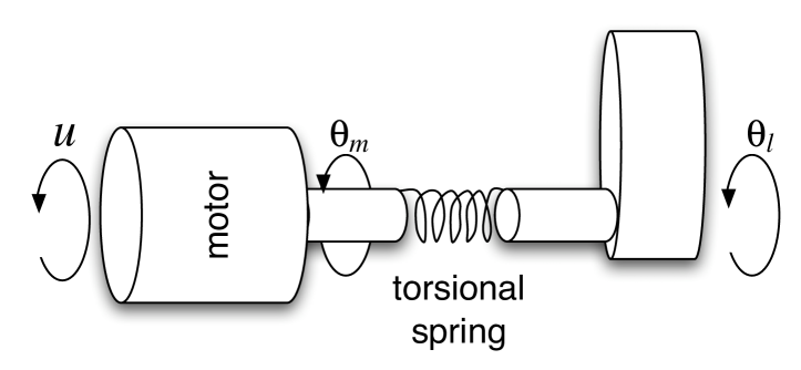
Figure 1: A single link flexible joint manipulator

$$\begin{array}[]{rl}J_{m}\ddot{\theta}_{m}(t)&=\kappa\big{(}\theta_{l}(t)-\theta_{m}(t)\big{)}-B\dot{\theta}_{m}(t)+K_{\tau}u(t)\\ J_{l}\ddot{\theta}_{l}(t)&=-\kappa\big{(}\theta_{l}(t)-\theta_{m}(t)\big{)}-mgh\sin(\theta_{l}(t))\\ y(t)&=\theta_{l}(t)\end{array}$$ (10)

where

• $\theta_{m}$ and $\theta_{l}$ represent respectively the angular deviation of the motor shaft and the angular position of the inverted pendulum,

• $J_{m}$, $J_{l}$, $h$, $m$, $\kappa$, $B$, $K_{\tau}$ and $g$ are physical parameters which are assumed to be constant and known.

System (10), which is linearizable by static state feedback, is flat; $y=\theta_{l}$ is a flat output.

4.2 Control design

Tracking of a given smooth reference trajectory $y^{\ast}(t)=\theta^{\ast}_{l}(t)$ is achieved via the linearizing feedback controller

$$\begin{array}[]{rl}u(t)&=\frac{1}{K_{\tau}}\Big{(}\frac{J_{m}}{\kappa}\big{[}J_{l}v(t)+\kappa\ddot{y}_{e}(t)\\ &+mgh(\ddot{y}_{e}(t)\cos(y_{e}(t))-(\dot{y}_{e}(t))^{2}\sin(y_{e}(t)))\big{]}\\ &+J_{l}\ddot{y}_{e}(t)+mgh\sin(y_{e}(t))\\ &\frac{B}{\kappa}\big{[}J_{l}y^{(3)}_{e}(t)+\kappa\dot{y}_{e}(t)+mgh\dot{y}_{e}(t)\cos(y_{e}(t)\big{]}\Big{)}\end{array}$$ (11)

where

$$\begin{array}[]{rl}v(t)&=y^{\ast(4)}(t)-\gamma_{4}(y_{e}^{(3)}(t)-y^{\ast(3)}(t))\\ &-\gamma_{3}(\ddot{y}_{e}(t)-\ddot{y}^{\ast}(t))-\gamma_{2}(\dot{y}_{e}(t)-\dot{y}^{\ast}(t))\\ &-\gamma_{1}(y_{e}(t)-y^{\ast}(t))\\ \end{array}$$ (12)

The subscript “$e$”denotes the estimated value. The design parameters $\gamma_{1}$, …, $\gamma_{4}$ are chosen so that the resulting characteristic polynomial is Hurwitz.

Remark 4.1.

Feedback laws like (11)-(12) depend, as usual in flatness-based control (see, e.g., Fliess, Lévine, Martin & Rouchon (1995, 1999); Sira-Ramírez & Agrawal (2004)), on the derivatives of the flat output and not on the state variables.

4.3 A state reconstructor

We might nevertheless be interested in obtaining an estimate $[\theta_{m}]_{e}(t)$ of the unmeasured state $\theta_{m}(t)$:

$$[\theta_{m}]_{e}(t)=\frac{1}{\kappa}\Big{(}J_{l}\ddot{y}_{e}(t)+mgh\sin(y_{e}(t))\Big{)}+y_{e}(t)$$ (13)

4.4 Numerical simulations

The physical parameters have the same numerical values as in Fan & Arcak (2003): $J_{m}=3.7\times 10^{-3}\textit{ kgm${}^{2}$}$, $J_{l}=9.3\times 10^{-3}\textit{ kgm${}^{2}$}$, $h=1.5\times 10^{-1}\textit{ m}$, $m=0.21\textit{ kg}$, $B=4.6\times 10^{-2}\textit{ m}$, $K_{\tau}=8\times 10^{-2}\textit{ NmV${}^{-1}$}$. The numerical simulations are presented in Figures 2 - 9. Robustness has been tested with an additive white Gaussian noise N(0; 0.01) on the output $y$. Note that the off-line estimations of $\ddot{y}$ and $\theta_{m}$, where a “small” delay is allowed, are better than the on-line estimation of $\ddot{y}$.

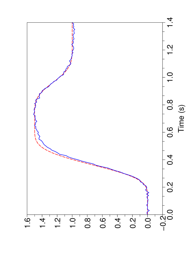
Figure 2: Output (–) and reference trajectory (- -)

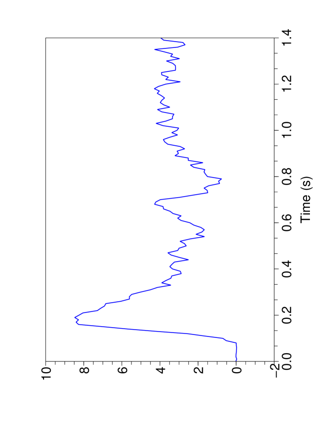
Figure 3: Control

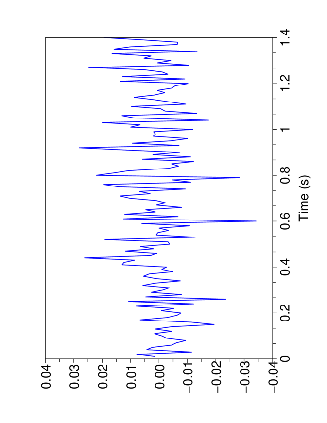
Figure 4: Output noise

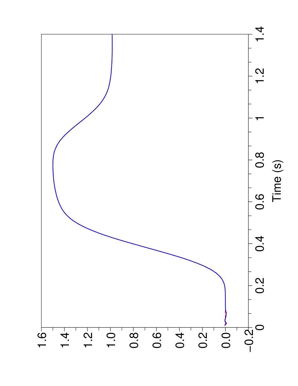
Figure 5: $y$: (- -); on-line noise attenuation $y_{e}$ (–)

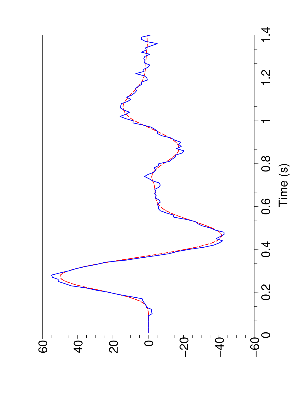
Figure 6: $\ddot{y}$ (- -); on-line estimation $\ddot{y}_{e}$ (–)

,

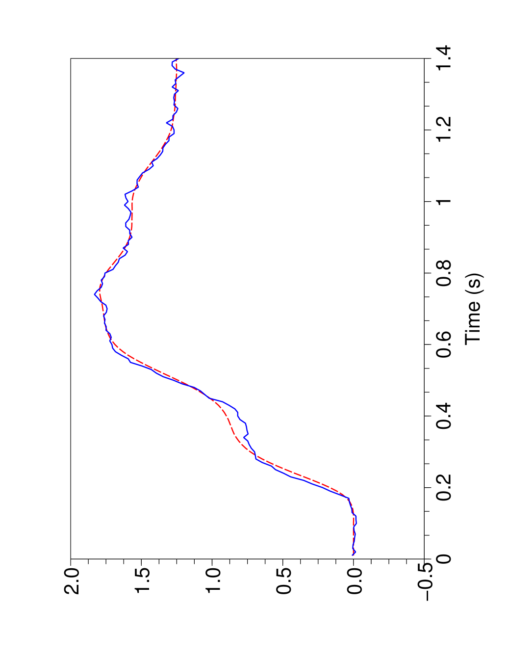
Figure 7: $\theta_{m}$ (- -); on-line estimation $\text{[}\theta_{m}\text{]}_{e}$ (–)

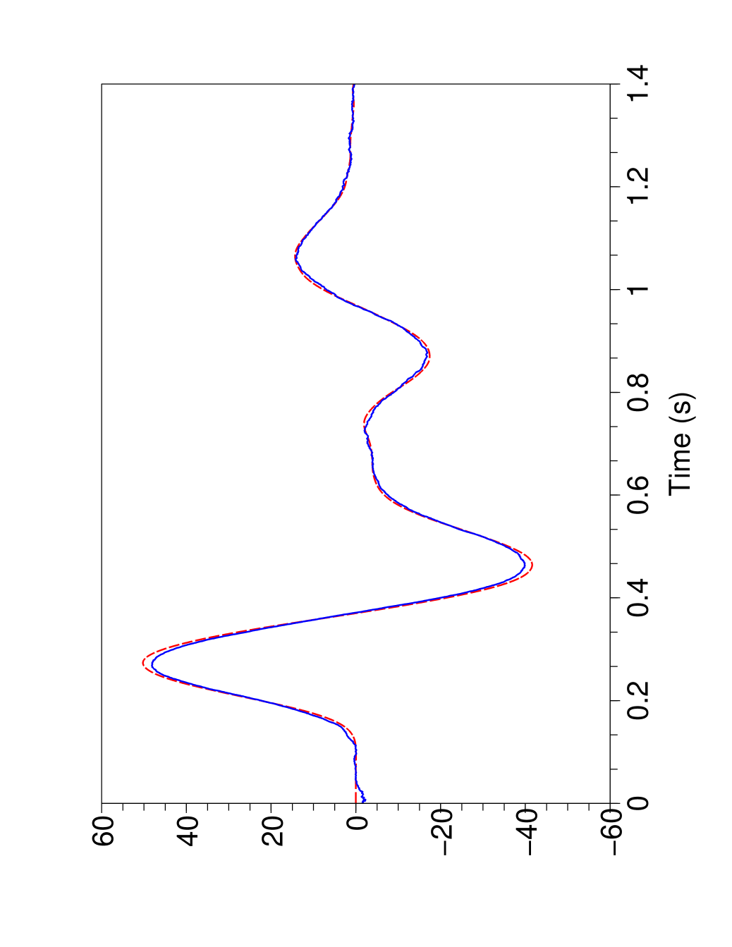
Figure 8: $\ddot{y}$ (- -); off-line estimation $\ddot{y}_{e}$ (–)

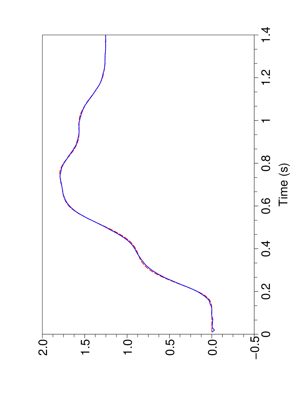
Figure 9: $\theta_{m}$ (- -); off-line estimation $\text{[}\theta_{m}\text{]}_{e}$ (–)

5 Parametric identification

5.1 A rigid body

Consider the fully actuated rigid body, depicted in Figure 10, which is given by the Euler equations

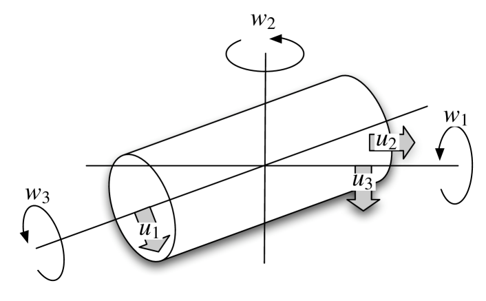
Figure 10: Rigid body

$$\begin{array}[]{rl}I_{1}\dot{w}_{1}(t)=(I_{2}-I_{3})w_{2}(t)w_{3}(t)+u_{1}(t)\\ I_{2}\dot{w}_{2}(t)=(I_{3}-I_{1})w_{3}(t)w_{1}(t)+u_{2}(t)\\ I_{3}\dot{w}_{3}(t)=(I_{1}-I_{2})w_{1}(t)w_{2}(t)+u_{3}(t)\\ \end{array}$$ (14)

where $w_{1}$, $w_{2}$, $w_{3}$ are the measured angular velocities, $u_{1}$, $u_{2}$, $u_{3}$ the applied control input torques, $I_{1}$, $I_{2}$, $I_{3}$ the constant moments of inertia, which are poorly known. System (14) is stabilized around the origin, for suitably chosen design parameters $\lambda_{1\iota}$, $\lambda_{0\iota}$, $\iota=1,2,3$, by the feedback controller, which is an obvious extension of the familiar proportional-integral (PI) regulators,

$$\begin{array}[]{rl}u_{1}(t)=&-(I_{2}-I_{3})w_{2}(t)w_{3}(t)\\ &+I_{1}\Big{(}-\lambda_{11}w_{1}(t)-\lambda_{01}\int_{0}^{t}w_{1}(\sigma)d\sigma\Big{)}\\ u_{2}(t)=&-(I_{3}-I_{1})w_{3}(t)w_{1}(t)\\ &+I_{2}\Big{(}-\lambda_{12}w_{2}(t)-\lambda_{02}\int_{0}^{t}w_{2}(\sigma)d\sigma\Big{)}\\ u_{3}(t)=&-(I_{1}-I_{2})w_{1}(t)w_{2}(t)\\ &+I_{3}\Big{(}-\lambda_{13}w_{3}(t)-\lambda_{03}\int_{0}^{t}w_{3}(\sigma)d\sigma\Big{)}\\ \end{array}$$ (15)

5.2 Identification of the moments of inertia

Write Eq. (14) in the following matrix form:

$$\begin{array}[]{l}\begin{pmatrix}\dot{w}_{1}&-w_{2}w_{3}&w_{2}w_{2}\\ w_{1}w_{3}&\dot{w}_{2}&-w_{1}w_{3}\\ -w_{1}w_{2}&w_{1}w_{2}&\dot{w}_{3}\end{pmatrix}\times\\ \begin{pmatrix}I_{1}\\ I_{2}\\ I_{3}\end{pmatrix}=\begin{pmatrix}u_{1}\\ u_{2}\\ u_{3}\end{pmatrix}\end{array}$$

It yields estimates $[I_{1}]_{e}$, $[I_{2}]_{e}$, $[I_{3}]_{e}$ of $I_{1}$, $I_{2}$, $I_{3}$ when we replace $w_{1}$, $w_{2}$, $w_{3}$, $\dot{w}_{1}$, $\dot{w}_{2}$, $\dot{w}_{3}$ by their estimates. The control law (15) becomes

$$\begin{array}[]{rl}u_{1}(t)=&-([I_{2}]_{e}-[I_{3}]_{e})[w_{2}]_{e}(t)[w_{3}]_{e}(t)\\ &+[I_{1}]_{e}\Big{(}-\lambda_{11}[w_{1}]_{e}(t)-\lambda_{01}\int_{0}^{t}[w_{1}]_{e}(\sigma)d\sigma\Big{)}\\ u_{2}(t)=&-([I_{3}]_{e}-[I_{1}]_{e})[w_{3}]_{e}(t)[w_{1}]_{e}(t)\\ &+[I_{2}]_{e}\Big{(}-\lambda_{12}[w_{2}]_{e}(t)-\lambda_{02}\int_{0}^{t}[w_{2}]_{e}(\sigma)d\sigma\Big{)}\\ u_{3}(t)=&-([I_{1}]_{e}-[I_{2}]_{e})[w_{1}]_{e}(t)[w_{2}]_{e}(t)\\ &+[I_{3}]_{e}\Big{(}-\lambda_{13}[w_{3}]_{e}(t)-\lambda_{03}\int_{0}^{t}[w_{3}]_{e}(\sigma)d\sigma\Big{)}\\ \end{array}$$ (16)

5.3 Numerical simulations

The output measurements are corrupted by an additive Gaussian white noise $N(0;0.005)$. Figure 11 shows an excellent on-line estimation of the three moments of inertia. Set for the design parameters in the controllers (15) and (16) $\lambda_{1\iota}=2\xi\varpi$, $\lambda_{0\iota}=\varpi^{2}$, $\iota=1,2,3$, where $\xi=0.707$, $\varpi=0.5$. The stabilization with the above estimated values in Figure 12 is quite better than in Figure 13 where the following false values where utilized: $I_{1}=0.2$, $I_{2}=0.1$ and $I_{3}=0.1$.

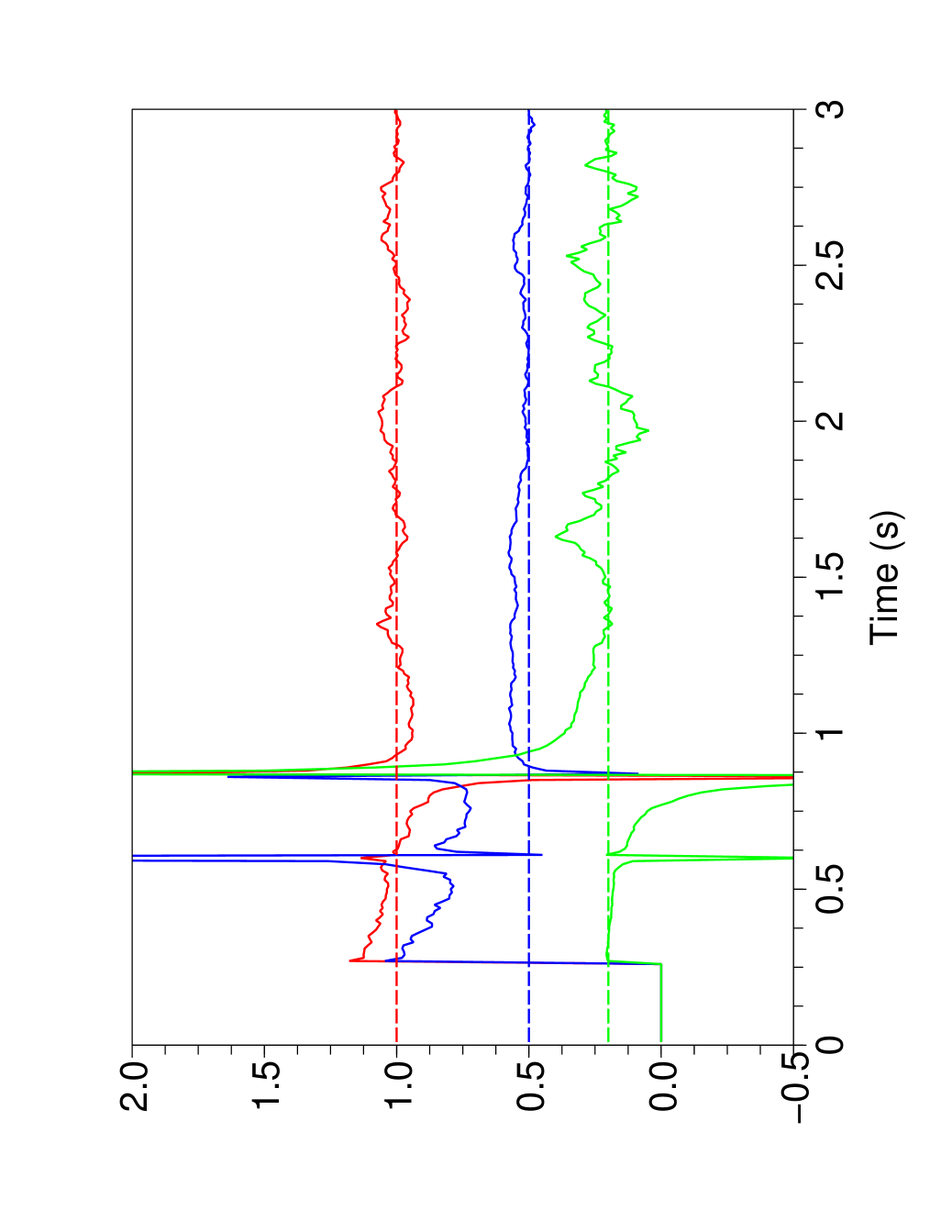
Figure 11: Zoom on the parametric estimation (–) and real values (- -)

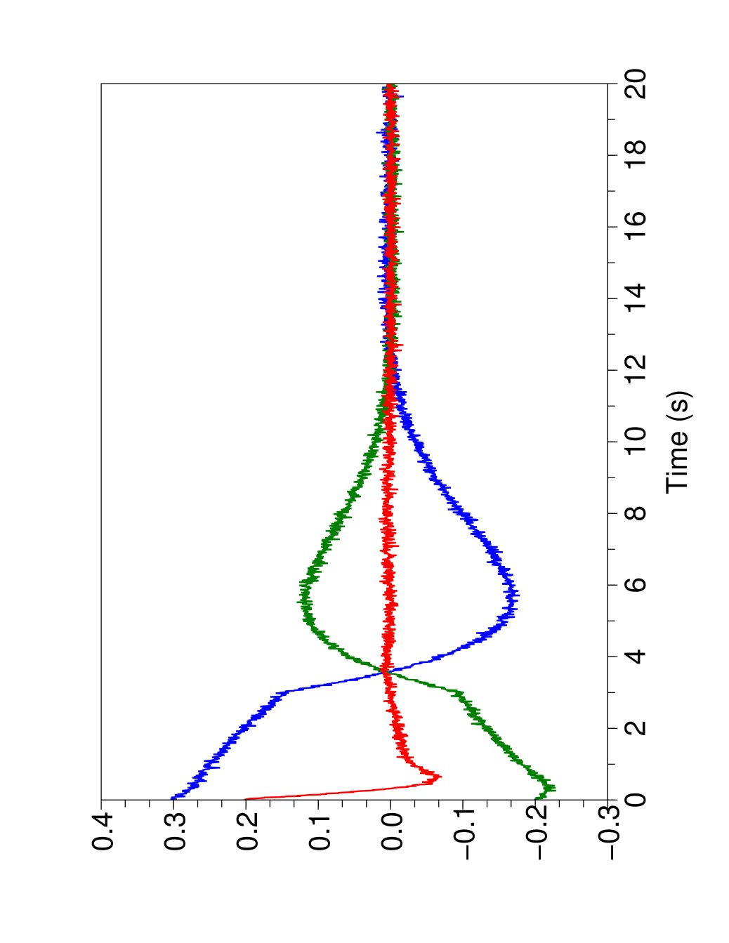
Figure 12: Feedback stabilization with parametric estimation

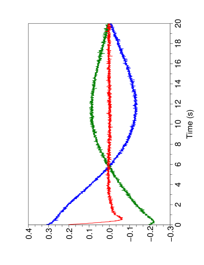
Figure 13: Feedback stabilization without parametric estimation

6 Fault diagnosis and accommodation

6.1 A two tank system

Consider the cascade arrangement of two identical tank systems, shown in Figure 14, which is a popular example in fault diagnosis (see, e.g., Blanke, Kinnaert, Lunze & Staroswiecki (2003)).

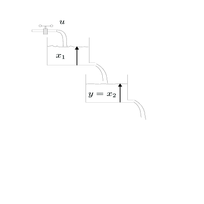
Figure 14: A two tank system

Its mathematical description is given by

$${\dot{x}}_{1}(t) = -\frac{c}{A}\sqrt{x_{1}(t)}+\frac{1}{A}u(t)\left(1-{\bf w}(t)\right)$$ (17)

$$+\varpi(t)$$

$${\dot{x}}_{2}(t) = \frac{c}{A}\sqrt{x_{1}(t)}-\frac{c}{A}\sqrt{x_{2}(t)}$$

$$y(t) = x_{2}(t)$$

where:

• The constant $c$ and the area $A$ of the tank’s bottom are known parameters.

• The perturbation $\varpi(t)$ is constant but unknown,

• The actuator failure ${\bf w}(t)$, $0\leq{\bf w}(t)\leq 1$, is constant but unknown. It starts at some unknown time $t_{I}>>0$ which is not “small”.

• Only the output $y=x_{2}$ is available for measurement.

The corresponding pure system, where we are ignoring the fault and perturbation variables (cf. Section 2.4.1),

$$\begin{array}[]{l}\dot{x}^{\text{pure}}_{1}=-\frac{c}{A}\sqrt{x^{\text{pure}}_{1}}+\frac{1}{A}u^{\text{pure}}\\ \dot{x}^{\text{pure}}_{2}=\frac{c}{A}\sqrt{x^{\text{pure}}_{1}}-\frac{c}{A}\sqrt{x^{\text{pure}}_{2}}\\ y^{\text{pure}}=x^{\text{pure}}_{2}\end{array}$$

is flat. Its flat output is $y^{\text{pure}}=x^{\text{pure}}_{2}$. The state variable $x^{\text{pure}}_{1}$ and control variable $u^{\text{pure}}$ are given by

$$x^{\text{pure}}_{1} = \big{(}\frac{A}{c}{\dot{y}}^{\text{pure}}+\sqrt{y^{\text{pure}}}\big{)}^{2}$$ (18)

$$u^{\text{pure}} = 2A\big{(}\frac{A}{c}{\dot{y}}^{\text{pure}}+\sqrt{y^{\text{pure}}}\big{)}\big{(}\frac{A}{c}{\ddot{y}}^{\text{pure}}+\frac{{\dot{y}}^{\text{pure}}}{2\sqrt{y^{\text{pure}}}}\big{)}$$ (19)

$$+c\big{(}\frac{A}{c}{\dot{y}}^{\text{pure}}+\sqrt{y^{\text{pure}}}\big{)}$$

6.2 Fault tolerant tracking controller

It is desired that the output $y$ tracks a given smooth reference trajectory $y^{\ast}(t)$. Rewrite Formulae (18)-(19) by taking into account the perturbation variable $\varpi(t)$ and the actuator failure ${\bf w}(t)$:

$$x_{1}(t) = \big{(}\frac{A}{c}{\dot{y}}(t)+\sqrt{y(t)}\big{)}^{2}$$ (20)

$$u(t) = \frac{1}{\big{(}1-{\bf w}(t)\big{)}}\Big{(}-A\varpi$$

$$+2A\big{(}\frac{A}{c}{\dot{y}}(t)+\sqrt{y(t)}\big{)}\big{.}\times$$

$$(\frac{A}{c}{\ddot{y}}(t)+\frac{{\dot{y}}(t)}{2\sqrt{y(t)}}\big{)}$$

$$+c\big{(}\frac{A}{c}{\dot{y}}(t)+\sqrt{y(t)}\big{)}\Big{)}$$

With reliable on-line estimates $\hat{\bf w}(t)$ and $\hat{\varpi}(t)$ of the failure signal ${\bf w}(t)$ and of the perturbation $\varpi(t)$, we design a failure accommodating linearizing feedback controller. It incorporates a classical robustifying integral action:

$$u(t) = \frac{1}{\big{(}1-{\hat{\bf w}}(t)\big{)}}\Big{(}-A{\hat{\varpi}}(t)$$

$$+2A\big{(}\frac{A}{c}{\dot{y}}_{e}(t)+\sqrt{y_{e}(t)}\big{)}\big{(}\frac{A}{c}v(t)+\frac{{\dot{y}}_{e}(t)}{2\sqrt{y_{e}(t)}}\big{)}$$

$$+c\big{(}\frac{A}{c}{\dot{y}}_{e}(t)+\sqrt{y_{e}(t)}\big{)}\Big{)}$$

$$v(t) = {\ddot{y}^{\ast}}(t)-\mathcal{G}\star(y_{e}(t)-y^{\ast}(t))$$

This is a generalized proportional integral (GPI) controller (cf. Fliess, Marquez, Delaleau & Sira-Ramírez (2002)) where

• $\star$ denotes the convolution product,

• the transfer function of $\mathcal{G}$ is

  $$\frac{\lambda_{2}s^{2}+\lambda_{1}s+\lambda_{0}}{s(s+\lambda_{3})}$$

  where $\lambda_{0},\lambda_{1},\lambda_{2},\lambda_{3}\in\mathbb{R}$,

• $y_{e}(t)$ is the on-line denoised estimate of $y(t)$ (cf. Remark 3.3),

• ${\dot{y}}_{e}(t)$ is the on-line estimated value of $\dot{y}(t)$.

6.3 Perturbation and fault estimation

The estimation of the constant perturbation $\varpi$ is readily accomplished from Eq. (17) before the occurrence of the failure ${\bf w}$, which starts at time $t_{I}>>0$:

$$\dot{x}_{1}(t)=-\frac{c}{A}\sqrt{x_{1}(t)}+\frac{1}{A}u(t)+\varpi\quad\mbox{\rm if}~{}~{}0<t<t_{I}$$

Multiplying both sides by $t$ and integrating by parts yields

$${\hat{\varpi}}=\left\{\begin{array}[]{ll}{\rm arbitrary}&0<t<\epsilon\\ 2\frac{t{\hat{x}}_{1}(t)-\int_{0}^{t}\left[{\hat{x}}_{1}(\sigma)-\sigma(\frac{c}{A}\sqrt{{\hat{x}_{1}}(\sigma)}-\frac{1}{A}u(\sigma))\right]d\sigma}{t^{2}}&\epsilon<t<t_{I}\end{array}\right.$$

where $\epsilon>0$ is “very small”. The estimated value $\hat{x}_{1}(t)$ of $x_{1}(t)$, which is obtained from Formula (20), needs as in Section 6.2 the on-line estimation $y_{e}(t)$ and ${\dot{y}}_{e}(t)$.

The estimated value $\hat{\bf w}$ of $\bf w$, which is detectable and algebraically isolable (cf. Section 2.8.2), follows from

$$\hat{\bf w} = 1-\frac{1}{u(t)}\Big{(}2A\big{(}\frac{A}{c}{\dot{y}}_{e}(t)+\sqrt{y_{e}(t)}\big{)}$$

$$\times\big{(}\frac{A}{c}{\ddot{y}}_{e}(t)+\frac{{\dot{y}}_{e}(t)}{2\sqrt{y_{e}(t)}}\big{)}$$

$$+c\big{(}\frac{A}{c}{\dot{y}}_{e}(t)+\sqrt{y_{e}(t)}\big{)}-A{\hat{\varpi}}\Big{)}$$

6.4 Numerical simulations

Figure 15 shows the closed-loop performance of our trajectory tracking controller. The simulation scenario is the following:

• The actuator fault ${\bf w}=0.7$ occurs at time $t_{I}=1.5s$.

• We estimate before the unknown constant perturbation $\varpi=0.2$ and use it for estimating $\bf w$.

• The fault tolerant control becomes effective at time $t=2.5s$.

Robustness is checked via an additive Gaussian white noise $N(0;0.01)$. Comparison between Figures 16 and 15 confirms the efficiency of our fault accommodation.

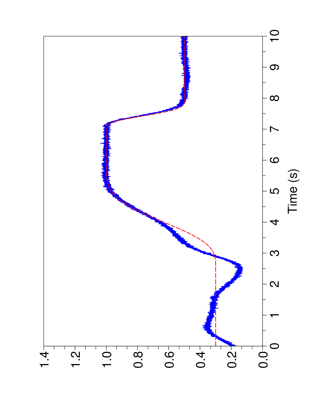
Figure 15: $y^{\star}(t)$ (- -) and $y(t)$ (–) with fault accommodation

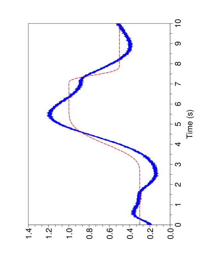
Figure 16: $y^{\star}(t)$ (- -) and $y(t)$ (–) without fault accommodation

7 Perturbation attenuation

7.0.1 Linear case

Suppose we are given a linear perturbed second order system

$$\ddot{y}(t)+y(t)=u(t)-z(t)+C\mathbf{1}(t-t_{I})$$ (21)

where

• $z(t)$ is an unknown perturbation input,

• $\mathbf{1}(t)$ is the Heaviside step function, i.e.,

  $$\mathbf{1}(t)=\left\{\begin{array}[]{l}0\quad\mbox{\rm if}\quad t<0\\ 1\quad\mbox{\rm if}\quad t\geq 0\end{array}\right.$$

• $C$ is an unknown constant and thus $C\mathbf{1}(t-t_{I})$ is a constant bias, of unknown amplitude, starting at time $t_{I}\geq 0$.

Remark 7.1.

The difference $C\mathbf{1}(t-t_{I})-z(t)$ is a rationally determinable variable according to Section 2.7.3.

The estimate $z_{e}(t)$ of $z(t)$ is given up to a piecewise constant error by

$$z_{e}(t)=-\ddot{y}_{e}(t)-y_{e}(t)+u(t)$$

where $y_{e}(t)$ and $\ddot{y}_{e}(t)$ are the on-line estimated values of $y(t)$ and $\ddot{y}(t)$. We design a generalized-proportional-integral (GPI) regulator, in order to track asymptotically a given output reference trajectory $y^{\star}(t)$, i.e.,

$$u(t)=y_{e}(t)+z_{e}(t)+{\ddot{y}}^{\star}(t)+\mathcal{G}\star(y_{e}(t)-y^{\ast}(t))$$ (22)

where

• $\mathcal{G}$ is defined via its rational transfer function $\frac{c_{2}s^{2}+c_{1}s+c_{0}}{s(s+c_{3})}$

• $s^{4}+c_{3}s^{3}+c_{2}s^{2}+c_{1}s+c_{0}$ is the characteristic polynomial of the unperturbed closed-loop system. The coefficients $c_{0},c_{1},c_{2},c_{3}$ are chosen so that the imaginary parts of its roots are strictly negative.

Like usual proportional-integral-derivative (PID) regulators, this controller is robust with respect to un-modeled piecewise constant errors

The computer simulations were performed with

$$z(t)=\frac{10t^{3}\sin(2t)}{1+t^{2}+t^{3}}$$

The unknown constant perturbation suddenly appears at time $t_{I}=4$ with a permanent value $C=1.25$. The coefficients of the characteristic polynomial were forced to be those of the desired polynomial $P_{d}(s)=(s^{2}+2\zeta\omega_{n}s+\omega_{n}^{2})^{2}$, with $\zeta=0.81$, $\omega_{n}=4$. We have set $y^{\star}(t)=\sin\omega t$, $\omega=2.5$[rad/s].

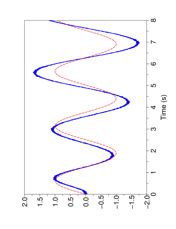
Figure 17: $y^{\star}(t)$ (- -) and $y(t)$ (–) without perturbation attenuation

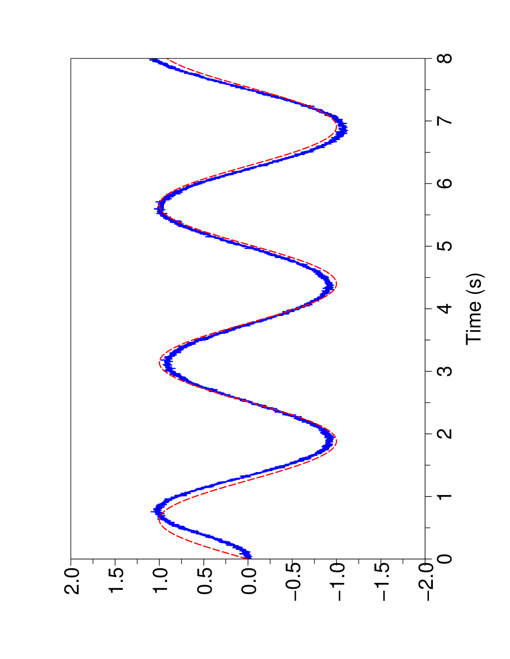
Figure 18: $y^{\star}(t)$ (- -) and $y(t)$ (–) with perturbation attenuation

Figure 17 (resp. 18) shows the reference signal $y^{\star}(t)$ and the output signal $y(t)$ without estimating $z_{e}(t)$ (resp. with the estimate $z_{e}(t)$). We added in the simulations of Figure 18 a Gaussian white noise $N(0;0.025)$ to the measurement $y(t)$. The results are quite remarkable.

Remark 7.2.

The same technique yields an efficient solution to fault tolerant linear control, which completes Fliess, Join & Sira-Ramírez (2004). Just think at $z(t)$ as a fault variable.

7.0.2 Non-linear extension

Replace the term $y(t)$ in system (21) by the product $y(t){\dot{y}}(t)$:

$$\ddot{y}(t)+y(t){\dot{y}}(t)=u(t)-z(t)+C\mathbf{1}(t-t_{I})$$ (23)

The perturbations $z(t)$ and $C\mathbf{1}(t-t_{I})$ are the same as above. The estimate $z_{e}(t)$ of $z(t)$ up to a piecewise constant is given by

$$z_{e}(t)=-{\ddot{y}}_{e}(t)-y_{e}{\dot{y}}_{e}(t)+u(t)$$

where $y_{e}(t)$, ${\dot{y}}_{e}(t)$ and ${\ddot{y}}_{e}(t)$ are the estimates of $y(t)$, ${\dot{y}}(t)$ and ${\ddot{y}}(t)$. The feedback law (22) becomes

$$u=y_{e}(t)\dot{y}_{e}(t)+z_{e}(t)+{\ddot{y}}^{\star}(t)+\mathcal{G}\star(y_{e}(t)-y^{\ast}(t))$$ (24)

Remark 7.3.

Rewrite system (23) via the following state variable representation

$$\left\{\begin{array}[]{l}{\dot{x}}_{1}(t)=x_{2}(t)\\ {\dot{x}}_{2}(t)=-x_{1}(t)x_{2}(t)+u(t)-z(t)+C\mathbf{1}(t-t_{I})\\ y(t)=x_{1}(t)\end{array}\right.$$

Applying the feedback law (24) amounts possessing good estimates of the two state variables.

Figures 19 and 20 depict the computer simulations with the same numerical conditions as before. The results are again excellent.

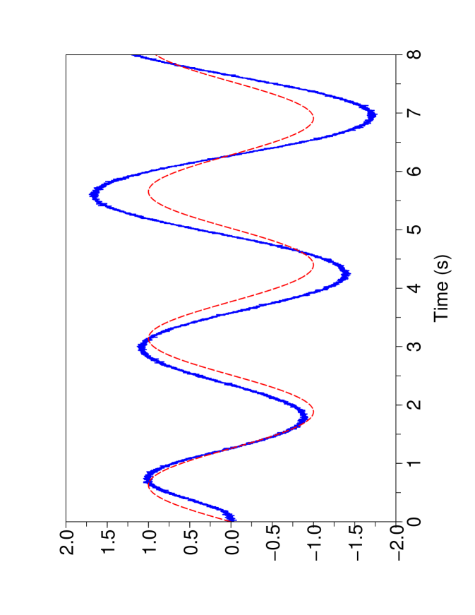
Figure 19: $y^{\star}(t)$ (- -) and $y(t)$ (–) without perturbation attenuation

Figure 20: $y^{\star}(t)$ (- -) and $y(t)$ (–) with perturbation attenuation.

8 Conclusion

We have proposed a new approach to non-linear estimation, which is not of asymptotic nature and does not necessitate any statistical knowledge of the corrupting noises. Promising results have already been obtained, which will be supplemented in a near future by other theoretical advances (see, e.g., Barbot, Fliess & Floquet (2007) on observers with unknown inputs) and several concrete case-studies (see already García-Rodríguez & Sira-Ramírez (2005); Nöthen (2007)). Further numerical improvements will also be investigated (see already Mboup, Join & Fliess (2007)).

ACKNOWLEDGMENT Two authors (MF & CJ) wish to thank M. Mboup for a most fruitful cooperation on numerical differentiation.

References

- Aström, Blanke, Isidori, Schaufelberger & Sanz (2001) Aström, K.J., Albertos, P., Blanke, M., Isidori, A., Schaufelberger, W., and Sanz, R. (2001) Control of Complex Systems, Springer.
- Atiyah & Macdonald (1969) Atiyah, M.F., and Macdonald, I.G. (1969) Introduction to Commutative Algebra, Addison-Wesley.
- Barbot, Fliess & Floquet (2007) Barbot, J.P., Fliess, M., and Floquet, T. (2007) ‘An algebraic framework for the design of nonlinear observers with unknown inputs’, Proc. IEEE Conf. Decision Control, New Orleans (available at http://hal.inria.fr/inria-00172366).
- Blanke, Kinnaert, Lunze & Staroswiecki (2003) Blanke, M., Kinnaert, M., Lunze, J., and Staroswiecki, M. (2003) Diagnosis and Fault-Tolerant Control, Springer.
- Bourlès (2006) Bourlès, H. (2006) Systèmes linéaires : de la modélisation à la commande, Hermès.
- Braci & Diop (2001) Braci, M., and Diop, S. (2001) ‘On numerical differentiation algorithms for nonlinear estimation’, Proc. IEEE Conf. Decision Control, Maui, Hawaii.
- Busvelle & Gauthier (2003) Busvelle, E., and Gauthier, J.P. (2003) ‘On determining unknown functions in differential systems, with an application to biological reactors’, ESAIM Control Optimis. Calculus Variat., Vol. 9, pp. 509-552.
- Chambert-Loir (2005) Chambert-Loir, A. (2005) Algèbre corporelle, Éditions École Polytechnique. English translation (2005): A Field Guide to Algebra, Springer.
- Chen & Patton (1999) Chen, J., and Patton, R. (1999). Robust Model-Based Fault Diagnosis for Dynamic Systems, Kluwer.
- Chetverikov (2004) Chetverikov, V.N. (2004) ‘A nonlinear Spencer complex for the group of invertible differential operators and its applications’, Acta Appl. Math., Vol. 83, pp. 1-23.
- Chitour (2002) Chitour, Y. (2002) ‘Time-varying high-gain observers for numerical differentiation’, IEEE Trans. Automat. Control, Vol. 47, pp. 1565-1569.
- Conte, Moog & Perdon (1999) Conte, G., Moog, C.H., and Perdon, A.M. (1999) Nonlinear Control Systems – An Algebraic Setting, Lect. Notes Control Informat. Sci., Vol. 242, Springer.
- Dabroom & Khalil (1999) Dabroom, A.M., and Khalil, H.K. (1999) ‘Discrete-time implementation of high-gain observers for numerical differentiation’, Int. J. Control, Vol. 72, pp. 1523-1537.
- Delaleau (2002) Delaleau, E. (2002) ‘Algèbre différentielle’, in J.P. Richard (Ed.): Mathématiques pour les Systèmes Dynamiques, Vol. 2, chap. 6, pp. 245-268, Hermès.
- Delaleau & Pereira da Silva (1998a) Delaleau, E., and Pereira da Silva, P.S. (1998a) ‘Filtrations in feedback synthesis: Part I - systems and feedbacks’, Forum Math., Vol. 10, pp. 147-174.
- Delaleau & Pereira da Silva (1998b) Delaleau, E., and Pereira da Silva, P.S. (1998b) ‘Filtrations in feedback synthesis - Part II: input-output decoupling and disturbance decoupling’, Forum Math., Vol. 10, pp. 259-276.
- Delaleau & Respondek (1995) Delaleau, E., and Respondek, W. (1995) ‘Lowering the orders of derivatives of control in generalized state space systems’ J. Math. Systems Estim. Control, Vol. 5, pp. 1-27.
- Delaleau & Rudolph (1998) Delaleau, E., and Rudolph, J. (1998) ‘Control of flat systems by quasi-static feedback of generalized states’, Int. J. Control, Vol. 71, pp. 745-765.
- Diop (1991) Diop, S. (1991) ‘Elimination in control theory’, Math. Control Signals Systems, Vol. 4, pp. 17-32.
- Diop (1992) Diop, S. (1992) ‘Differential algebraic decision methods, and some applications to system theory’, Theoret. Comput. Sci., Vol. 98, pp. 137-161
- Diop (2002) Diop, S. (2002) ‘From the geometry to the algebra of nonlinear observability’, in A. Anzaldo-Meneses, B. Bonnard, J.P. Gauthier, and F. Monroy-Perez (Eds.): Contemporary Trends in Nonlinear Geometric Control Theory and its Applications, pp. 305-345, World Scientific.
- Diop & Fliess (1991a) Diop, S., and Fliess, M. (1991a) ‘On nonlinear observability’, Proc. Europ. Control Conf., Hermès, pp. 152-157.
- Diop & Fliess (1991b) Diop S., and Fliess, M. (1991b) ‘Nonlinear observability, identifiability and persistent trajectories’, Proc. IEEE Conf. Decision Control, Brighton, pp. 714-719.
- Diop, Fromion & Grizzle (2001) Diop, S., Fromion, V., and Grizzle, J.W. (2001) ‘A global exponential observer based on numerical differentiation’, Proc. IEEE Conf. Decision Control, Orlando.
- Diop, Grizzle & Chaplais (2000) Diop, S., Grizzle, J.W., and Chaplais, F. (2000) ‘On numerical differentiation for nonlinear estimation’, Proc. IEEE Conf. Decision Control, Sidney.
- Diop, Grizzle, Moraal & Stefanopoulou (1994) Diop, S., Grizzle, J.W., Moraal, P.E., and Stefanopoulou, A. (1994) ‘Interpolation and numerical differentiation for observer design’, Proc. Amer. Control Conf., Baltimore, pp. 1329-1333.
- Duncan, Madl & Pasik-Duncan (1996) Duncan, T.E., Mandl, P., and Pasik-Duncan, B. (1996) ‘Numerical differentiation and parameter estimation in higher-order linear stochastic systems’, IEEE Trans. Automat. Control, Vol. 41, pp. 522-532.
- Eisenbud (1995) Eisenbud, D. (1995) Commutative Algebra with a View Toward Algebraic Geometry, Springer.
- Fan & Arcak (2003) Fan, X., and Arcak, M. (2003) ‘Observer design for systems with multivariable monotone nonlinearities’, Systems Control Lett., Vol. 50, pp. 319-330.
- Fliess (1989) Fliess, M. (1989) ‘Automatique et corps différentiels’, Forum Math., Vol. 1, pp. 227-238.
- Fliess (1990) Fliess, M. (1990) ‘Controller canonical forms for linear and nonlinear dynamics’, IEEE Trans. Automat. Control, Vol. 33, pp. 994-1001.
- Fliess (1994) Fliess, M. (1994) ‘Une inteprétation algébrique de la transformation de Laplace et des matrices de transfert’, Linear Algebra Appl., Vol. 203-204, pp. 429-442.
- Fliess (2000) Fliess, M. (2000) ‘Variations sur la notion de contrôlabilité’, Journée Soc. Math. France, Paris (available at http://hal.inria.fr/inria-00001042).
- Fliess (2006) Fliess, M. (2006) ‘Analyse non standard du bruit’, C.R. Acad. Sci. Paris Ser. I, Vol. 342, pp. 797-802.
- Fliess & Hasler (1990) Fliess, M., and Hasler M. (1990) ‘Questioning the classical state space description via circuit examples’, in M. Kashoek, J. van Schuppen and A. Ran (Eds.): Realization and Modelling in System Theory, MTNS-89, Vol 1, pp. 1-12, Birkhäuser.
- Fliess, Join, Mboup & Sedoglavic (2005) Fliess, M., Join, C., Mboup, M., and Sedoglavic, A. (2005) ‘Estimation des dérivées d’un signal multidimensionnel avec applications aux images et aux vidéos’, Actes Coll. GRETSI, Louvain-la-Neuve (available at http//hal.inria.fr/inria-00001116).
- Fliess, Join, Mboup & Sira-Ramírez (2004) Fliess, M., Join, C., Mboup, M., and Sira-Ramírez, H. (2004) ‘Compression différentielle de transitoires bruités’, C.R. Acad. Sci. Paris Ser. I, Vol. 339, pp. 821-826.
- Fliess, Join, Mboup & Sira-Ramírez (2005) Fliess, M., Join, C., Mboup, M., and Sira-Ramírez, H. (2005) ‘Analyse et représentation de signaux transitoires : application à la compression, au débruitage et à la détection de ruptures’, Actes Coll. GRETSI, Louvain-la-Neuve (available at http://hal.inria.fr/inria-00001115).
- Fliess, Join & Sira-Ramírez (2004) Fliess, M., Join, C., and Sira-Ramírez, H. (2004) ‘Robust residual generation for linear fault diagnosis: an algebraic setting with examples’, Int. J. Control, Vol. 77, pp. 1223-1242.
- Fliess, Join & Sira-Ramírez (2005) Fliess, M., Join, C., and Sira-Ramírez, H. (2005) ‘Closed-loop fault-tolerant control for uncertain nonlinear systems’, in T. Meurer, K. Graichen, E.D. Gilles (Eds.): Control and Observer Design for Nonlinear Finite and Infinite Dimensional Systems, Lect. Notes Control Informat. Sci., vol. 322, pp. 217-233, Springer.
- Fliess, Lévine, Martin & Rouchon (1995) Fliess, M., Lévine, J., Martin, P., and Rouchon, P. (1995) ‘Flatness and defect of non-linear systems: introductory theory and examples’, Int. J. Control, Vol. 61, pp. 1327-1361.
- Fliess, Lévine, Martin & Rouchon (1997) Fliess, M., Lévine, J., Martin, P., and Rouchon, P. (1997) ‘Deux applications de la géometrie locale des diffiétés’, Ann. Inst. H. Poincaré Phys., Vol. 66, pp. 275-292.
- Fliess, Lévine, Martin & Rouchon (1999) Fliess, M., Lévine, J., Martin, P., and Rouchon, P. (1999) ‘A Lie-Bäcklund approach to equivalence and flatness of nonlinear systems’, IEEE Trans. Automat. Control, Vol. 44, pp. 922-937.
- Fliess, Lévine & Rouchon (1993) Fliess, M., Lévine, J., and Rouchon, P. (1993) ‘Generalized state variable representation for a simplified crane description’, Int. J. Control, Vol. 58, pp. 277-283.
- Fliess, Marquez, Delaleau & Sira-Ramírez (2002) Fliess, M., Marquez, R., Delaleau, E., and Sira-Ramírez, H. (2002) ‘Correcteurs proportionnels-intégraux généralisés’, ESAIM Control Optim. Calc. Variat., Vol. 7, pp. 23-41.
- Fliess & Rudolph (1997) Fliess, M., and Rudolph, J. (1997) ‘Corps de Hardy et observateurs asymptotiques Iocaux pour systèmes différentiellement plats’, C.R. Acad. Sci. Paris Ser. II, Vol. 324, pp. 513-519.
- Fliess & Sira-Ramírez (2003) Fliess, M., and Sira-Ramírez, H. (2003) ‘An algebraic framework for linear identification’, ESAIM Control Optim. Calc. Variat., Vol. 9, pp. 151-168.
- Fliess & Sira-Ramírez (2004a) Fliess, M., and Sira-Ramírez, H. (2004a) ‘Reconstructeurs d’état’, C.R. Acad. Sci. Paris Ser. I, Vol. 338, pp. 91-96.
- Fliess & Sira-Ramírez (2004b) Fliess, M., and Sira-Ramírez, H. (2004b) ‘Control via state estimations of some nonlinear systems’, Proc. Symp. Nonlinear Control Systems (NOLCOS 2004), Stuttgart (available at http//hal.inria.fr/inria-00001096).
- Fliess & Sira-Ramírez (2007) Fliess, M., and Sira-Ramírez, H. (2007) ‘Closed-loop parametric identification for continuous-time linear systems’, in H. Garnier & L. Wang (Eds.): Continuous-Time Model Identification from Sampled Data, Springer (available at http://hal.inria.fr/inria-00114958).
- García-Rodríguez & Sira-Ramírez (2005) García-Rodríguez, C., and Sira-Ramírez, H. (2005) ‘Trajectory tracking via algebraic methods for state estimation’, in Proc. IEEE Int. Congress Innovation Technological Develop., Cuernavaca, Mexico.
- Gauthier & Kupka (2001) Gauthier, J.-P, and Kupka, I.A.K. (2001) Deterministic Observation Theory and Applications, Cambridge University Press.
- Gertler (1998) Gertler, J.J. (1998) Fault Detection and Diagnosis in Engineering Systems, Marcel Dekker.
- Glad (2006) Glad, S.T. (2006) ‘Using differential algebra to determine the structure of control systems’, in B. Hanzon and M. Hazewinkel (Eds.): Constructive Algebra and Systems Theory, Royal Netherlands Academy of Arts and Sciences, pp. 323-340.
- Hartshorne (1977) Hartshorne, R. (1977) Algebraic Geometry, Springer.
- Hermann & Krener (1977) Hermann, R., and Krener, A.J. (1977) ‘Nonlinear controllability and observability’, IEEE Trans. Automat. Control, Vol. 22, pp. 728-740.
- Ibrir (2003) Ibrir, S. (2003) ‘Online exact differentiation and notion of asymptotic algebraic observers’, IEEE Trans. Automat. Control, Vol. 48, pp. 2055-2060.
- Ibrir (2004) Ibrir, S. (2004) ‘Linear time-derivatives trackers’, Automatica, Vol. 40, pp. 397-405.
- Ibrir & Diop (2004) Ibrir, S., and Diop, S. (2004) ‘A numerical procedure for filtering and efficient high-order signal differentiation’, Int. J. Appl. Math. Comput. Sci., Vol. 14, pp. 201-208.
- Isidori (1995) Isidori, A. (1995) Nonlinear Control Systems, 3rd ed., Springer.
- Jaulin, Kiefer, Didrit & Walter (2001) Jaulin, L., Kieffer, M., Didrit, O., and Walter, E. (2001) Applied Interval Analysis, Springer.
- Johnson (1969) Johnson J. (1969) ‘Kähler differentials and differential algebra’, Annals Math. Vol. 89, pp. 92-98.
- Kelly, Ortega, Ailon & Loria (1994) Kelly, R., Ortega, R., Ailon, A., and Loria, A. (1994) ‘Global regulation of flexible joint robots using approximate differentiation’, IEEE Trans. Automat. Control, Vol. 39, pp. 1222-1224.
- Kolchin (1973) Kolchin, E.R. (1973) Differential Algebra and Algebraic Groups, Academic Press.
- Lamnabhi-Lagarrigue & Rouchon (2002a) Lamnabhi-Lagarrigue, F., and Rouchon P. (Eds.) (2002a) Systèmes non linéaires, Hermès.
- Lamnabhi-Lagarrigue & Rouchon (2002b) Lamnabhi-Lagarrigue, F., and Rouchon P. (Eds.) (2002b) Commandes non linéaires, Hermès.
- Levant (1998) Levant, A. (1998) ‘Robust exact differentiation via sliding mode technique’, Automatica, Vol. 34, pp. 379-384.
- Levant (2003) Levant, A. (2003) ‘Higher-order sliding modes, differentiation and output-feedback control’, Int. J. Cpntrol, Vol. 76, pp. 924-941.
- Levine (1996) Levine, W. (Ed.) (1996) The Control Systems Handbook, CRC Press.
- Ljung & Glad (1994) Ljung, L., and Glad, T. (1994) ‘On global identifiability for arbitrary model parametrizations’, Automatica, Vol. 30, pp. 265-276.
- Li, Chiasson, Bodson & Tolbert (2006) Li, M., Chiasson, J., Bodson, M., and Tolbert, L.M. (2006) ‘A differential-algebraic approach to speed estimation in an induction motor’, IEEE Trans. Automat. Control, Vol. 51, pp. 1172-1177.
- Mai, Join & Reger (2007) Mai, P., Join, C., and Reger, J. (2007) ‘Flatness-based fault tolerant control of a nonlinear MIMO system using algebraic derivative estimation’, Proc. IFAC Symp. System Structure Control (SSSC07), Foz do Iguaçu, Brazil.
- Martin & Rouchon (1994) Martin, P., and Rouchon, P. (1994) ‘Feedback linearization and driftless systems’, Math. Control Signal Syst., Vol. 7, pp. 235-254, 1994.
- Martin & Rouchon (1995) Martin, P., and Rouchon, P. (1995) ‘Any (controllable) driftless system with 3 inputs and 5 states is flat’, Systems Control Lett., Vol. 25, pp. 167-173.
- Martinez-Guerra & Diop (2004) Martinez-Guerre, R., and Diop, S. (2004) ‘Diagnosis of nonlinear systems using an unknown-input observer: an algebraic and differential approach’, IEE Proc. Control Theory Applications, Vol. 151, pp. 130-135.
- Martìnez-Guerra, González-Galan, Luviano-Juárez & Cruz-Victoria (2007) Martínez-Guerra, R., González-Galan, R., Luviano-Juárez, A., and Cruz-Victoria, J. (2007) ‘Diagnosis for a class of non-differentially flat and Liouvillian systems’, IMA J. Math. Control. Informat., Vol. 24.
- Mboup, Join & Fliess (2007) Mboup, M., Join, C., and Fliess, M. (2007) ‘A revised look at numerical differentiation with an application to nonlinear feedback control’, Proc. 15th Mediterrean Conf. Control Automation (MED’2007), Athens (available at http://hal.inria.fr/inria-00142588).
- McConnell & Robson (2000) McConnell J., Robson J. (2000) Noncommutative Noetherian Rings, American Mathematical Society.
- Menini, Zaccarian & Abdallah (2006) Menini, L., Zaccarian, C., and Abdallah, C.T. (Eds.) (2006) Current Trends in Nonlinear Systems and Control, Birkhäuser.
- Mikusinski (1983) Mikusinski, J. (1983) Operational Calculus, ed., Vol. 1, PWN & Pergamon.
- Mikusinski & Boehme (1987) Mikusinski, J., and Boehme, T. (1987) Operational Calculus, ed., Vol. 2, PWN & Pergamon.
- van Nieuwstadt, Rathinam & Murray (1998) van Nieuwstadt, M., Rathinam, M., and Murray, R.M. (1998) ‘Differential flatness and absolute equivalence of nonlinear control systems’, SIAM J. Control Optimiz., Vol. 36, pp. 1225-1239.
- Nijmeijer & Fossen (1999) Nijmeijer, H., and Fossen, T.I. (Eds.) (1999) New Directions in Nonlinear Observer Design, Lect. Notes Control Informat. Sci., Vol. 244, Springer.
- Nijmeijer & van der Schaft (1990) Nijmeijer, H., and van der Schaft, A.J. (1990) Nonlinear Dynamical Control Systems, Springer.
- Nöthen (2007) Nöthen, C. (2007) Beiträge zur Rekonstruktion nicht direkt gemessener Größen bei der Silizium-Einkristallzüchtung nach dem Czochralski-Verfahren, Diplomarbeit, Technische Universität Dresden.
- Ollivier (1990) Ollivier, F. (1990) Le problème de l’identifiabilité structurelle globale : approche théorique, méthodes effectives et bornes de complexité, Thèse, École Polytechnique, Palaiseau, France.
- Ollivier & Sedoglavic (2002) Ollivier, F., and Sedoglavic, A. (2002) ‘Algorithmes efficaces pour tester l’identifiabilité locale’, Actes Conf. Int. Francoph. Automatique (CIFA 2002), Nantes.
- Pomet (1997) Pomet, J.-B. (1997) ‘On dynamic feedback linearization of four-dimensional affine control systems with two inputs’, ESAIM Control Optimis. Calculus Variat., Vol. 2, pp. 151-230.
- Reger, Mai & Sira-Ramírez (2006) Reger, J., Mai, P., and Sira Ramírez, H. (2006) ‘Robust algebraic state estimation of chaotic systems’, Proc. IEEE 2006 CCA/CACSD/ISIC, Munich.
- Ritt (1950) Ritt, J.F. (1950) Differential Algebra, American Mathematical Society.
- Rudolph (2003) Rudolph, J. (2003) Beiträge zur flacheitsbasierten Folgeregelung linearer und nichtlinearer Syteme endlicher und undendlicher Dimension, Shaker Verlag.
- Rudolph & Delaleau (1998) Rudolph, J., and Delaleau, E. (1998) ‘Some examples and remarks on quasi-static feedback of generalized states’, Automatica, Vol. 34, pp. 993-999.
- Saccomani, Audoly & D’Angio (2003) Saccomania, M.P., Audoly, S., D’Angio, L. (2003) ‘Parameter identifiability of nonlinear systems: the role of initial conditions’, Automatica, Vol. 39, pp. 619-632.
- Sastry (1999) Sastry, S. (1999) Nonlinear Systems, Springer.
- Schweppe (1973) Schweppe, F.C. (1973) Uncertain Dynamic Systems, Prentice Hall.
- Sedoglavic (2002) Sedoglavic, A. (2002) ‘A probabilistic algorithm to test local algebraic observability in polynomial time’, J. Symbolic Computation, Vol. 33, pp. 735-755.
- Sira-Ramírez & Agrawal (2004) Sira-Ramírez, H., and Agrawal, S.K. (2004) Differentially Flat Systems, Marcel Dekker.
- Sira-Ramírez & Fliess (2006) Sira-Ramírez, H., and Fliess, M. (2006) ‘An algebraic state estimation approach for the recovery of chaotically encrypted messages’, Int. J. Bifurcation Chaos, Vol. 16, pp. 295-309.
- Slotine (1991) Slotine, J.J. (1991) Applied Nonlinear Control, Prentice Hall.
- Smolin (2006) Smolin, L. (2006) The Trouble with Physics - The Rise of String Theory, the Fall of Science, and What Comes Next, Houghton Mifflin.
- Sontag (1998) Sontag, E.D. (1998) Mathematical Control Theory, 2nd ed., Springer.
- Staroswiecki & Comtet-Varga (2001) Staroswiecki, M., and Comtet-Varga, G. (2001) ‘Analytic redundancy for fault detection and isolation in algebraic dynamic system’, Automatica, Vol. 37, pp. 687 699.
- Su, Zheng, Mueller & Duan (2006) Su, Y.X., Zheng, C.H., Mueller, P.C., and Duan, B.Y. (2006) ‘A simple improved velocity estimation for low-speed regions based on position measurements only’, IEEE Trans. Control Systems Technology, Vol. 14, pp. 937-942.
- Vachtsevanos, Lewis, Roemer, Hess & Wu (2006) Vachtsevanos, G., Lewis, F.L., Roemer, M., Hess, A., and Wu, B. (2006) Intelligent Fault Diagnosis and Prognosis for Engineering Systems, Wiley.
- Yosida (1984) Yosida, K. (1984) Operational Calculus: A Theory of Hyperfunctions (translated from the Japanese), Springer.
- Zhang, Basseville & Benveniste (1998) Zhang, Q., Basseville, M., and Benveniste, A. (1998) ‘Fault detection and isolation in nonlinear dynamic systems: a combined input-output and local approach’, Automatica, Vol. 34, pp. 1359-1373.
- Zinober & Owens (2002) Zinober, A., and Owens, D.H. (Eds.) (2002) Nonlinear and Adaptive Control, Lect. Notes Control Informat. Sci., Vol. 281, Springer.