Unzipping of two random heteropolymers: Ground state energy and finite size effects

Abstract

We have analyzed the dependence of average ground state energy per monomer, $e$, of the complex of two random heteropolymers with quenched sequences, on chain length, $n$, in the ensemble of chains with uniform distribution of primary sequences. Every chain monomer is randomly and independently chosen with the uniform probability distribution $p=1/c$ from a set of $c$ different types A, B, C, D, …. Monomers of the first chain could form saturating reversible bonds with monomers of the second chain. The bonds between similar monomer types (like A–A, B–B, C–C, etc.) have the attraction energy $u$, while the bonds between different monomer types (like A–B, A–D, B–D, etc.) have the attraction energy $v$. The main attention is paid to the computation of the normalized free energy $e(n)$ for intermediate chain lengths, $n$, and different ratios $a=\frac{v}{u}$ at sufficiently low temperatures when the entropic contribution of the loop formation is negligible compared to direct energetic interactions between chain monomers and the partition function of the chains is dominated by the ground state. The performed analysis allows one to derive the force, $f$, which is necessary to apply for unzipping of two random heteropolymer chains of equal lengths whose ends are separated by the distance $x$, averaged over all equally distributed primary structures at low temperatures for fixed values $a$ and $c$.

PACS numbers: 02.50.-r, 05.40.-a, 87.10.-e, 87.15.Cc

I Introduction

Recent progress in nanotechnology has offered a possibility of single–molecular experiments. The corresponding technique allows one to investigate many physico–chemical and biological properties of individual molecules. One of the modern biophysical key experiments deals with the mechanical unzipping of individual double–stranded DNA macromolecule under the action of external force applied to the ends of strands. This question has been analyzed theoretically in a number of important contributions nel_lub1 ; bhat1 ; seb ; mon ; bhat2 ; nel_lub2 ; cule ; tang ; singh . Some of them are devoted to the consideration of unzipping transition in an effective homopolymer chain, the other pay attention to the heterogeneity of primary sequence of complimentary strands constituting the DNA molecule.

In our work we address a problem of unzipping of a complex of two random heteropolymers of finite lengths at sufficiently low temperatures when the partition function is dominated by the ground state. We demonstrate that this problem can be mapped to the problem of alignment of two random sequences with the general ”cost function” which takes into account the weights of perfect matches, mismatches and gaps (all necessary definitions are introduced below). Using this bijection we are able to compute the external work necessary to unzip the complex of two random heteropolymers, averaged over the uniform distribution of all possible primary sequences of heteropolymers. Our consideration allows also to conjecture the scaling corrections to the leading behavior of the force fluctuations due to the finiteness of the lengths of heteropolymer chains.

The paper is organized as follows. In Section II we define a model under consideration and introduce the basic notations. In Section III we consider unzipping of two random heteropolymers from the point of view of the search of Longest Common Subsequence (LcS) of two random sequences. The expectation of the LCS energy is considered in Section IV. In Conclusion we give the qualitative explanation of our main results and derive a force, which is necessary to apply to the chain ends to unzip two random heteropolymer chains at low temperatures.

II The model

Consider two random heteropolymer chains of lengths $L_{1}=m\ell$ and $L_{2}=n\ell$ correspondingly. In what follows we shall measure the lengths of the chains in number of monomers, $m$ and $n$, supposing that the size of an elementary unit, $\ell$, is equal to 1. Every monomer can be randomly and independently chosen with the uniform probability distribution $p=\frac{1}{c}$ from a set of $c$ different types A, B, C, D, … . Monomers of the first chain could form saturating reversible bonds with monomers of the second chain. The term ”saturating” means that any monomer can form a bond with at most one monomer of the other chain. The bonds between similar types (like A–A, B–B, C–C, etc.) have the attraction energy $u$ and are called below ”matches”, while the bonds between different types (like A–B, A–D, B–D, etc.) have the attraction energy $v$ and are called ”mismatches”. Some parts of the chains could form loops hence contributing to the entropic part of the free energy of the system. Schematically a particular configuration of the system under consideration for $c=2$ is shown in Fig.1.

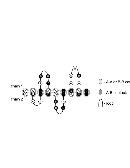
Figure 1: Schematic picture of a complex of two random heteropolymer chains.

Our aim is to compute the free energy of the described model at sufficiently low temperatures when the entropic contribution of the loop formation is negligible compared to the energetic part of the direct interactions between chain monomers.

Consider now the partition function of such a complex $G_{m,n}$ which is the sum over all possible arrangements of bonds. Since we are interested in the low–temperature behavior of $G_{m,n}$, we neglect the entropic contribution of the loop weights which allows to write $G_{m,n}$ recursively in terms of the partition functions of individual chains $g(n)$:

$$\left\{\begin{array}[]{l}\displaystyle G_{m,n}=g(m)g(n)+\sum_{i,j=1}^{m,n}\beta_{i,j}\,G_{i-1,j-1}g(m-i)g(n-j)\vskip 6.0pt plus 2.0pt minus 2.0pt\\ G_{m,0}=g(m);\;\;G_{0,n}=g(n);\;\;G_{0,0}=1\end{array}\right.$$ (1)

The meaning of the equation (1) is as follows. Starting from, say, the left ends of the chains shown in Fig.1 we find the first actually existing contact between the monomers $i$ (of the first chain) and $j$ (of the second chain) and sum over all possible arrangements of this first contact. The first term ”1” in (1) means that we have not found any contact at all. The entries $\beta_{i,j}$ ($1\leq i\leq m,\;1\leq j\leq n$) are the statistical weights of the bonds which are encoded in a contact map $\{\beta\}$:

$$\beta_{m,n}=\begin{cases}\beta^{+}\equiv e^{u/T}&\mbox{if monomers $i$ and $j$ match}\\ \beta^{-}\equiv e^{v/T}&\mbox{if monomers $i$ and $j$ do not match}\end{cases}$$ (2)

For a system of two heteropolymer chains depicted in Fig.1 the contact map $\{\beta\}$ is shown in Fig.2.

Generally speaking, if one allows for loop formation within a single chain, the partition functions of individual chains $g(n)$ satisfy, in turn, recurrent equation deGennes; Erukh ; Mueller

$$g(n)=1+\sum_{i=1}^{n-1}\sum_{j=i+1}^{n}\beta^{\prime}_{i,j}g(j-i-1)g(n-j);\;\;g(0)=1$$ (3)

where $\beta^{\prime}_{i,j}$ are the constants of self-association, which are, similarly to $\beta_{m,n}$, random variables encoded by some contact map. However, for the sake of simplicity, we assume in this paper that there is no self-association in the systems under discussion, and thus

$$\beta^{\prime}\equiv 0;\;\;g(n)\equiv 1$$ (4)

This simplification is, in fact, rather significant from the mathematical point of view since we replace the quadratic set of equations (1), (3) with the linear set (1), (3). However, we expect the intrachain association to be effectively suppressed due to the finite flexibility of the single chains, and, therefore, the typical values of $\beta^{\prime}$ to be much less then the typical values of $\beta$. We expect thus the interchain association to give just some minor corrections to the results obtained below.

The case of non-zero $\beta^{\prime}$s was thoroughly investigated recently Bund2 ; Neher ; TN2 in a set-up when the interactions in the system are predetermined instead of random and we refer the reader to these papers for more detail.

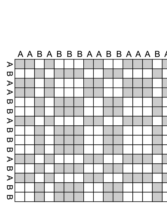
Figure 2: Contact map $\{\beta\}$ corresponding to the complex of two random heteropolymer chains shown in Fig.1.

III Unzipping of two random heteropolymers and search of longest common subsequence (LCS) of two random sequences

III.1 Heteropolymer ground state energy: local recursive construction

The straightforward computation shows that the partition function $G_{m,n}$ obeys the following exact local recursion

$$G_{m,n}=G_{m-1,n}+G_{m,n-1}+(\beta_{m,n}-1)\,G_{m-1,n-1}$$ (5)

Note that if $\beta_{i,j}=2$ for all $1\leq i\leq m$ and $1\leq j\leq n$, the recursion relation (5) generates the so-called Delannoy numbers delannoy .

Represent now the partition function $G_{m,n}$ in the following way

$$G_{m,n}=e^{F_{m,n}/T}$$ (6)

where $-F_{n,m}$ has the sense of the free energy and $T$ stands for the temperature of the complex of two heterogeneous chains of lengths $m$ and $n$. Considering the $T\to 0$ limit, we get

$$F_{m,n}=\lim_{T\to 0}T\ln\Big{(}e^{F_{m-1,n}/T}+e^{F_{m,n-1}/T}+(\beta_{m,n}-1)\,e^{F_{m-1,n-1}/T}\Big{)}$$ (7)

which can be regarded as the equation for the ground state energy of a chain. The expression (7) can be rewritten in a symbolic form

$$F_{m,n}=\max\left[F_{m-1,n},\,F_{m,n-1},\,F_{m-1,n-1}+\eta_{m,n}\right]$$ (8)

where

$$\eta_{m,n}=T\ln(\beta_{m,n}-1)=\begin{cases}\eta^{+}=T\ln(e^{u/T}-1)&\mbox{in case of match}\\ \eta^{-}=T\ln(e^{v/T}-1)&\mbox{in case of mismatch}\end{cases}$$ (9)

Taking $\eta^{+}$ as the unit of the energy, we can rewrite (8) as follows

$$\tilde{F}_{m,n}=\max\left[\tilde{F}_{m-1,n},\,\tilde{F}_{m,n-1},\,\tilde{F}_{m-1,n-1}+\tilde{\eta}_{m,n}\right]$$ (10)

where

$$\tilde{\eta}_{m,n}=\begin{cases}1&\mbox{in case of match}\\ \displaystyle a=\frac{\eta^{-}}{\eta^{+}}&\mbox{in case of mismatch}\end{cases}$$ (11)

In the low–temperature limit the parameter $a$ has simple expression in terms of coupling constants $u$ and $v$:

$$a=\frac{\eta^{-}}{\eta^{+}}=\left.\frac{\ln(e^{v/T}-1)}{\ln(e^{u/T}-1)}\right|_{T\to 0}=\frac{v}{u}$$ (12)

Finally, the initial conditions for $\tilde{F}_{m,n}$ transform due to the second of equations (1) into

$$\tilde{F}_{0,n}=\tilde{F}_{n,0}=\tilde{F}_{0,0}=0$$ (13)

III.2 Matching with gaps: the cost function

In Eqs.(8)–(13) we can recognize the recursive algorithm Gusfield ; Monvel for the determination of the length $F_{m,n}$ of the Longest Common Subsequence (LCS) of two arbitrary sequences of lengths $m$ and $n$. It is easy to see that the search of $F_{m,n}$ can be completed in polynomial time $\sim O(mn)$.

Recall that the problem of finding the LCS in a pair of sequences drawn from alphabet of $c$ letters is formulated as follows. Consider two sequences $\alpha=\{\alpha_{1},\alpha_{2},\dots,\alpha_{m}\}$ (of length $m$) and $\beta=\{\beta_{1},\beta_{2},\dots,\beta_{n}\}$ (of length $n$). For example, let $\alpha$ and $\beta$ be two random sequences of $c=4$ base pairs A, C, G, T of a DNA molecule, e.g., $\alpha=\{\rm A,C,G,C,T,A,C\}$ with $m=6$ and $\beta=\{\rm C,T,G,A,C\}$ with $n=5$. Any subsequence of $\alpha$ (or $\beta$) is an ordered sublist of $\alpha$ (and of $\beta$) entries which need not to be consecutive, e.g, it could be $\{\rm C,G,T,C\}$, but not $\{\rm T,G,C\}$. A common subsequence of two sequences $\alpha$ and $\beta$ is a subsequence of both of them. For example, the subsequence $\{\rm C,G,A,C\}$ is a common subsequence of both $\alpha$ and $\beta$. There are many possible common subsequences of a pair of initial sequences. The aim of the LCS problem is to find the longest of them. This problem and its variants have been widely studied in biology NW ; SW ; WGA ; AGMML , computer science SK ; AG ; WF ; Gusfield , probability theory CS ; Deken ; Steele ; DP ; Alex ; KLM and more recently in statistical physics ZM ; Hwa ; Monvel . A particularly important application of the LCS problem is to quantify the closeness between two DNA sequences. In evolutionary biology, the genes responsible for building specific proteins evolve with time and by finding the LCS of similar genes in different species, one can learn what has been conserved in time. Also, when a new DNA molecule is sequenced in vitro, it is important to know whether it is really new or it is similar to already existing molecules. This is achieved quantitatively by measuring the LCS of the new molecule with other ones available from database.

In the simplest version of the LCS problem only the number of perfect matches is taken into account, i.e. there is no difference between mismatches and gaps. One can, however, easily construct a generalized model where this difference comes into play. Let us introduce the general ”cost function”, ${\cal S}$, having a meaning of an energy (see, for example Hwa97 ; HWA2 for details)

$${\cal S}=N_{\rm match}+\mu\,N_{\rm mis}+\delta\,N_{\rm gap}$$ (14)

In (14) $N_{\rm match}$, $N_{\rm mis}$ and $N_{\rm gap}$ are correspondingly the numbers of matches, mismatches and gaps in a given pair of sequences—see Fig.3, and $\mu$ and $\delta$ are respectively the energies of mismatches and gaps. Without the loss of generality the energy of matches can be always set to 1. Besides (14) we have an obvious conservation law

$$n+m=2N_{\rm match}+2N_{\rm mis}+N_{\rm gap}$$ (15)

which allows one to exclude $N_{\rm gap}$ from (14) and rewrite this expression as follows:

$${\cal S}=N_{\rm match}+\mu N_{\rm mis}+\delta(n+m-2N_{\rm match}-2N_{\rm mis})=(1-2\delta)N_{\rm match}+(\mu-2\delta)N_{\rm mis}+{\rm const}$$ (16)

In (16) the irrelevant constant $\delta(n+m)$ can be dropped out.

Now we can adopt $(1-2\delta)$ as a unit of energy. Finally we arrive at the following expression

$$\tilde{\cal S}=N_{\rm match}+\gamma N_{\rm mis}$$ (17)

where

$$\gamma=\frac{\mu-2\delta}{1-2\delta},$$ (18)

and $\gamma\leq 1$ by definition. The interesting region is $0\leq\gamma\leq 1$, since otherwise there are no mismatches at all in the ground state (i.e., there is no difference between $\gamma=0$, which corresponds to simplest version of the LCS problem, and $\gamma<0$).

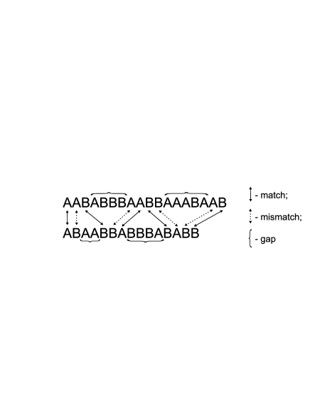
Figure 3: Matches, mismatches and gaps in a pair of sequences corresponding to the configuration of two random heteropolymers shown in Fig.1.

It is known Hwa97 ; HWA2 that the ground state energy

$$\tilde{\cal S}^{\rm max}=\max\left[N_{\rm match}+\gamma N_{\rm mis}\right]$$ (19)

satisfies the recursion relation

$$\tilde{\cal S}^{\rm max}_{m,n}=\max\left[\tilde{\cal S}^{\rm max}_{m-1,n},\,\tilde{\cal S}^{\rm max}_{m,n-1},\,\tilde{\cal S}^{\rm max}_{m-1,n-1}+\zeta_{m,n}\right]$$ (20)

with

$$\zeta_{m,n}=\begin{cases}1&\mbox{in case of match}\\ \gamma&\mbox{in case of mismatch}\end{cases}$$ (21)

Indeed, the ground state may correspond either (i) to the last two monomers connected, then the ground state energy equals $\tilde{\cal S}^{\rm max}_{m-1,n-1}+\zeta_{M,N}$, or (ii) to the unconnected end monomer of the fist (or second) chain, then the ground state energy is $\tilde{\cal S}^{\rm max}_{m,n-1}$ (or $\tilde{\cal S}^{\rm max}_{m-1,n}$).

Comparing Eqs(20), (21) with Eqs.(10), (11) one sees that they are identical up to the exchange of variables $\gamma\leftrightarrow a$. This establishes the analogy between initial heteropolymer problem formulated in (1)–(2) in the low–temperature limit (10) and the standard matching problem with general cost function (14).

For a pair of fixed sequences of lengths $m$ and $n$, the cost function $\tilde{\cal S}^{\rm max}_{m,n}$ is just a number. In the stochastic version of the LCS problem one compares two random sequences drawn from alphabet of $c$ letters and hence the cost function $\tilde{\cal S}^{\rm max}_{m,n}$ is a random variable. We are interested in the computation of the expectation and the variance of $\tilde{\cal S}^{\rm max}_{m,n}$ for $m=n\gg 1$ and the interpretation of the obtained results for LCS in terms of initial problem of unzipping of two random heteropolymers.

III.3 Bernoulli model for heteropolymers

We should note that the variables $\tilde{\eta}_{m,n}$ in (8) are not independent of each other. Actually, consider a simple example of two strings $\alpha={\rm AB}$ and $\beta={\rm AA}$. One has by definition: $\tilde{\eta}_{1,1}=\tilde{\eta}_{1,2}=1$ and $\tilde{\eta}_{2,1}=0$. The knowledge of these three variables is sufficient to predict that the last two letters do not match each other, i.e., $\tilde{\eta}_{2,2}=0$. Thus, $\tilde{\eta}_{2,2}$ can not take its value independently of $\tilde{\eta}_{1,1},\,\tilde{\eta}_{1,2},\,\tilde{\eta}_{2,1}$. These residual correlations between the $\tilde{\eta}_{i,j}$ variables make the LCS problem very complicated. However for two random sequences drawn from the alphabet of $c$ letters, the correlations between the $\tilde{\eta}_{m,n}$ variables vanish for $c\to\infty$.

In our work we restrict ourselves with the so-called Bernoulli matching (BM) model Monvel (which is simpler but yet nontrivial variant of the original LCS problem) where one ignores the correlations between $\tilde{\eta}_{m,n}$ for all $c$. The cost function $\tilde{F}_{m,n}^{BM}$ of the BM model satisfies the same recursion relation (8) except that the $\tilde{\eta}_{m,n}$’s are now independent variables, each drawn from the bimodal distribution:

$$\tilde{\eta}=\begin{cases}a&\mbox{with probability $P(\tilde{\eta})=1-\frac{1}{c}$}\vskip 6.0pt plus 2.0pt minus 2.0pt\\ 1&\mbox{with probability $P(\tilde{\eta})=\frac{1}{c}$}\end{cases}$$ (22)

As it has been already said, this approximation is expected to be exact only in the appropriately taken $c\to\infty$ limit. Nevertheless, for finite $c$, the results on the BM model can serve as a useful benchmark for original LCS model to decide if indeed the correlations between $\tilde{\eta}_{m,n}$ are important or not.

Note that the problem under discussion can be redefined as follows. Consider a matrix $\tilde{\eta}$ of size $m\times n$ and let the elements of this matrix be independent random variables with bimodal distribution (22). Consider now all directed paths in this matrix, i.e. ordered sequences $\{(m_{1},n_{1});(m_{2},n_{2});...;(m_{k},n_{k})\}$ such that $m_{i}>m_{i-1}$ and $n_{i}>n_{i-1}$ for $i=2,...,k$. Calculating the ground state energy of the matching problem is obviously equivalent to maximizing the sum of the matrix elements along these directed trajectories:

$$E_{m,n}(a)=\max_{\text{all sequences}}\sum_{i=0}^{k}\tilde{\eta}_{m_{i},n_{i}}$$ (23)

In Fig.4 we show an example of the evolution of the optimal path with the increase of $a$ for some particular random distribution of weights ”a” and ”1” (shown by white and grey squares respectively) corresponding to $c=4$.

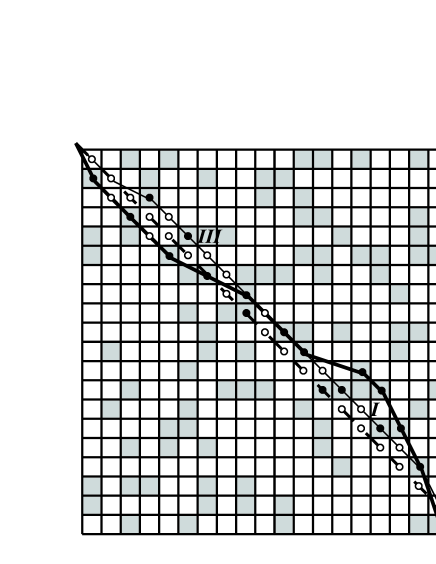
Figure 4: An example of a random distribution of ”1”s (gray squares) and ”$a$”s (white squares) on a $20\times 20$ matrix with $c=4$. The optimal path for $a=0$ is shown by the thick line, the diagonal optimal path for $a=1$ – by the dashed line and the evolution of the optimal path with increase of $a$ – by thin line. The ”1”s and ”$a$”s lying on the optimal paths are additionally marked by filled and open circles, respectively. See the main text for more details.

The optimal path for small $a$ is drawn in bold in Fig.4. With the increase of $a$, the first change in the optimal path configuration happens at $a=\frac{1}{3}$ when a shortcut I (shown by a thin line) is formed instead of the corresponding section of the bold line. Then, at $a=\frac{1}{2}$ the shortcut marked by II actuates, then at $a=\frac{2}{3}$ the one marked by III comes into play. So, for $a>\frac{2}{3}$ the optimal path is III–I–II. In what follows we call this kind of path subdiogonal, meaning that it goes only through the diagonal of the matrix ($a_{i,i}$ for $i=1,...,n$) and one of its subdiagonals ($a_{i,i+1}$, or $a_{i+1,i}$ for $i=1,...,n-1$). Finally, at $a=\frac{5}{6}$ the subdiagonal path III–I–II ceases to be the optimal one, and optimal path sticks to the diagonal (dashed line) where it stays up to $a=1$.

IV Expectations of LCS energy for general cost function $\tilde{\cal S}$

In this Section we consider the dependence of the ground state energy on the parameter $a$ defined in Eqs.(21)–(12). We start with the consideration of the limiting cases: (i) $a\ll 1$ and (ii) $\epsilon=1-a\ll 1$ and then, with the physical insight in hands, proceed to the semi–quantitative consideration of the general case.

IV.1 The case $0<a=\frac{u}{v}\ll 1$

In the limit $a=0$, as we have mentioned before, the problem under consideration corresponds exactly to the simplest version of the Longest Increasing Subsequence (LCS) problem, where the mismatches have no cost at all. The Bernoulli Matching model for this problem has been considered in details in nech_maj . An example of the random matrix with the optimal path is outlined by the bold line in Fig.4 (only filled circles, i.e. points with the weight equal to 1 are relevant in this case). We know that the ground state energy, $E_{m,n}$, as a function of the chain lengths $m,n$ behaves asymptotically for large $m$ and $n$ as

$$E_{m,n}(c,a=0)=\frac{2\sqrt{pmn}-p(m+n)}{q}+\frac{(pmn)^{1/6}}{q}\left[(1+p)-\sqrt{\frac{p}{mn}}(m+n)\right]^{2/3}\chi$$ (24)

where $p=c^{-1}$, $q=1-p$ and $\chi$ is a random variable with the Tracy–Widom distribution TW . The ground state energy, $E_{m,n}(a=0)$, has a meaning of the LIS length of ”1” (see nech_maj ). The mean value $\left<E_{m,n}\right>$ in the thermodynamic limit $n=m\to\infty$ equals to

$$\left<E_{m,n}\right>\equiv\left<E_{n,n}\right>=2\frac{\sqrt{p}-p}{q}n=\frac{2}{1+\sqrt{c}}n$$ (25)

Consider now the case of finite $a=\frac{u}{v}$ paying special attention to the effects of finite values of $m,n$ on typical fluctuations of $E$. We assume below $m=n$ for simplicity.

If the value of $a$ is small but finite ($0<a=\frac{u}{v}\ll 1$, the meaning of ”small” is specified below), then the trajectory of the optimal matching path does not change with respect to the case of $a=0$. The only difference from the $a=0$ case is that there are mismatches inserted between the matches whenever it is possible (see open circles along the bold line in Fig.4). It is not difficult to estimate the number of such inserted mismatches. Namely, the typical distance $\left<d\right>$ between the consequent ”1” (i.e. gray squares) along the optimal path in Fig.4 projected to the horizontal and vertical axes is, correspondingly, $\left<m_{i+1}-m_{i}\right>$ and $\left<n_{i+1}-n_{i}\right>$. The value of $\left<d\right>$ is dictated by the density of black circles along the optimal path (see fig.Fig.4). For $m=n\to\infty$ one has

$$\left<d\right>=\langle m_{i+1}-m_{i}\rangle=\langle n_{i+1}-n_{i}\rangle=\frac{n}{\left<E_{n,n}\right>}=\frac{1+\sqrt{c}}{2}$$ (26)

The average energy gain due to $a$’s (i.e. white squares in Fig.4) inserted into the optimal path can be estimated as follows

$$\left<\Delta E\right>=\left<E_{n,n}\right>\Big{(}\left<\min[m_{i+1}-m_{i},\;n_{i+1}-n_{i}]\right>-1\Big{)}a$$ (27)

Indeed, we can insert a white square into the optimal path between consequent gray squares if and only if the distance between these consequent gray squares in each of the dimensions is bigger or equal than two (we measure the distance in elementary squares). Let us estimate $\left<\Delta E\right>$ from above and from below.

1. The upper bound corresponds to the assumption that the increments of $m$ and $n$ are fully correlated. In this case $\left<\min[m_{i+1}-m_{i},\;n_{i+1}-n_{i}]\right>=\left<d\right>$ with $\left<d\right>$ computed in (26). Therefore, for $\left<\Delta E\right>$ we obtain the following estimate

$$\left<\Delta E\right><\left<E_{n,n}\right>\Big{(}\left<d\right>-1\Big{)}a=\left(1-\frac{2}{1+\sqrt{c}}\right)na$$ (28)

2. The construction of the lower bound corresponds to the assumption that the increments of $m$ and $n$ are completely independent. The computations in this case are slightly more involved since we have to compute explicitly the average value of the minimum $d_{\min}$ of two independent increments $m$ and $n$. The computations presented in the Appendix A lead us to the following lower bound of $\left<\Delta E\right>$:

$$\left<\Delta E\right>>\left<E_{n,n}\right>\Big{(}\left<d_{\min}\right>-1\Big{)}a=\left(\frac{1+\sqrt{c}}{2\sqrt{c}}-\frac{2}{1+\sqrt{c}}\right)na$$ (29)

Collecting (28) and (29) we arrive at the following bilateral estimate of $\left<\Delta E\right>$ for $0<a\ll 1$:

$$\left(\frac{1+\sqrt{c}}{2\sqrt{c}}-\frac{2}{1+\sqrt{c}}\right)a<\frac{\left<\Delta E\right>}{n}<\left(1-\frac{2}{1+\sqrt{c}}\right)a$$ (30)

It is worthwhile to notice in advance that, according to the numerical simulations, the genuine values of $\left<\Delta E\right>/n$ are actually very close to the lower bound (29).

IV.2 The case $a=1-\epsilon$ ($0<\epsilon\ll 1$)

Turn now to the opposite situation, $a=1-\epsilon$ ($0<\epsilon\ll 1$). For $\epsilon=0$ the situation is trivial. Indeed, there is no difference between ”1”s and ”$a$”s (i.e., gray and white squares at Fig.4 are identical) and the optimal path is thus the diagonal one with the energy

$$E(m,n)\equiv\min[m,n];\;\;E(n,n)\equiv n$$ (31)

Now, for small but finite $\epsilon$ and not too long trajectories, $n$ (the definition of ”not too long” is, once again, to be given below), the longest possible path still sticks to the main diagonal (see Fig.4). This path is optimal with the ground state energy given by

$$E^{\rm diag}_{n}(a)=n-k\epsilon$$ (32)

where $k$ is the number of $a$’s on the diagonal, which is a random variable distributed with the binomial law

$$W(k,n)=\frac{n!}{k!(n-k)!}q^{k}p^{n-k}$$ (33)

(recall that $q=1-\frac{1}{c}$ and $p=\frac{1}{c}$). Hence the average energy $\left<E^{\rm diag}_{n}\right>$ per monomer on the diagonal path equals

$$\frac{1}{n}\left<E^{\rm diag}_{n}\right>=1-\frac{\left<k\right>}{n}\,\epsilon=1-\left(1-p\right)\epsilon$$ (34)

Let us estimate now the length, $n_{\rm d}$, on which the optimal path detaches from the main diagonal. The optimal path of length $n$ is separated from each of the suboptimal ones (i.e., those of length $n-1$) by the energy gap $\delta E$:

$$\delta E=(n-k\epsilon)-(n-1-k^{\prime}\epsilon)=1-\epsilon\,\delta k$$ (35)

where $\delta k=k-k^{\prime}$ is the difference in the number of $a$’s on the optimal (diagonal) path and on the best of the suboptimal paths of lengths $n-1$ (see Fig.4). The optimal path detaches from the diagonal when $\delta E<0$. Since $\delta k$ cannot exceed $n-1$, the diagonal path is always optimal until

$$1-\epsilon\,\delta k<0\quad\Rightarrow\quad 1-(n_{\rm d}-1)\epsilon<0\quad\Rightarrow\quad n_{\rm d}>\epsilon^{-1}+1$$ (36)

where $n_{\rm d}$ is the length of the optimal path which detaches from the diagonal at energy $\epsilon$. The inequality (36) gives rather crude lower bound for the value of $n$ for which the detachment of the optimal path from the diagonal actually happens. To acquire better bounds we should take into account the concurrent effects involved. On one hand, the single diagonal path has the advantage of being the longest one. The corresponding value of $k$ has a binomial distribution (33) with the mean $\left<k\right>=nq$. On the other hand, the suboptimal paths (i.e., those of lengths $n-1$) are disadvantageous because they are shorter, however their intrinsic advantage consists in high degeneracy: one has many such suboptimal trajectories. The number $k^{\prime}$ of $a$’s on each particular suboptimal path is a binomial distributed random variable with the probability density $W(k^{\prime},n-1)$ and the mean $\left<k^{\prime}\right>=(n-1)q$. Now we have to find the best (i.e. the minimal) value $\left<k^{\prime}\right>$ among ${\cal N}$ suboptimal paths. These suboptimal paths (there are ${\cal N}\sim n^{2}/2$ of them) are, however, not independent. It is easy to understand that the number of independent suboptimal paths, $N_{\rm ind}$, satisfies the following bilateral inequality:

$$2\leq N_{\rm ind}\leq 3n-2$$ (37)

Indeed, on one hand, there are at least 2 independent paths coinciding with upper and lower subdiagonals. On the other hand, by definition, the suboptimal paths can visit only these two subdiagonals and the main diagonal itself. The corresponding energetic costs are therefore always linear combinations of the values on the diagonal ($n$) and two subdiagonals ($(n-1)$), that is, $n+2(n-1)=3n-2$ accessible matrix elements, which are themselves independent random variables. Evidently one cannot construct more than $3n-2$ independent linear combinations out of $3n-2$ independent variables. We are, hence, to compute the average minimum of $N_{\rm ind}$ independent random quantities each distributed with the probability density $W(k^{\prime},n-1)$. This task is solved in Appendix B. Taking into account the inequality (37) which defines the boundaries of $N_{\rm ind}$, we can get the upper and lower estimates for $\left<\delta k_{N_{\rm ind}}\right>$ ($n\gg 1$), where $\left<\delta k_{N_{\rm ind}}\right>$ is defined as follows:

$$\left<\delta k_{N_{\rm ind}}\right>=\left<k\right>-\left<k^{\prime}_{N_{\rm ind}}\right>\equiv npq-\left<k^{\prime}_{N_{\rm ind}}\right>$$ (38)

Substituting into (38) the expressions derived in Appendix B for $\left<k^{\prime}_{N_{\rm ind}}\right>$, we have:

$$q+\frac{1}{\sqrt{\pi}}(npq)^{1/2}<\left<\delta k_{N_{\rm ind}}\right><q+(2npq)^{1/2}\left[\ln\left(3n^{3/2}(pq)^{1/2}\right)\right]^{1/2}$$ (39)

Remembering now that the optimal path detaches from the diagonal at $\left<\delta k_{N_{\rm ind}}\right>\sim\epsilon^{-1}$, and dropping out all constants of order of one, we arrive for $n\gg 1$ at the following approximate bilateral estimate for the detachment length, $n_{\rm d}$:

$$n_{\rm d}\lesssim\left(\epsilon^{2}pq\right)^{-1}\lesssim n_{\rm d}\ln n_{\rm d}$$ (40)

In Fig.5 we show the results of our computer simulation of the average energy of the optimal path as a function of the sequence length for different values of $a$ and $p$. One notes the crossover (for fixed $a$ and $p$) from the path sticking to the diagonal at low $n$ and the high–$n$ regime, where the optimal path is detached. For $n\gg 1$ the average energy of the path eventually saturates at some value $E_{\infty}$, which is $a$– and $p$– dependent. Moreover, though the detachment point is not exactly well–defined, the rescaling according to the inequality (40) shows that it gives rather decent estimate of the detachment point. Note also that the plateau region persists up to quite large values of $\epsilon$. Indeed, it is easy to see from (36) that the detachment happens at $n_{d}>2$ (and thus a plateau of at least two points exists) for any $a>a_{d}=1/2$. It is less obvious and more important, however, that the more accurate estimate (40) is still relevant in the whole range of $a\in(1/2,1)$.

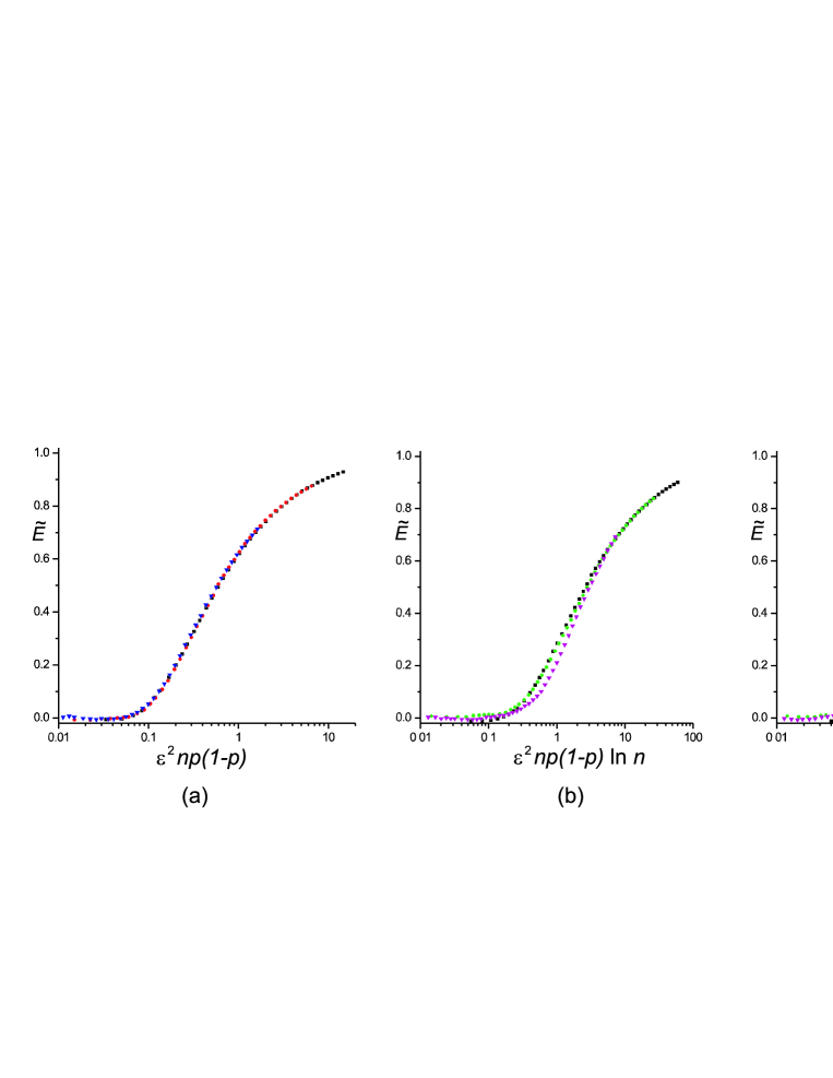
Figure 5: The dependence of the reduced mean energy $\tilde{E}=(\left<e_{n}\right>-\left<e_{0}\right>)/(\left<e_{\infty}\right>-\left<e_{0}\right>)$ of the optimal path on the reduced size $n$ of the system. (a) for $c=4$ and $\epsilon=0.3$ (black squares), $\epsilon=0.2$ (red circles), and $\epsilon=0.1$ (blue triangles); (b) and (c) for $\epsilon=0.2$ and $c=2$ (black squares), $c=8$ (green circles), and $c=32$ (magenta triangles). Note that curves for $c=2,8$ almost collapse after rescaling prescribed by the r.h.s of (40), while those for $c=8,32$ collapse with rescaling prescribed by the l.h.s. of (40).

IV.3 The general case $a\in[0,1]$: energy cost and fluctuations.

Consider now the general case of $a\in[0,1]$. In Fig.6 we present the estimates of the average ground state energy $\left<e_{n}(c,a)\right>=\left<E_{n}(c,a)\right>/n$ for different values of $c$ and $a$. These estimates we obtain by the finite size scaling extrapolating $\left<e_{n}(c,a)\right>$ from large, but finite, $n$ to $n\to\infty$.

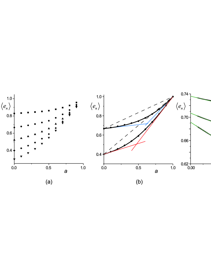
Figure 6: (a) The limiting value of the ground state energy per cite $\left<e_{n}(a)\right>\equiv\left<E(a)\right>/n$ as a function of $a$ for different $c$: $c=2$ (squares), $c=4$ (circles), $c=8$ (up triangles), $c=16$ (diamonds), $c=32$ (down triangles); (b) The upper (dashed line) and lower (thin solid lines) bounds and the hyperbolic fit (thick line) of the $\left<e_{n}(a)\equiv\left<E(a)\right>/n\right>$ dependence for $c=4$ (circles) and $c=16$ (diamonds); (c) The examples of the ground state energy per cite $\left<e_{n}\right>$ as a function of $n^{-2/3}$ (thick line) and the finite–size scaling fits used to obtain points in the figure a) (thin lines) for several different values of $a$ and $c$, line 1: $a=0.2,c=4$, line 2: $a=0.6,c=8$, line 3: $a=0.7,c=16$.

In our construction we use the following conjecture. One sees from (24) that at $a=0$ and for $m=n\gg 1$ the average ground state energy, $\left<e_{n}(c,a=0)\right>$, converges to its value at infinity, $\left<e_{\infty}(c,a=0)\right>=\frac{2}{1+\sqrt{c}}$, with the scaling exponent $\alpha=-2/3$:

$$\left<e_{n}(c,a=0)\right>=\frac{1}{n}\left<E_{n,n}(c,a=0)\right>=\frac{2}{1+\sqrt{c}}+\frac{c^{1/6}(\sqrt{c}-1)}{\sqrt{c}+1}\left<\chi\right>n^{-2/3}=\left<e_{\infty}(c,a=0)\right>+f(c)\left<\chi\right>n^{\alpha}$$ (41)

where $\left<\chi\right>=-1.7711...$ (see TW ).

We assume that the critical exponent $\alpha$ is $a$–independent and the finite size scaling of $\left<e_{n}(c,a)\right>$ for $a>0$ and $n\gg 1$ reads (see also Hwa97 )

$$\left<e_{n}(c,a)\right>=\left<e_{\infty}(c,a)\right>+g(c,a)\left<\chi\right>n^{\alpha}$$ (42)

where $g(c,a)$ is some function of $c$ and $a$, but not of $n$. Extrapolating the data of $\left<e_{n}(c,a)\right>$ computed numerically for large finite $n$ to $\left<e_{\infty}(c,a)\right>$ on the basis of finite size scaling (42), we arrive at the family of curves $\left<e_{\infty}(c,a)\right>$ for $c=2,4,8,16,32,64$ shown in Fig.6a,b. The results presented in Fig.6c, as well as those of Hwa97 demonstrate that the conjecture (42) is actually plausible. Apart from the points obtained by numerical simulation, in Fig.6b we depict: a) the estimates for $\left<e_{\infty}(c,a)\right>$ at small $a$ given by the inequality (30), and b) the estimates of $\left<e_{\infty}(c,a)\right>$ on the plateau for $a\to 1$ (Eq.(34)).

One should note that the numerical results for $a\ll 1$ are very close to the lower bound of (30). We use this fact to produce a fit for the dependence $\left<e_{\infty}(c,a)\right>$ in the whole range of parameter $a\in[0,1]$ for few values of $c$ ($c=4,16,64$). Namely, we fit the data of $\left<e_{\infty}(a)\right>$ by a hyperbola of general form

$$(\left<e_{\infty}(a)\right>+\kappa_{1}a+\delta_{1})(\left<e_{\infty}(a)\right>+\kappa_{2}a+\delta_{2})=R$$ (43)

with the constraints that this hyperbola passes through the points $(a,e_{\infty}(a))=(0,2/(\sqrt{c}+1))$ at $a=0$, and $(a,e_{\infty}(a))=(1,1)$ at $a=1$ with the slopes given by limiting linear approximations (30) and (34) correspondingly. These four constraints leave us effectively with only one free parameter, which we change to arrive at the best fit of the experimental data. As one sees from Fig.6b, the found fits for different values of $c$ are quite good.

Let us now discuss briefly the fluctuations of the average free energy and their dependence on $n$. One expects for $n\gg 1$ the average fluctuations $\sigma^{2}_{E}$ to be proportional to $n^{2/3}$, typical for the Kardar–Parisi–Zhang universality class Hwa97 . This conjecture is consistent with the computation of the fluctuations of the averaged length of the Longest Common Subsequence (LCS) in the $a=0$ limit for Bernoulli Matching model (see nech_maj ):

$$\sigma^{2}_{E}(n)={\rm Var}\,E_{n,n}(c)=\left<E_{n,n}^{2}(c)\right>-\left<E_{n,n}(c)\right>^{2}\approx\left(\langle\chi^{2}\rangle-{\langle\chi\rangle}^{2}\right)\,f^{2}(c)\,n^{\theta_{0}}$$ (44)

where $\theta_{0}=2/3$ and $\langle\chi^{2}\rangle-\langle\chi\rangle^{2}=0.8132\dots$.

The behavior for intermediate values of $n$ is more involved. In particular, for small $a$ and intermediate $n$ one expects for $\sigma^{2}_{E}(n)$ the growth with the critical exponent $\theta_{1}$:

$$\sigma^{2}_{E}(n)\sim n^{\theta_{1}}$$ (45)

The exponent $\theta_{1}$ is known to be typical for the ”transitional” regime in the (1+1)D KPZ equation Krug ; Krech . In terms of the work Krech the exponent $\theta_{1}$, which governs the short–time behavior of the correlation function of KPZ model, is $\theta_{1}=(d+4)/z-2$, where $z$ is the dynamic exponent Krech , and $d$ is the space dimensionality. In $d=1$ the value of $z$ for KPZ model is known exactly, $z=3/2$, giving the value $\theta_{1}=4/3$.

For $a=1-\epsilon$ ($\epsilon\ll 1$) the plateau regime for $e_{n}(c,a)$ exists at low $n\lesssim n_{\rm d}$ (where $n_{\rm d}$ is defined in (40)). The arguments of Section IV.2 allow us to expect the in this case the variance $\sigma^{2}_{E}(n)$ behaves as

$$\sigma^{2}_{E}(n)\sim n^{\theta_{2}}$$ (46)

with the Gaussian exponent $\theta_{2}=1$ since the plateau energy is just the sum of $n$ independent random variables.

The numerical results presented in Fig.7 for $\sigma^{2}_{E}(n)$ fully confirm the behaviors (44), (45) and (46). In the case of intermediate $a$ shown in Fig.7c the sequence of regimes, at least for large $c$ is more reach: we first note the exponent $\theta_{2}=1$ (plateau), then the exponent $\theta_{1}=4/3$ (”transitional” KPZ), and finally the exponent $\theta_{0}=2/3$ (large scale KPZ). It looks like the growing plateau region continuously ”swallows up” the finite–size KPZ region with the increase of $a$, and thus at $\epsilon=1-a\ll 1$ one sees only two regimes.

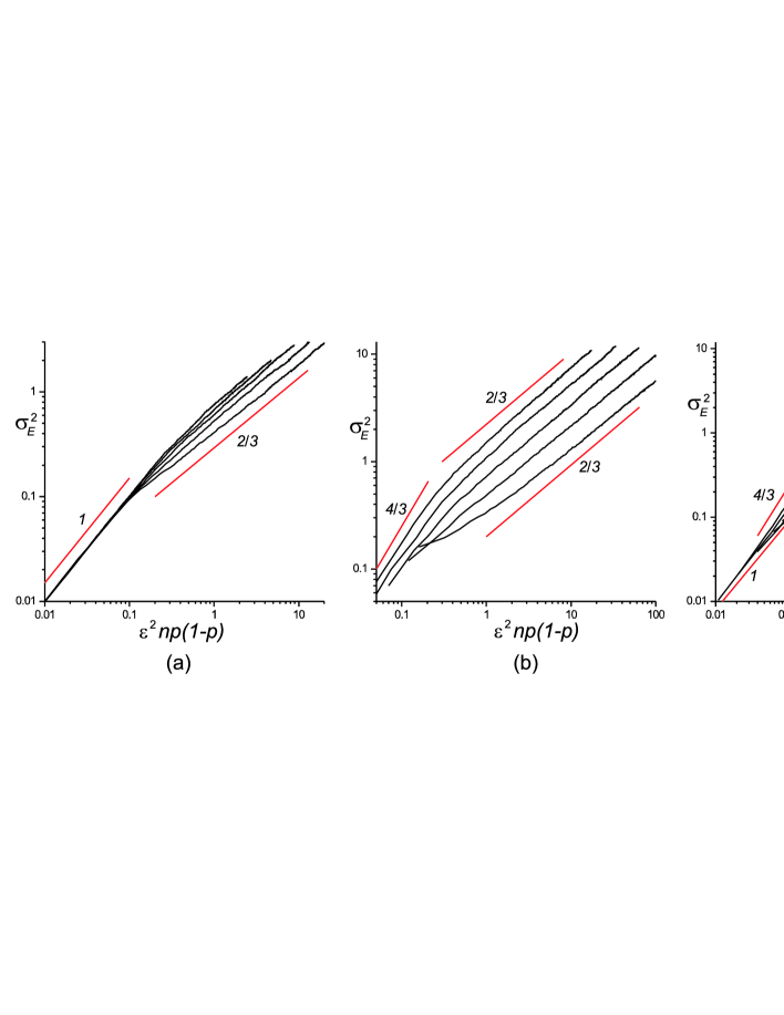
Figure 7: The dispersion $\sigma_{E}$ of the ground state energy as a function of $N$ for different values of $a$ and $c$. (a) $a=0.7$, (b) $a=0.2$, (c) $a=0.4$. In all figures $c=2,4,8,16,32$ in ascending order.

The important question concerning the results presented above is how universal are they with respect to the change of the model settings. Indeed, the exponents $\theta_{0,1,2}$ are obtained in the assumption of Bernoulli matching, i.e. assuming the contact matrix $\beta$ doesn’t have any correlations in it. As it was mentioned above, in reality it is not the case. Though we assume that some of the exponents may be universal, and may even hold in the case when there are strong long-range correlations in the structure of the associating DNA strands, the situation is a priori very unclear, a thorough numerical investigation of this question would be, in our opinion, an essential contribution in the field of the KPZ-related studies.

V Conclusion

In this work we have analyzed the average normalized ground state energy, $e$, of the complex of two random heteropolymers with quenched sequences as a function of chain length, $n$, in the ensemble of chains with uniform distribution of primary structures. The main attention is paid to the behavior of the function $e(n)$ at intermediate chain lengths and low temperatures.

The dependence $\left<e_{n}\right>$ is shown in Fig.5. Besides the formal estimates of the boundaries (30), (34), and of the crossover length, $n_{\rm d}$ (Eq.(40)), it seems to be desirable to acquire the qualitative understanding of the zipping energy $\left<e_{n}\right>$ for different chain lengths and different values of $a$.

One sees that the normalized energy $\left<e_{n}\right>$ for relatively long ($n>n_{\rm d}$) zipped chain configurations, is larger than the corresponding energy in a hairpin state for $n<n_{\rm d}$. The reason for this result is as follows. Longer chains could optimize their energy matching via loops creation while for short chains the penalty for loop formation is forbiddingly large. Hence the inequality (40) gives the criterium for characteristic scale length which separates two kinds of structure behavior: short chains form the hairpin configuration in which the monomers are forced to bond without any regard of their species, while long chains are capable of adjusting their spatial configurations by loop formation to obtain better matching. The crossover around $n_{\rm d}$ is, thus, separating the small $n$ region where the energy approaches the plateau value (34) exponentially fast with decreasing $n$, and infinitely large region of increasing $\left<e_{n}\right>$ where it approaches its value at $n\to\infty$ with the power low dependence $\left<e_{\infty}\right>-\left<e_{n}\right>\sim n^{-2/3}$. This behavior of $\left<e_{n}\right>$ depends only qualitatively (see (40)) on the parameter $a$ for sufficiently large $a>a_{\rm d}\sim 0.5$.

The unzipping process of two random heteropolymer chains is schematically shown in Fig.8. The results of previous sections allow us to find the dependence of the force $f(x)$ per chain monomer, on an average extension distance, $x$, between chain ends. If $N$ is the total length of each heteropolymer chain, and $n$ is the average current length of the heteropolymer complex measured from its common bottom end (see Fig.8), then by construction, $x=2(N-n)$. For the sake of simplicity, we neglect here the fluctuations of the unzipped regions of the chain.

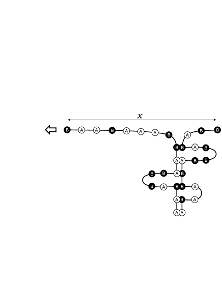
Figure 8: Unzipping of two random heteropolymers.

The plot of the average force, $f$, per chain monomer on the average separation distance, $x$, is shown in Fig.9. To be precise, $f(x)$, is the force necessary to unzip two random heteropolymer chains whose ends are separated by the distance $x$ averaged over all equally distributed primary structures at low temperatures for fixed value $a=\frac{v}{u}$ and given number of letters in the alphabet, $c$. The function $f(x)$ can be easily obtained from the dependence $\left<e_{n}\right>$ shown in Fig.6. Namely, $f(x)=\frac{d}{dn}(n\left<e_{n}\right>)$ at $n=N-x/2$.

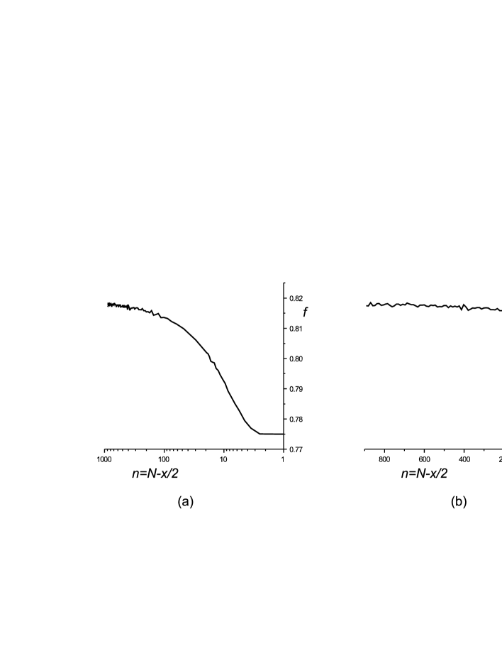
Figure 9: Dependence of unzipping force, $f$, per chain monomer on average separation distance, $x$. (a) log-linear scale, (b) linear scale.

Qualitative explanation of this phenomenon repeats the above discussion of the ground state free energy $\left<e_{n}\right>$. As it has been said already, the main attention in our work is paid to relatively small $n$, i.e. large average separation distances, $x$. (For discussions of the peculiarities of the force on the other bound, i.e. at $x\to 0$, see singh .) When $x$ approaches the contour length, $2N$, the equilibrium unzipping force $f(x)$ gradually decreases as $const-n^{-2/3}=const-(N-x/2)^{-2/3}$ until $N-x/2\sim n_{d}$ when the force drops further down to reach the limiting plateau value (34) where it saturates independently of further increase of $x$.

Let us stress once more that the result obtained is valid only for values of $f(x)$ averaged over the ensemble of realizations of different heteropolymer sequences: for any given heteropolymer sequence, the equilibrium force would be a highly fluctuating function of the distance $x$. In reality, moreover, the unzipping experiments are often set up in the fixed-force ensemble, instead of the fixed-distance one (see, for example, Cocco1 ; Cocco2 ), i.e. the constant force is applied to the ends of the chain, and the dynamics of the unzipping under this constant force is studied. In such a setting the knowledge of the characteristic occupation times for the intermediate states allows to reconstruct the overall free energy landscape. We predict that after the averaging over many realizations of such an experiment with different primary structures, one expects the typical occupation times for almost unzipped intermediate states to be less than those for the almost zipped conformations (the particular difference depends on the applied force). Correspondingly, the life time of the intermediate states is gradually decreasing with the increase of $x$ until saturating at $N-x/2\sim n_{d}$.

Appendix A Average value of the minimum of two independent increments

First of all we should make a conjecture about the distribution of intervals $d_{m}=m_{i+1}-m_{i}$ and $d_{n}=n_{i+1}-n_{i}$. It seems to be rather natural to suppose that the intervals $d_{m,n}$ have the exponential distribution, i.e. $p(d_{m,n})\sim e^{-kd_{m,n}}$ (one can easily check that at least the tails of this distribution are indeed exponential). Normalizing $p(d_{m,n})$, we get

$$p(d_{m,n})=\frac{e^{-kd_{m,n}}}{\sum\limits_{d_{m,n}=1}^{\infty}e^{-kd_{m,n}}}=(e^{k}-1)e^{-kd_{m,n}}$$ (47)

The mean values $\left<d_{m}\right>$ and $\left<d_{n}\right>$ are

$$\left<d_{m}\right>=\left<d_{n}\right>=\sum\limits_{d_{m,n}=1}^{\infty}d_{m,n}\;p(d_{m,n})=\frac{e^{k}}{e^{k}-1}$$ (48)

Now we are to find the averaged joined minimum $\left<d_{\min}\right>$ of two random variables $d_{m}$ and $d_{n}$ distributed with (47). To do that we proceed as follows. First of all find the discrete integral distribution function, $F_{1}(z)$, for each random distribution, $p(d_{m})$ and $p(d_{n})$:

$$F_{1}(z)=\sum\limits_{d_{m,n}=1}^{z}p(d_{m,n})=1-e^{-kz}$$ (49)

Following the general procedure, define now the joined discrete integral distribution function, $F_{2}(z)$,

$$F_{2}(z)=1-(1-F_{1}(z))^{2}=1-e^{-2kz}$$ (50)

Taking the discrete derivative, $p_{2}(z)=F_{2}(z)-F_{2}(z-1)$, we find the probability distribution, $p_{2}(z=d)$ for the minimum $d_{\min}=\min[m_{i+1}-m_{i},\;n_{i+1}-n_{i}]$. The last step consists in taking average $\left<d_{\min}\right>$ with respect to the joined distribution function $p_{2}(d)$:

$$\left<d_{\min}\right>=\sum_{z=1}^{\infty}z\,p_{2}(z)=\frac{e^{2k}}{e^{2k}-1}$$ (51)

Collecting (26), (48) and (51), we get

$$\left\{\begin{array}[]{l}\displaystyle\frac{e^{k}}{e^{k}-1}=\frac{1+\sqrt{c}}{2}\vskip 6.0pt plus 2.0pt minus 2.0pt\\ \displaystyle\frac{e^{2k}}{e^{2k}-1}=\left<d_{\min}\right>\end{array}\right.$$ (52)

and thus, resolving (52),

$$\left<d_{\min}\right>=\frac{(1+\sqrt{c})^{2}}{4\sqrt{c}}$$ (53)

Substituting (53) into (27) one obtains finally the estimate of $\Delta E$ from below:

$$\Delta E>\left<L_{n,n}\right>\Big{(}\left<d_{\min}\right>-1\Big{)}a=\left(\frac{1+\sqrt{c}}{2\sqrt{c}}-\frac{2}{1+\sqrt{c}}\right)na$$ (54)

Appendix B Auxiliary construction for estimation of the detachment length

Assuming $\frac{n}{c}\gg 1$ one can replace the binomial distribution (33) with the Gaussian one and approximate $W(k)$ as follows

$$\tilde{W}(k,n)=\frac{1}{\sqrt{2\pi npq}}\exp\left(-\frac{(k-\left<k\right>)^{2}}{2npq}\right)$$ (55)

where $\left<k\right>=nq$. The distribution function for the variable $k^{\prime}$ $W(k^{\prime},n-1)$ is completely similar but the replacement $n\to n-1$.

We are now to compute the mean minimal value $\left<k^{\prime}_{N_{\rm ind}}\right>$ of $N_{\rm ind}$ random variables, each distributed with $W(k^{\prime},n-1)\equiv W(k^{\prime})$. Repeating the same procedure as in the Appendix A, we proceed as follows. First of all pass to the integral distribution function, $\tilde{F}(z)$:

$$\tilde{F}(z)=\int_{-\infty}^{z}\tilde{W}(k^{\prime})dk^{\prime}=\frac{1}{2}\left(1+{\rm erf}\left[\frac{z-(n-1)q}{\sqrt{2(n-1)pq}}\right]\right)$$ (56)

Now construct the new probability distribution function, $Q(z)$, for the joint distribution, as follows:

$$Q(z)=\frac{d}{dz}\left[1-(1-\tilde{F}(z))^{N_{\rm ind}}\right]=N_{\rm ind}\,\tilde{F}^{\prime}(z)\,(1-\tilde{F}(z))^{N_{\rm ind}-1}$$ (57)

The desired mean minimal value $\left<k^{\prime}_{N_{\rm ind}}\right>$ reads now

$$\left<k^{\prime}_{N_{\rm ind}}\right>=\int_{-\infty}^{\infty}zQ(z)dz$$ (58)

Now, taking the estimate (37) into account one readily arrives to the lower bound for $\left<k^{\prime}_{N_{\rm ind}}\right>$. Indeed, for $N_{\rm ind}=2$

$$\left<k_{N_{\rm ind}}^{{}^{\prime}\min}\right>=\frac{1}{\sqrt{\pi}}\int_{-\infty}^{\infty}\left(y\sqrt{2(n-1)pq}+(n-1)q\right)e^{-y^{2}}\Big{(}1-{\rm erf}(y)\Big{)}dy=(n-1)q-\frac{1}{\sqrt{\pi}}\Big{(}(n-1)pq\Big{)}^{1/2}$$ (59)

For $N_{\rm ind}=3n-2\gg 1$ (see (37)) the integral (58) cannot be computed analytically and therefore one needs to apply some approximative approach. We proceed as follows. The function $\tilde{F}(z)$ has a sense of the area under the curve $\tilde{W}(k)$ in the interval $k^{\prime}\in(-\infty,z]$. Consider now $N_{\rm ind}\gg 1$ independent random variables each distributed with $\tilde{W}(k^{\prime})$. For $\frac{z-(n-1)q}{\sqrt{(n-1)pq}}\ll-1$ on average one point of $N_{\rm ind}$ equally distributed random points lies in the area $\tilde{F}(z)\sim N_{\rm ind}^{-1}$. Since this area is the area under the left tail of the distribution $\tilde{W}(k^{\prime})$, the point inside this area is the minimal one by construction. So, expanding $\tilde{F}(z)$ for $\frac{z-(n-1)q}{\sqrt{(n-1)pq}}\ll-1$, we get

$$\tilde{F}(z)=\frac{1}{2}\left(1+{\rm erf}\left[\frac{z-(n-1)q}{\sqrt{2(n-1)pq}}\right]\right)\simeq\frac{\sqrt{(n-1)pq}}{\sqrt{2\pi}((n-1)q-z)}\exp\left(-\frac{(z-(n-1)q)^{2}}{2(n-1)pq}\right)\sim\frac{1}{N_{\rm ind}}$$ (60)

Since the term in the exponent in (60) varies much faster than the pre-exponential term, we can roughly estimate $z=\left<k_{N_{\rm ind}}^{{}^{\prime}\max}\right>$ as follows

$$\left<k_{N_{\rm ind}}^{{}^{\prime}\max}\right>\simeq(n-1)q-\Big{(}2(n-1)pq\Big{)}^{1/2}\left[\ln\left(N_{\rm ind}\Big{(}(n-1)pq\Big{)}^{1/2}\right)\right]^{1/2}$$ (61)

Note that Eq.(61) is obtained from Eq.(60) under the condition $z<(n-1)q$ which fixes the right sign of the square root branch of the second term in Eq.(61).

Substituting $N_{\rm ind}=3n-2$ into (61) and taking into account that $n\gg 1$, we get the following desired estimate for $\left<k_{N_{\rm ind}}^{{}^{\prime}\max}\right>$:

$$\left<k_{N_{\rm ind}}^{{}^{\prime}\max}\right>\simeq(n-1)q-(2npq)^{1/2}\left[\ln\left(n^{3/2}(pq)^{1/2}\right)\right]^{1/2}$$ (62)

Now we can use the boundaries (59) and (62) for getting lower and upper bounds of $\left<\delta k_{N_{\rm ind}}\right>$ and of the detachment length, $n_{\rm d}$ – see Eqs.(39)–(40).

References

- (1) S.M. Bhattacharjee, J. Phys. A: Math. Gen. 48, L423 (2000)
- (2) K.L. Sebastian, Phys. Rev. E 62, 1128 (2000)
- (3) D.K. Lubensky, D.R. Nelson, Phys. Rev. Lett. 85, 1572 (2000)
- (4) S. Cocco, R. Monasson, J.F. Marko, Proc. Nat. Acad. Sci. USA 98, 8608 (2001); Phys. Rev. E 65, 0141907 (2002)
- (5) D. Morenduzzo, S. Bhattacharjee, S. Maritan, E. Orlandini, F. Seno, Phys. Rev. Lett. 88, 028102 (2002)
- (6) D.K. Lubensky and D.R. Nelson, Phys. Rev. E 65, 031917 (2002)
- (7) D. Cule and T. Hwa, Phys. Rev. Lett. 79, 2375 (1997)
- (8) L.-H. Tang and H. Chate, Phys. Rev. Lett. 86, 830 (2001)
- (9) N. Singh, Y. Singh, Eur. Phys. J. 17, 7 (2005)
- (10) P. de Gennes, Biopolymers, 6, 715 (1968)
- (11) I.Ya. Erukhimovich, Vysokomolek. Soed., 20B, 10 (1978) – in Russian
- (12) M. Mueller, Phys. Rev. E, 67, 021914 (2003)
- (13) V. Guttal, R. Bundschuh, Phys. Rev. Lett 96, 018105 (2006)
- (14) R.A. Neher, U. Gerland, Phys. Rev. E, 73, 030902 (2006)
- (15) M. Tamm, S. Nechaev, Phys. Rev. E, 75, 031904 (2007)
- (16) L. Comtet, Advanced Combinatorics: The Art of Finite and Infinite Expansions, (Dordrecht: Reidel, 1974), pp. 80–81
- (17) D. Gusfield, Algorithms on Strings, Trees, and Sequences (Cambridge University Press, Cambridge, 1997)
- (18) J. Boutet de Monvel, European Phys. J. B 7, 293 (1999); Phys. Rev. E 62, 204 (2000)
- (19) S.B. Needleman and C.D. Wunsch, J. Mol. Biol. 48, 443 (1970)
- (20) T.F. Smith and M.S. Waterman, J. Mol. Biol. 147, 195 (1981); Adv. Appl. math. 2, 482 (1981)
- (21) M.S. Waterman, L. Gordon, and R. Arratia, Proc. Natl. Acad. Sci. USA, 84, 1239 (1987)
- (22) S.F. Altschul et. al., J. Mol. Biol. 215, 403 (1990)
- (23) D. Sankoff and J. Kruskal, Time Warps, String Edits, and Macromolecules: The theory and practice of sequence comparison (Addison Wesley, Reading, Massachussets, 1983)
- (24) A. Apostolico and C. Guerra, Alogorithmica, 2, 315 (1987)
- (25) R. Wagner and M. Fisher, J. Assoc. Comput. Mach. 21, 168 (1974)
- (26) V. Chvátal and D. Sankoff, J. Appl. Probab. 12, 306 (1975)
- (27) J. Deken, Discrete Math. 26, 17 (1979)
- (28) J.M. Steele, SIAM J. Appl. Math. 42, 731 (1982)
- (29) V. Dancik and M. Paterson, in STACS94, Lecture Notes in Computer Science, 775, 306 (Springer: New York, 1994)
- (30) K.S. Alexander, Ann. Appl. Probab. 4, 1074 (1994)
- (31) M. Kiwi, M. Loebl, and J. Matousek, in Lecture Notes in Computer Science, 2976 302 (Springer: Berlin, 2004)
- (32) M. Zhang and T. Marr, J. Theor. Biol. 174, 119 (1995).
- (33) T. Hwa and M. Lassig, Phys. Rev. Lett. 76, 2591 (1996)
- (34) R. Bundschuh, T. Hwa, Discrete Appl. Math. 104, 113 (2000).
- (35) S.N. Majumdar, S. Nechaev, Phys. Rev. E 72, 020901(R) (2005)
- (36) C.A. Tracy and H. Widom, Comm. Math. Phys. 159, 151 (1994); see also Proc. of ICM, Beijing, Vol. I, 587 (2002)
- (37) D. Drasdo, T. Hwa, M. Lassig, J. Comp. Biol. 7, 115 (2000)
- (38) J. Krug, Phys. Rev. A 44, R801 (1991)
- (39) M. Krech, Phys. Rev. E 55, 668 (1997)
- (40) V. Baldazzi, S. Cocco, E. Marinari, R. Monasson, Phys. Rev. Lett. 96, 128102 (2006)
- (41) V. Baldazzi, S. Bradde, S. Cocco, E. Marinari, R. Monasson, Phys. Rev. E 75, 011904 (2007)