Lensing and Supernovae: Quantifying The Bias on the Dark Energy Equation of State
Abstract
The gravitational magnification and demagnification of Type Ia supernovae (SNe) modify their positions on the Hubble diagram, shifting the distance estimates from the underlying luminosity-distance relation. This can introduce a systematic uncertainty in the dark energy equation of state (EOS) estimated from SNe, although this systematic is expected to average away for sufficiently large data sets. Using mock SN samples over the redshift range we quantify the lensing bias. We find that the bias on the dark energy EOS is less than half a percent for large datasets ( 2,000 SNe). However, if highly magnified events (SNe deviating by more than 2.5) are systematically removed from the analysis, the bias increases to 0.8%. Given that the EOS parameters measured from such a sample have a 1 uncertainty of 10%, the systematic bias related to lensing in SN data out to can be safely ignored in future cosmological measurements.
Subject headings:
cosmology: observations — cosmology: theory — supernova — parameter estimation — gravitational lensing1. Introduction
Since the discovery of the accelerating expansion of the universe (Riess et al., 1998; Perlmutter et al., 1999; Knop et al., 2003; Riess et al., 2004), the quest to understand the physics responsible for this acceleration has been one of the major challenges of cosmology. At present the dominant explanation entails an additional energy density to the universe called dark energy. The physics of dark energy is generally described in terms of its equation of state (EOS), the ratio of its pressure to density. In some models this quantity can vary with redshift. While there exist a variety of probes to explore the nature of dark energy, one of the most compelling entails the use of type Ia supernovae to map the Hubble diagram, and thereby directly determine the expansion history of the universe. With increasing sample sizes, SN distances can potentially provide multiple independent estimates of the EOS when binned in redshift (Huterer & Cooray, 2005; Sullivan, Cooray, & Holz, 2007; Sullivan et al., 2007). Several present and future SN surveys, such as SNLS (Astier et al., 2006) and the Joint Dark Energy Mission (JDEM), are aimed at constraining the value of the dark energy EOS to better than 10%.
Although SNe have been shown to be good standardizable candles, the distance estimate to a given SN is degraded due to gravitational lensing of its flux (Frieman, 1997; Wambsganss et al., 1997; Holz & Wald, 1998). The lensing becomes more prominent as we observe SNe out to higher redshift, with the extra dispersion induced by lensing becoming comparable to the intrinsic dispersion (of magnitudes) at (Holz & Linder, 2005). In addition to this dispersion, which leads to an increase in the error associated with distance estimate to each individual supernova, lensing also correlates distance estimates of nearby SNe on the sky, since the lines-of-sight pass through correlated foreground large-scale structure (Cooray, Huterer, & Holz, 2006; Hui & Greene, 2006). Although this correlation error cannot be statistically eliminated by increasing the number of SNe in the Hubble diagram, the errors can be controlled by conducting sufficiently wide-area () searches for SNe (in lieu of small-area pencil-beam surveys).
In addition to the statistical covariance of SN distance estimates, gravitational lensing also introduces systematic uncertainties in the Hubble diagram by introducing a non-Gaussian dispersion in the observed luminosities of distant SNe. Since lensing conserves the total number of photons, this systematic bias averages away if sufficiently large numbers of SNe per redshift bin are observed. In this case the average flux of the many magnified and demagnified SNe converges on the unlensed value (Holz & Linder, 2005). Nonetheless, even with thousands of SNe in the total sample it is possible that the averaging remains insufficient, given that one may need to bin the Hubble diagram at very small redshift intervals to improve sensitivity to the EOS. Furthermore, SNe at higher redshifts are more likely to be significantly lensed. If “obvious” outliers to the Hubble diagram are removed from the sample, this introduces an important bias in cosmological parameter determination, and can lead to systematic errors in the determination of the dark energy EOS.
In this paper we quantify the bias introduced in the estimation of the dark energy EOS due to weak lensing of supernova flux. We consider the effects due to the non-Gaussian nature of the lensing magnification distributions (Wang, Holz, & Munshi, 2002), performing Monte-Carlo simulations by creating mock datasets for future JDEM-like surveys. The paper is organized as follows: In 2.1 we discuss our parameterization of the dark energy EOS, 2.2 discusses gravitational lensing, and 3 is an in-depth description of our methodology. We present our results in 4.
2. Background
2.1. Parameter Estimation Using SNe Ia
For a SN with intrinsic luminosity , the distance modulus is given by
| (1) |
where, in the framework of FRW cosmologies, the luminosity distance is a function of the cosmological parameters and the redshift. We consider the two-parameter, time-varying dark energy EOS (Chevalier & Polarski, 2001; Linder, 2003) adopted by the Dark Energy Task Force (DETF) (Albrecht et al., 2006). We take a flat universe described by the cosmological parameters , with the dimensionless Hubble constant, the dimensionless matter density, and and the parameters describing the dark energy EOS . One can then express as
| (2) |
where is the Hubble parameter at redshift :
| (3) |
2.2. Weak Lensing of Supernova Flux
Light from a distant SN passes through the intervening large-scale structure of the universe. This causes a modification of the observed flux due to gravitational lensing:
| (4) |
where is the lensing induced magnification at redshift in the direction of the SN on the sky, , and is the flux that would have been observed in the absence of lensing. The magnification can be either greater than (magnified) or less than (demagnified) one, with corresponding to the (unlensed) pure FRW scenario.
This magnification (or demagnification) of the observed flux leads to an error in the distance modulus, which can be expressed as
| (5) |
where we have written as for brevity.
Even in the absence of lensing the measured distance modulus to a Type Ia SN suffers an intrinsic error, since the supernovae are not perfect standard candles. This error is typically taken to be a Gaussian distribution in either flux or magnitude, with a redshift-independent standard deviation of . On the other hand, as lensing intrinsically depends on the optical depth, which increases with redshift, the scatter (or variance) due to lensing also increases with redshift (Holz & Linder, 2005). The probability distribution function (PDF) for lensing magnification, , of a background source at redshift , depends on both the underlying cosmology and on the nature of the foreground structure responsible for lensing. We make use of an analytic form for that was calibrated with numerical simulations (Wang, Holz, & Munshi, 2002), which is valid for events that are not strongly lensed ( is less than a few).

The generic gravitational lensing PDF peaks at a demagnified value, with a long tail to high magnification (Wang, Holz, & Munshi, 2002; Sereno, Piedipalumbo, & Sazhin, 2002). However, since the total number of photons is conserved by lensing, all lensing distributions preserve the mean: . To ensure that this criterion is met (to an accuracy of one part in a million), we re-normalize the magnification PDF in a slightly different way than what was originally suggested in Wang, Holz, & Munshi (2002). is related, at a given redshift, to the probability distribution for the reduced convergence, , through (see Wang, Holz, & Munshi (2002); Eq. (6)), where is the minimum convergence. The free parameter in normalizing , and hence, , is , the maximum value for the reduced convergence. We determine the unique value of which yields both and (to better than ). Since the mode is not equal to the mean, the distribution is manifestly non-Gaussian. The majority of distant supernovae are slightly demagnified, and the inferred luminosity distances are skewed to higher values. The SN redshifts, on the other hand, remain unaffected, since gravitational lensing is achromatic. Although lensing magnification is insignificant at low redshifts, at redshifts above one both weak and strong lensing become more prominent. For small SN samples the overall bias is towards a larger cosmological acceleration (e.g., too large a value of for CDM models). The lensing also adds a systematic bias to estimates of the dark energy EOS, shifting to a more negative value of the EOS (e.g., less than for a universe with a cosmological constant). Along with a large fraction of demagnified SNe, lensing produces a small number of highly magnified sources. If this high-magnification tail can be well sampled, the average of the lensing distribution is expected to converge on the true mean, and the bias can be eliminated (Wang, 2000; Holz & Linder, 2005).
3. Methodology


We generate mock SN samples, and quantify the bias in the estimation of the dark energy EOS due to gravitational lensing. We pick as our fiducial cosmology a flat universe with , , , and with a Gaussian prior of . We consider a range of possible upcoming surveys, and Monte-Carlo SN samples of varying sizes distributed uniformly in the redshift range . If the SN intrinsic errors are Gaussian in flux, then it makes sense to analyze the data via flux averaging. In this case both the intrinsic errors and the lensing errors will average away for sufficiently large SN samples. However, if the intrinsic errors are Gaussian in magnitude, then a magnitude analysis may be more appropriate, although this will lead to a bias due to lensing (which is only bias-free for flux analysis). In what follows we perform both analyses.
3.1. Magnitude Analysis
For each SN at a redshift we draw a value of at random from the re-normalized lensing PDF, , obtained from Wang, Holz, & Munshi (2002), and use Eq. (5) to evaluate . To model the intrinsic scatter we draw a number at random from a Gaussian distribution of zero mean and standard deviation given by mag (Astier et al. (2006) find a scatter at the level of 0.13 mag). We combine the intrinsic and lensing noise with the “true” underlying distance modulus to get the observed distance modulus:
| (6) |
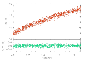
By repeating the above procedure for each of the SNe in a sample, we generate a mock Hubble diagram. We create mock surveys with different numbers of SNe: , 2000, & 10,000; and then for each fixed number of SNe we generate at least 10,000 independent mock samples to properly sample the distributions. In Figure 1 we show an example of one such dataset with a SNe sample size of 2000. The upper panel shows the Hubble diagram and the lower panel shows the residuals of the distance moduli relative to that of the fiducial cosmological model.
For each mock Hubble diagram we compute the likelihood of a parameter set by evaluating the -statistic:
| (7) |
where is the error bar for the distance modulus of the th supernova, taken to be 0.1 mag throughout. The projected bias in the estimation of can now be computed by marginalizing over and (keeping fixed).
3.2. Flux-Averaging Analysis
Wang (2000) argues that averaging the flux, as opposed to the magnitudes, of observed SNe naturally removes the lensing bias, since the mean of the lensing distributions are equal to one in flux, but not in magnitude. We thus also analyze the mock data sets in flux. The flux averaging is done such that for each supernova we first use Eq. (2) to calculate the value of , and then evaluate the fiducial flux using
| (8) |
where we can take any a priori fixed value of . We take the lensing PDF, , and convolve it with a Gaussian distribution having zero mean and dispersion 0.1 (this corresponds to 5% error in distance estimates). We then randomly draw from the convolved distribution, and multiply this number by to get the observed flux for a given supernova. We repeat this process for each of the SNe to obtain a mock data set. We then follow the flux averaging recipe of Wang & Mukherjee (2004) and perform the likelihood analysis to quantify the bias. As before we perform the above simulation a large ( 10,000) number of times to get a distribution for the bias in parameter estimation.
We further assume that our SNe samples are complete in the sense that there is no Malmquist bias or any bias due to detection effects over the redshift range considered. This is a reasonable assumption since we consider SNe out to a redshift of 1.7 and such a complete catalog is expected from the near-infrared imaging capabilities of the JDEM program.
4. Results and Discussion
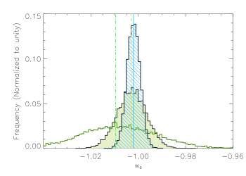
We first present our results for the magnitude case, as described in §3.1. The left panel of Figure 2 shows histograms of the best-fit values of from the likelihood analysis, after marginalizing over and . The empty histogram, which peaks at -1.009 (marked with a vertical dot-dashed line), is for the model with 300 SNe. The shaded histogram, representing the 2,000 SN case, peaks at -1.003 (vertical dashed line), while the hatched histogram representing the 10,000 SN case has its peak at -1.002 (vertical solid line). These distributions have 1 widths of 0.016, 0.006, and 0.003, respectively. This scatter is primarily due to the intrinsic uncertainty associated with absolute calibration, and is not dominated by lensing. Without the inclusion of lensing, however, the distributions peak at exactly -1, and show no bias. The shifted mode gives us a rough idea of the bias to be expected, on average, due to lensing. We find that 68% of the time a random sample of 300 SNe will have an estimated value for within 3% of its fiducial value, and this drops to 0.5% when a sample size of 10,000 SNe is considered.
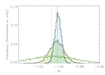
The right panel of Figure 2 shows the same distributions as the left panel, but this time using the flux-averaging technique instead of averaging over magnitudes. The empty, shaded, and hatched histograms peak at -1.007, -1.003, and -1.001, respectively, showing the mean bias for the 300, 2,000 and 10,000 SN cases (marked with dot-dashed, dashed, and solid vertical lines). With flux-averaging, we expect that 68% of the time a random sample of 300 SNe will yield a value of within 2.5% of the fiducial value, and within 0.5% for a sample of 10,000 SNe.
The 1 parameter uncertainty on ranges from the 20% level (for 300 SNe) to less than 5% (for 10,000 SNe), dwarfing the bias due to lensing. Thus, we need not be concerned about lensing degradation of dark energy parameter estimation for future JDEM-like surveys. We note, however, that our estimated bias on the EOS is larger than the lensing bias of quoted in Table 7 of Wood-Vasey et al. (2007). This is not surprising, given their use of the simple Gaussian approximation to lensing from Holz & Linder (2005), which is less effective for low statistics. Nonetheless, we agree with their conclusion that lensing is negligible. A similar conclusion was also reached by Martel & Premadi (2007) who used a compilation of 230 Type Ia SNe (Tonry et al., 2003) in the redshift range to show that the lensing errors are small compared to the intrinsic SNe errors.

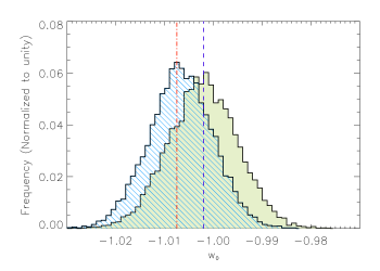
We now discuss the bias which arises if anomalous SNe are removed from the sample. Gravitational lensing causes some SNe to be highly magnified, and it is conceivable that these “obvious” outliers are subsequently removed from the analysis. In this case the mean of the sample will be shifted away from the true underlying Hubble diagram, and a bias will be introduced in the best-fit parameters. To quantify this effect, we remove SNe which deviate from the expected mean luminosity-distance relation in the Hubble diagram by more than 25% (corresponding roughly to a outlier). The SN scatter is a result of the convolution of the intrinsic error (Gaussian in flux of width 0.1) and the lensing PDF, and the outlier cutoff leads to a removal of 50 SNe out of the 2,000 SNe. These outliers are preferentially magnified, due to the strong lensing tail of the magnification distributions. The demagnification tail is cut off by the empty-beam lensing limit, and therefore isn’t as prominent. The hatched histogram in Figure 3 shows the distribution when events with convolved error greater than 2.5 are removed. The vertical dot-dashed line at -1.0075 shows the average value of obtained in this case, representing a bias in the estimate of roughly three times larger than when the full 2,000 SNe are analyzed (shown by shaded histogram). This bias is a result of cutting off the high magnification tail of the distribution, and thus shifting the data towards a net dimming of observed SNe, leading to a more negative value of .
We also apply a cutoff at , in addition to the discussed above. This results in a removal of SNe on average, for each 2,000 SN sample, and leads to a bias of %. Any arbitrary cut on the (non-Gaussian) convolved (lensing + intrinsic) sample leads to a net bias in the distance relation, and even for large outliers and large SN samples, this can lead to percent-level bias in the best-fit values for .
To summarize, we have quantified the effect of weak gravitational lensing on the estimation of dark energy EOS from type Ia supernova observations. With generated mock samples of 2,000 SNe distributed uniformly in redshift up to z1.7 (as expected in future surveys like JDEM), we have shown that the bias in parameter estimation due to lensing is less than 1 (which is well within the 1 uncertainty expected for these missions). Analyzing the data in flux or magnitude does not alter this result. If lensed supernovae that are highly magnified (such that the convolved error is more than 25% from the underlying Hubble diagram) are systematically removed from the sample, we find that the bias increases by a factor of almost three. Thus, so long as all observed SNe are used in the Hubble diagram, including ones that are highly magnified, the bias due to lensing in the estimate of the dark energy EOS will be significantly less than the 1 uncertainty. Even for a post-JDEM program with 10,000 SNe, lensing bias can be safely ignored.
References
- Aldering et al. (2004) Aldering, G. et al. 2004, PASP, submitted (astro-ph/0405232)
- Astier et al. (2006) Astier, P. et al., 2006, A & A, 447, 31
- Chevalier & Polarski (2001) M. Chevallier and D. Polarski, Int. J. Mod. Phys. D 10, 213 (2001).
- Cooray, Huterer, & Holz (2006) Cooray, A., Huterer, D., Holz, D. 2006, PRL, 96, 021301
- Frieman (1997) Frieman, J. A. 1997, Comments Astrophys., 18, 323
- Albrecht et al. (2006) Albrecht, A. et al. 2006, arXiv:astro-ph/0609591
- Holz & Linder (2005) Holz, D. E. & Linder, E. V. 2005, ApJ, 631, 678
- Holz & Wald (1998) Holz, D. E. & Wald, R. M. 1998, PRD, 58, 063501
- Hui & Greene (2006) Hui, L. & Greene, P. B. 2006, PRD, 73, 123526
- Huterer & Cooray (2005) Huterer, D. & Cooray, A. 2005, PRD, 71, 023506
- Knop et al. (2003) Knop, R. A. et al. 2003, ApJ, 598, 102
- Linder (2003) Linder, E. 2003, PRL, 90, 091301
- Martel & Premadi (2007) Martel, H. & Premadi, P. 2007, arXiv:0710.5452
- Perlmutter et al. (1999) Perlmutter, S., et al. 1999, ApJ, 517, 565
- Riess et al. (1998) Riess, A. G. et al. 1998, AJ, 116, 1009
- Riess et al. (2004) Riess, A. G. et al. 2004, ApJ, 607, 665
- Sereno, Piedipalumbo, & Sazhin (2002) Sereno, M., Piedipalumbo, E., Sazhin, M.V. 2002, MNRAS, 335, 1061
- Sullivan, Cooray, & Holz (2007) Sullivan, S., Cooray, A., & Holz, D. E. 2007, JCAP, 09, 004
- Sullivan et al. (2007) Sarkar, D., Sullivan, S., Joudaki, S., Amblard, A., Holz, D. E., & Cooray, A. 2007, arXiv:astro-ph/0709.1150
- Tonry et al. (2003) Tonry, J. L. et al. 2003, ApJ, 594, 1
- Wambsganss et al. (1997) Wambsganss, J., Cen, R., Xu, G., & Ostriker, J. P. 1997,ApJ, 475, L81
- Wang (2000) Wang, Y. 2000, ApJ, 536, 531
- Wang, Holz, & Munshi (2002) Wang, Y., Holz, D. E., Munshi, D. 2002, ApJ, 572, L15
- Wang & Mukherjee (2004) Wang, Y. & Mukherjee, P. 2004, ApJ, 606, 654
- Wood-Vasey et al. (2007) W. M. Wood-Vasey et al., arXiv:astro-ph/0701041.