On the Capacity Achieving Covariance Matrix for Rician MIMO Channels: An Asymptotic Approach

Résumé

In this contribution, the capacity-achieving input covariance matrices for coherent block-fading correlated MIMO Rician channels are determined. In contrast with the Rayleigh and uncorrelated Rician cases, no closed-form expressions for the eigenvectors of the optimum input covariance matrix are available. Classically, both the eigenvectors and eigenvalues are computed by numerical techniques. As the corresponding optimization algorithms are not very attractive, an approximation of the average mutual information is evaluated in this paper in the asymptotic regime where the number of transmit and receive antennas converge to $+\infty$ at the same rate. New results related to the accuracy of the corresponding large system approximation are provided. An attractive optimization algorithm of this approximation is proposed and we establish that it yields an effective way to compute the capacity achieving covariance matrix for the average mutual information. Finally, numerical simulation results show that, even for a moderate number of transmit and receive antennas, the new approach provides the same results as direct maximization approaches of the average mutual information, while being much more computationally attractive.

I Introduction

Since the seminal work of Telatar [39], the advantage of considering multiple antennas at the transmitter and the receiver in terms of capacity, for Gaussian and fast Rayleigh fading single-user channels, is well understood. In that paper, the figure of merit chosen for characterizing the performance of a coherent communication over a fading Multiple Input Multiple Output (MIMO) channel is the Ergodic Mutual Information (EMI). This choice will be justified in section II-C. Assuming the knowledge of the channel statistics at the transmitter, one important issue is then to maximize the EMI with respect to the channel input distribution. Without loss of optimality, the search for the optimal input distribution can be restricted to circularly Gaussian inputs. The problem then amounts to finding the optimum covariance matrix.

This optimization problem has been addressed extensively in the case of certain Rayleigh channels. In the context of the so-called Kronecker model, it has been shown by various authors (see e.g. [15] for a review) that the eigenvectors of the optimal input covariance matrix must coincide with the eigenvectors of the transmit correlation matrix. It is therefore sufficient to evaluate the eigenvalues of the optimal matrix, a problem which can be solved by using standard optimization algorithms. Note that [40] extended this result to more general (non Kronecker) Rayleigh channels.

Rician channels have been comparatively less studied from this point of view. Let us mention the work [19] devoted to the case of uncorrelated Rician channels, where the authors proved that the eigenvectors of the optimal input covariance matrix are the right-singular vectors of the line of sight component of the channel. As in the Rayleigh case, the eigenvalues can then be evaluated by standard routines. The case of correlated Rician channels is undoubtedly more complicated because the eigenvectors of the optimum matrix have no closed form expressions. Moreover, the exact expression of the EMI being complicated (see e.g. [22]), both the eigenvalues and the eigenvectors have to be evaluated numerically. In [42], a barrier interior-point method is proposed and implemented to directly evaluate the EMI as an expectation. The corresponding algorithms are however not very attractive because they rely on computationally-intensive Monte-Carlo simulations.

In this paper, we address the optimization of the input covariance of Rician channels with a two-sided (Kronecker) correlation. As the exact expression of the EMI is very complicated, we propose to evaluate an approximation of the EMI, valid when the number of transmit and receive antennas converge to $+\infty$ at the same rate, and then to optimize this asymptotic approximation. This will turn out to be a simpler problem. The results of the present contribution have been presented in part in the short conference paper [12].

The asymptotic approximation of the mutual information has been obtained by various authors in the case of MIMO Rayleigh channels, and has shown to be quite reliable even for a moderate number of antennas. The general case of a Rician correlated channel has recently been established in [17] using large random matrix theory and completes a number of previous works among which [9], [41] and [30] (Rayleigh channels), [8] and [31] (Rician uncorrelated channels), [10] (Rician receive correlated channel) and [37] (Rician correlated channels). Notice that the latest work (together with [30] and [31]) relies on the powerful but non-rigorous replica method. It also gives an expression for the variance of the mutual information. We finally mention the recent paper [38] in which the authors generalize our approach sketched in [12] to the MIMO Rician channel with interference. The optimization algorithm of the large system approximant of the EMI proposed in [38] is however different from our proposal.

In this paper, we rely on the results of [17] in which a closed-form asymptotic approximation for the mutual information is provided, and present new results concerning its accuracy. We then address the optimization of the large system approximation w.r.t. the input covariance matrix and propose a simple iterative maximization algorithm which, in some sense, can be seen as a generalization to the Rician case of [44] devoted to the Rayleigh context: Each iteration will be devoted to solve a system of two nonlinear equations as well as a standard waterfilling problem. Among the convergence results that we provide (and in contrast with [44]): We prove that the algorithm converges towards the optimum input covariance matrix as long as it converges. We also prove that the matrix which optimizes the large system approximation asymptotically achieves the capacity. This result has an important practical range as it asserts that the optimization algorithm yields a procedure that asymptotically achieves the true capacity. Finally, simulation results confirm the relevance of our approach.

The paper is organized as follows. Section II is devoted to the presentation of the channel model and the underlying assumptions. The asymptotic approximation of the ergodic mutual information is given in section III. In section IV, the strict concavity of the asymptotic approximation as a function of the covariance matrix of the input signal is established; it is also proved that the resulting optimal argument asymptotically achieves the true capacity. The maximization problem of the EMI approximation is studied in section V. Validations, interpretations and numerical results are provided in section VI.

II Problem statement

II-A General Notations

In this paper, the notations $s$, ${\bf x}$, $\mathbf{M}$ stand for scalars, vectors and matrices, respectively. As usual, $\|{\bf x}\|$ represents the Euclidian norm of vector ${\bf x}$ and $\|{\bf M}\|$ stands for the spectral norm of matrix ${\bf M}$. The superscripts $(.)^{T}$ and $(.)^{H}$ represent respectively the transpose and transpose conjugate. The trace of $\mathbf{M}$ is denoted by $\mathrm{Tr}(\mathbf{M})$. The mathematical expectation operator is denoted by $\mathbb{E}(\cdot)$ and the symbols $\Re$ and $\Im$ denote respectively the real and imaginary parts of a given complex number. If $x$ is a possibly complex-valued random variable, $\mathrm{Var}(x)=\mathbb{E}|x|^{2}-\left|\mathbb{E}(x)\right|^{2}$ represents the variance of $x$.

All along this paper, $r$ and $t$ stand for the number of transmit and receive antennas. Certain quantities will be studied in the asymptotic regime $t\rightarrow\infty$, $r\rightarrow\infty$ in such a way that ${\mathchoice{\dfrac{t}{r}}{\dfrac{t}{r}}{\frac{t}{r}}{\frac{t}{r}}}\rightarrow c\in(0,+\infty)$. In order to simplify the notations, $t\rightarrow+\infty$ should be understood from now on as $t\rightarrow\infty$, $r\rightarrow\infty$ and ${\mathchoice{\dfrac{t}{r}}{\dfrac{t}{r}}{\frac{t}{r}}{\frac{t}{r}}}\rightarrow c\in(0,+\infty)$. A matrix ${\bf M}_{t}$ whose size depends on $t$ is said to be uniformly bounded if $\sup_{t}\|{\bf M}_{t}\|<+\infty$.

Several variables used throughout this paper depend on various parameters, e.g. the number of antennas, the noise level, the covariance matrix of the transmitter, etc. In order to simplify the notations, we may not always mention all these dependencies.

II-B Channel model

We consider a wireless MIMO link with $t$ transmit and $r$ receive antennas. In our analysis, the channel matrix can possibly vary from symbol vector (or space-time codeword) to symbol vector. The channel matrix is assumed to be perfectly known at the receiver whereas the transmitter has only access to the statistics of the channel. The received signal can be written as

$${\bf y}(\tau)=\mathbf{H}(\tau){\bf x}(\tau)+{\bf z}(\tau)$$ (1)

where ${\bf x}(\tau)$ is the $t\times 1$ vector of transmitted symbols at time $\tau$, $\mathbf{H}(\tau)$ is the $r\times t$ channel matrix (stationary and ergodic process) and ${\bf z}(\tau)$ is a complex white Gaussian noise distributed as $N(0,\sigma^{2}\mathbf{I}_{r})$. For the sake of simplicity, we omit the time index $\tau$ from our notations. The channel input is subject to a power constraint $\mathrm{Tr}\left[\mathbb{E}({\bf x}{\bf x}^{H})\right]\leq t$. Matrix $\mathbf{H}$ has the following structure:

$$\mathbf{H}=\sqrt{\frac{K}{K+1}}{\bf A}+\frac{1}{\sqrt{K+1}}{\bf V}\ ,$$ (2)

where matrix $\bf{A}$ is deterministic, ${\bf V}$ is a random matrix and constant $K\geq 0$ is the so-called Rician factor which expresses the relative strength of the direct and scattered components of the received signal. Matrix $\bf{A}$ satisfies $\frac{1}{r}\mathrm{Tr}({\bf A}{\bf A}^{H})=1$ while ${\bf V}$ is given by

$${\bf V}={\mathchoice{\dfrac{1}{\sqrt{t}}}{\dfrac{1}{\sqrt{t}}}{\frac{1}{\sqrt{t}}}{\frac{1}{\sqrt{t}}}}\mathbf{C}^{{\mathchoice{\dfrac{1}{2}}{\dfrac{1}{2}}{\frac{1}{2}}{\frac{1}{2}}}}\mathbf{W}\mathbf{\tilde{C}}^{{\mathchoice{\dfrac{1}{2}}{\dfrac{1}{2}}{\frac{1}{2}}{\frac{1}{2}}}}\ ,$$ (3)

where $\mathbf{W}=(W_{ij})$ is a $r\times t$ matrix whose entries are independent and identically distributed (i.i.d.) complex circular Gaussian random variables ${\mathcal{C}N}(0,1)$, i.e. $W_{ij}=\Re W_{ij}+\mathbf{i}\Im W_{ij}$ where $\Re W_{ij}$ and $\Im W_{ij}$ are independent centered real Gaussian random variables with variance $\frac{1}{2}$. The matrices $\mathbf{\tilde{C}}>0$ and $\mathbf{C}>0$ account for the transmit and receive antenna correlation effects respectively and satisfy $\frac{1}{t}\mathrm{Tr}(\mathbf{\tilde{C}})=1$ and $\frac{1}{r}\mathrm{Tr}(\mathbf{C})=1$. This correlation structure is often referred to as a separable or Kronecker correlation model.

Remark 1

Note that no extra assumption related to the rank of the deterministic component ${\bf A}$ of the channel is done. Generally, it is often assumed that $\bf{A}$ has rank one ([15], [27], [18], [26], etc..) because of the relatively small path loss exponent of the direct path. Although the rank-one assumption is often relevant, it becomes questionable if one wants to address, for instance, a multi-user setup and determine the sum-capacity of a cooperative multiple access or broadcast channel in the high cooperation regime. Consider for example a macro-diversity situation in the downlink: Several base stations interconnected through ideal wireline channels cooperate to maximize the performance of a given multi-antenna receiver. Here the matrix ${\bf A}$ is likely to have a rank higher than one or even to be of full rank: Assume that the receive array of antennas is linear and uniform. Then a typical structure for ${\bf A}$ is

$${\bf A}={\mathchoice{\dfrac{1}{\sqrt{t}}}{\dfrac{1}{\sqrt{t}}}{\frac{1}{\sqrt{t}}}{\frac{1}{\sqrt{t}}}}\left[{\bf a}(\theta_{1}),\ldots,{\bf a}(\theta_{t})\right]{\boldsymbol{\Lambda}}\ ,$$ (4)

where ${\bf a}(\theta)=(1,e^{i\theta},\ldots,e^{i(r-1)\theta})^{T}$ and ${\bf\Lambda}$ is a diagonal matrix whose entries represent the complex amplitudes of the $t$ line of sight (LOS) components.

II-C Maximum ergodic mutual information

We denote by ${\cal C}$ the cone of nonnegative Hermitian $t\times t$ matrices and by ${\cal C}_{1}$ the subset of all matrices $\mathbf{Q}$ of ${\cal C}$ for which ${\mathchoice{\dfrac{1}{t}}{\dfrac{1}{t}}{\frac{1}{t}}{\frac{1}{t}}}\mbox{Tr}({\bf Q})=1$. Let $\mathbf{Q}$ be an element of ${\cal C}_{1}$ and denote by $I(\mathbf{Q})$ the ergodic mutual information (EMI) defined by:

$$I(\mathbf{Q})=\mathbb{E}_{\boldsymbol{H}}\left[\log\det\left({\bf I}_{r}+{\mathchoice{\dfrac{1}{\sigma^{2}}}{\dfrac{1}{\sigma^{2}}}{\frac{1}{\sigma^{2}}}{\frac{1}{\sigma^{2}}}}\mathbf{H}\mathbf{Q}\mathbf{H}^{H}\right)\right].$$ (5)

Maximizing the EMI with respect to the input covariance matrix $\mathbf{Q}=\mathbb{E}({\bf x}{\bf x}^{H})$ leads to the channel Shannon capacity for fast fading MIMO channels i.e. when the channel vary from symbol to symbol. This capacity is achieved by averaging over channel variations over time.

We will denote by $C_{E}$ the maximum value of the EMI over the set $\mathcal{C}_{1}$:

$$C_{E}=\sup_{\mathbf{Q}\in{\cal C}_{1}}I(\mathbf{Q}).$$ (6)

The optimal input covariance matrix thus coincides with the argument of the above maximization problem. Note that $I:\mathbf{Q}\mapsto I(\mathbf{Q})$ is a strictly concave function on the convex set ${\cal C}_{1}$, which guarantees the existence of a unique maximum ${\bf Q}_{*}$ (see [28]). When $\mathbf{\tilde{C}}=\mathbf{I}_{t}$, $\mathbf{C}=\mathbf{I}_{r}$, [19] shows that the eigenvectors of the optimal input covariance matrix coincide with the right-singular vectors of ${\bf A}$. By adapting the proof of [19], one can easily check that this result also holds when $\mathbf{\tilde{C}}=\mathbf{I}_{t}$ and ${\bf C}$ and ${\bf A}{\bf A}^{H}$ share a common eigenvector basis. Apart from these two simple cases, it seems difficult to find a closed-form expression for the eigenvectors of the optimal covariance matrix. Therefore the evaluation of $C_{E}$ requires the use of numerical techniques (see e.g. [42]) which are very demanding since they rely on computationally-intensive Monte-Carlo simulations. This problem can be circumvented as the EMI $I(\mathbf{Q})$ can be approximated by a simple expression denoted by $\bar{I}({\bf Q})$ (see section III) as $t\rightarrow\infty$ which in turn will be optimized with respect to ${\bf Q}$ (see section V).

Remark 2

Finding the optimum covariance matrix is useful in practice, in particular if the channel input is assumed to be Gaussian. In fact, there exist many practical space-time encoders that produce near-Gaussian outputs (these outputs are used as inputs for the linear precoder $\mathbf{Q}^{1/2}$). See for instance [34].

II-D Summary of the main results.

The main contributions of this paper can be summarized as follows:

1. We derive an accurate approximation of $I({\bf Q})$ as $t\rightarrow+\infty$: $I({\bf Q})\simeq\bar{I}({\bf Q})$ where

   $$\bar{I}({\bf Q})=\log\mathrm{det}\left[{\bf I}_{t}+{\bf G}(\delta({\bf Q},\tilde{\delta}({\bf Q})){\bf Q}\right]+i(\delta({\bf Q}),\tilde{\delta}({\bf Q}))$$ (7)

   where $\delta({\bf Q})$ and $\tilde{\delta}({\bf Q})$ are two positive terms defined as the solutions of a system of 2 equations (see Eq. (33)). The functions ${\bf G}$ and $i$ depend on $(\delta({\bf Q}),\tilde{\delta}({\bf Q}))$, $K$, ${\bf A}$, ${\bf C}$, $\tilde{{\bf C}}$, and on the noise variance $\sigma^{2}$. They are given in closed form.

   The derivation of $\bar{I}({\bf Q})$ is based on the observation that the eigenvalue distribution of random matrix ${\bf H}{\bf Q}{\bf H}^{H}$ becomes close to a deterministic distribution as $t\rightarrow+\infty$. This in particular implies that if $(\lambda_{i})_{1\leq i\leq r}$ represent the eigenvalues of ${\bf H}{\bf Q}{\bf H}^{H}$, then:

   $$\frac{1}{r}\log\mathrm{det}\left[{\bf I}_{r}+{\mathchoice{\dfrac{1}{\sigma^{2}}}{\dfrac{1}{\sigma^{2}}}{\frac{1}{\sigma^{2}}}{\frac{1}{\sigma^{2}}}}\mathbf{H}\mathbf{Q}\mathbf{H}^{H}\right]=\frac{1}{r}\sum_{i=1}^{r}\log\left(1+\frac{\lambda_{i}}{\sigma^{2}}\right)$$

   has the same behaviour as a deterministic term, which turns out to be equal to $\frac{\bar{I}({\bf Q})}{r}$. Taking the mathematical expectation w.r.t. the distribution of the channel, and multiplying by $r$ gives $I({\bf Q})\simeq\bar{I}({\bf Q})$.

   The error term $I({\bf Q})-\bar{I}({\bf Q})$ is shown to be of order $O(\frac{1}{t})$. As $I({\bf Q})$ is known to increase linearly with $t$, the relative error $\frac{I({\bf Q})-\bar{I}({\bf Q})}{I({\bf Q})}$ is of order $O(\frac{1}{t^{2}})$. This supports the fact that $\bar{I}({\bf Q})$ is an accurate approximation of $I({\bf Q})$, and that it is relevant to study $\bar{I}({\bf Q})$ in order to obtain some insight on $I({\bf Q})$.

2. We prove that the function ${\bf Q}\mapsto\bar{I}({\bf Q})$ is strictly concave on ${\cal C}_{1}$. As a consequence, the maximum of $\bar{I}$ over ${\cal C}_{1}$ is reached for a unique matrix $\overline{\bf Q}_{*}$. We also show that $I(\overline{\bf Q}_{*})-I({\bf Q}_{*})=O(1/t)$ where we recall that ${\bf Q}_{*}$ is the capacity achieving covariance matrix. Otherwise stated, the computation of $\overline{\bf Q}_{*}$ (see below) allows one to (asymptotically) achieve the capacity $I({\bf Q}_{*})$.

3. We study the structure of $\overline{\bf Q}_{*}$ and establish that $\overline{\bf Q}_{*}$ is solution of the standard waterfilling problem:

   $$\max_{{\bf Q}\in{\cal C}_{1}}\log\mathrm{det}\left({\bf I}+{\bf G}(\delta_{*},\tilde{\delta}_{*}){\bf Q}\right)\ ,$$

   where $\delta_{*}=\delta(\overline{\bf Q}_{*})$, $\tilde{\delta}_{*}=\tilde{\delta}(\overline{\bf Q}_{*})$ and

   $${\bf G}(\delta_{*},\tilde{\delta}_{*})=\frac{\delta_{*}}{K+1}\tilde{{\bf C}}+\frac{1}{\sigma^{2}}\frac{K}{K+1}{\bf A}^{H}\left({\bf I}_{r}+\frac{\tilde{\delta}_{*}}{K+1}\,{\bf C}\right)^{-1}{\bf A}\ .$$

   This result provides insights on the structure of the approximating capacity achieving covariance matrix, but cannot be used to evaluate $\overline{\bf Q}_{*}$ since the parameters $\delta_{*}$ and $\tilde{\delta}_{*}$ depend on the optimum matrix $\overline{\bf Q}_{*}$. We therefore propose an attractive iterative maximization algorithm of $\bar{I}({\bf Q})$ where each iteration consists in solving a standard waterfilling problem and a $2\times 2$ system characterizing the parameters $(\delta,\tilde{\delta})$.

III Asymptotic behavior of the ergodic mutual information

In this section, the input covariance matrix $\mathbf{Q}\in{\cal C}_{1}$ is fixed and the purpose is to evaluate the asymptotic behaviour of the ergodic mutual information $I(\mathbf{Q})$ as $t\rightarrow\infty$ (recall that $t\rightarrow+\infty$ means $t\rightarrow\infty$, $r\rightarrow\infty$ and $t/r\rightarrow c\in(0,+\infty)$).

As we shall see, it is possible to evaluate in closed form an accurate approximation $\bar{I}({\bf Q})$ of $I(\mathbf{Q})$. The corresponding result is partly based on the results of [17] devoted to the study of the asymptotic behaviour of the eigenvalue distribution of matrix $\boldsymbol{\Sigma}\boldsymbol{\Sigma}^{H}$ where $\boldsymbol{\Sigma}$ is given by

$$\boldsymbol{\Sigma}={\bf B}+{\bf Y}\ ,$$ (8)

matrix ${\bf B}$ being a deterministic $r\times t$ matrix, and ${\bf Y}$ being a $r\times t$ zero mean (possibly complex circular Gaussian) random matrix with independent entries whose variance is given by $\mathrm{E}|Y_{ij}|^{2}=\frac{\sigma^{2}_{ij}}{t}$. Notice in particular that the variables $(Y_{ij};\ 1\leq i\leq r,\ 1\leq j\leq t)$ are not necessarily identically distributed. We shall refer to the triangular array $(\sigma^{2}_{ij};\ 1\leq i\leq r,\ 1\leq j\leq t)$ as the variance profile of $\boldsymbol{\Sigma}$; we shall say that it is separable if $\sigma^{2}_{ij}=d_{i}\tilde{d}_{j}$ where $d_{i}\geq 0$ for $1\leq i\leq r$ and $\tilde{d}_{j}\geq 0$ for $1\leq j\leq t$. Due to the unitary invariance of the EMI of Gaussian channels, the study of $I(\mathbf{Q})$ will turn out to be equivalent to the study of the EMI of model (8) in the complex circular Gaussian case with a separable variance profile.

III-A Study of the EMI of the equivalent model (8).

We first introduce the resolvent and the Stieltjes transform associated with ${\bf\Sigma\Sigma}^{H}$ (Section III-A1); we then introduce auxiliary quantities (Section III-A2) and their main properties; we finally introduce the approximation of the EMI in this case (Section III-A3).

III-A1 The resolvent, the Stieltjes transform

Denote by ${\bf S}(\sigma^{2})$ and $\tilde{{\bf S}}(\sigma^{2})$ the resolvents of matrices $\boldsymbol{\Sigma}\boldsymbol{\Sigma}^{H}$ and $\boldsymbol{\Sigma}^{H}\boldsymbol{\Sigma}$ defined by:

$${\bf S}(\sigma^{2})=\left[\boldsymbol{\Sigma}\boldsymbol{\Sigma}^{H}+\sigma^{2}{\bf I}_{r}\right]^{-1},\qquad\tilde{{\bf S}}(\sigma^{2})=\left[\boldsymbol{\Sigma}^{H}\boldsymbol{\Sigma}+\sigma^{2}{\bf I}_{t}\right]^{-1}\ .$$ (9)

These resolvents satisfy the obvious, but useful property:

$${\bf S}(\sigma^{2})\leq\frac{{\bf I}_{r}}{\sigma^{2}},\qquad\tilde{{\bf S}}(\sigma^{2})\leq\frac{{\bf I}_{t}}{\sigma^{2}}\ .$$ (10)

Recall that the Stieltjes transform of a nonnegative measure $\mu$ is defined by $\int\frac{\mu(d\lambda)}{\lambda-z}$. The quantity $s(\sigma^{2})=\frac{1}{r}\mathrm{Tr}({\bf S}(\sigma^{2}))$ coincides with the Stieltjes transform of the eigenvalue distribution of matrix $\boldsymbol{\Sigma}\boldsymbol{\Sigma}^{H}$ evaluated at point $z=-\sigma^{2}$. In fact, denote by $(\lambda_{i})_{1\leq i\leq r}$ its eigenvalues , then:

$$s(\sigma^{2})=\frac{1}{r}\sum_{i=1}^{r}\frac{1}{\lambda_{i}+\sigma^{2}}=\int_{\mathrm{R}^{+}}\frac{\nu(d\lambda)}{\lambda+\sigma^{2}}\ ,$$

where $\nu$ represents the eigenvalue distribution of $\boldsymbol{\Sigma}\boldsymbol{\Sigma}^{H}$ defined as the probability distribution:

$$\nu=\frac{1}{r}\sum_{i=1}^{r}\delta_{\lambda_{i}}$$

where $\delta_{x}$ represents the Dirac distribution at point $x$. The Stieltjes transform $s(\sigma^{2})$ is important as the characterization of the asymptotic behaviour of the eigenvalue distribution of $\boldsymbol{\Sigma}\boldsymbol{\Sigma}^{H}$ is equivalent to the study of $s(\sigma^{2})$ when $t\rightarrow+\infty$ for each $\sigma^{2}$. This observation is the starting point of the approaches developed by Pastur [29], Girko [13], Bai and Silverstein [1], etc.

We finally recall that a positive $p\times p$ matrix-valued measure $\boldsymbol{\mu}$ is a function defined on the Borel subsets of $\mathbb{R}$ onto the set of all complex-valued $p\times p$ matrices satisfying:

• For each Borel set $B$, $\boldsymbol{\mu}(B)$ is a Hermitian nonnegative definite $p\times p$ matrix with complex entries;

• $\boldsymbol{\mu}(0)={\bf 0}$;

• For each countable family $(B_{n})_{n\in\mathrm{N}}$ of disjoint Borel subsets of $\mathrm{R}$,

  $$\boldsymbol{\mu}(\cup_{n}B_{n})=\sum_{n}\boldsymbol{\mu}(B_{n})\ .$$

Note that for any nonnegative Hermitian $p\times p$ matrix ${\bf M}$, then $\mathrm{Tr}({\bf M}\boldsymbol{\mu})$ is a (scalar) positive measure. The matrix-valued measure $\boldsymbol{\mu}$ is said to be finite if $\mathrm{Tr}(\boldsymbol{\mu}(\mathbb{R}))<+\infty$.

III-A2 The auxiliary quantities $\beta,\tilde{\beta}$, ${\bf T}$ and ${\bf\tilde{T}}$

We gather in this section many results of [17] that will be of help in the sequel.

Assumption 1

Let $({\bf B}_{t})$ be a family of $r\times t$ deterministic matrices such that: $\sup_{t,i}\sum_{j=1}^{t}|B_{ij}|^{2}<+\infty,\;\sup_{t,j}\sum_{i=1}^{r}|B_{ij}|^{2}<+\infty$ .

Theorem 1

Recall that ${\bf\Sigma}={\bf B}+{\bf Y}$ and assume that ${\bf Y}=\frac{1}{\sqrt{t}}{\bf D}^{\frac{1}{2}}{\bf X}\,\tilde{{\bf D}}^{\frac{1}{2}}$, where ${\bf D}$ and $\tilde{{\bf D}}$ represent the diagonal matrices ${\bf D}=\mbox{diag}(d_{i},\,1\leq i\leq r)$ and $\tilde{{\bf D}}=\mbox{diag}(\tilde{d}_{j},\ 1\leq j\leq t)$ respectively, and where ${\bf X}$ is a matrix whose entries are i.i.d. complex centered with variance one. The following facts hold true:

• (Existence and uniqueness of auxiliary quantities) For $\sigma^{2}$ fixed, consider the system of equations:

  $$\left\{\begin{array}[]{l}\beta=\displaystyle{\frac{1}{t}\textrm{Tr}\left[{\bf D}\left(\sigma^{2}({\bf I}_{r}+{\bf D}\tilde{\beta})+{\bf B}({\bf I}_{t}+\tilde{{\bf D}}\beta)^{-1}{\bf B}^{H}\right)^{-1}\right]}\\ \tilde{\beta}=\displaystyle{\frac{1}{t}\textrm{Tr}\left[\tilde{{\bf D}}\left(\sigma^{2}({\bf I}_{t}+\tilde{{\bf D}}\beta)+{\bf B}^{H}({\bf I}_{r}+{\bf D}\tilde{\beta})^{-1}{\bf B}\right)^{-1}\right]}\end{array}\right..$$ (11)

  Then, the system (11) admits a unique couple of positive solutions $(\beta(\sigma^{2}),\tilde{\beta}(\sigma^{2}))$. Denote by ${\bf T}(\sigma^{2})$ and $\tilde{{\bf T}}(\sigma^{2})$ the following matrix-valued functions:

  $$\left\{\begin{array}[]{ccc}{\bf T}(\sigma^{2})&=&\left[\sigma^{2}({\bf I}+\tilde{\beta}(\sigma^{2}){\bf D})+{\bf B}({\bf I}+\beta(\sigma^{2})\tilde{{\bf D}})^{-1}{\bf B}^{H}\right]^{-1}\\ \tilde{{\bf T}}(\sigma^{2})&=&\left[\sigma^{2}({\bf I}+\beta(\sigma^{2})\tilde{{\bf D}})+{\bf B}^{H}({\bf I}+\tilde{\beta}(\sigma^{2}){\bf D})^{-1}{\bf B}\right]^{-1}\end{array}\right.\ .$$ (12)

  Matrices ${\bf T}(\sigma^{2})$ and $\tilde{{\bf T}}(\sigma^{2})$ satisfy

  $${\bf T}(\sigma^{2})\leq\frac{{\bf I}_{r}}{\sigma^{2}},\qquad\tilde{{\bf T}}(\sigma^{2})\leq\frac{{\bf I}_{t}}{\sigma^{2}}\ .$$ (13)

• (Representation of the auxiliary quantities) There exist two uniquely defined positive matrix-valued measures $\boldsymbol{\mu}$ and $\tilde{\boldsymbol{\mu}}$ such that $\boldsymbol{\mu}(\mathbb{R}^{+})={\bf I}_{r}$, $\tilde{\boldsymbol{\mu}}(\mathbb{R}^{+})={\bf I}_{t}$ and

  $${\bf T}(\sigma^{2})=\int_{\mathrm{R}^{+}}\frac{\boldsymbol{\mu}(d\lambda)}{\lambda+\sigma^{2}},\qquad\tilde{{\bf T}}(\sigma^{2})=\int_{\mathrm{R}^{+}}\frac{\tilde{\boldsymbol{\mu}}(d\lambda)}{\lambda+\sigma^{2}}\ .$$ (14)

  The solutions $\beta(\sigma^{2})$ and $\tilde{\beta}(\sigma^{2})$ of system (11) are given by:

  $$\beta(\sigma^{2})=\frac{1}{t}\mathrm{Tr}{\bf D}{\bf T}(\sigma^{2})\ ,\qquad\tilde{\beta}(\sigma^{2})=\frac{1}{t}\mathrm{Tr}\tilde{{\bf D}}\tilde{{\bf T}}(\sigma^{2})\ ,$$ (15)

  and can thus be written as

  $$\beta(\sigma^{2})=\int_{\mathrm{R}^{+}}\frac{\mu_{b}(d\lambda)}{\lambda+\sigma^{2}}\ ,\qquad\tilde{\beta}(\sigma^{2})=\int_{\mathrm{R}^{+}}\frac{\tilde{\mu}_{b}(d\lambda)}{\lambda+\sigma^{2}}$$ (16)

  where $\mu_{b}$ and $\tilde{\mu}_{b}$ are nonnegative scalar measures defined by

  $$\mu_{b}(d\lambda)=\frac{1}{t}\mathrm{Tr}({\bf D}\boldsymbol{\mu}(d\lambda))\quad\textrm{and}\quad\tilde{\mu}_{b}(d\lambda)=\frac{1}{t}\mathrm{Tr}(\tilde{{\bf D}}\tilde{\boldsymbol{\mu}}(d\lambda)).$$

• (Asymptotic approximation) Assume that Assumption 1 holds and that

  $$\sup_{t}\|{\bf D}\|<d_{\max}<+\infty\quad\textrm{and}\quad\sup_{t}\|\tilde{{\bf D}}\|<\tilde{d}_{\max}<+\infty\ .$$

  For every deterministic matrices ${\bf M}$ and $\tilde{{\bf M}}$ satisfying $\sup_{t}\|{\bf M}\|<+\infty$ and $\sup_{t}\|\tilde{{\bf M}}\|<+\infty$, the following limits hold true almost surely:

  $$\left\{\begin{array}[]{ccc}\lim_{t\rightarrow+\infty}\frac{1}{r}\mathrm{Tr}\left[({\bf S}(\sigma^{2})-{\bf T}(\sigma^{2})){\bf M}\right]&=&0\\ \lim_{t\rightarrow+\infty}\frac{1}{t}\mathrm{Tr}\left[(\tilde{{\bf S}}(\sigma^{2})-\tilde{{\bf T}}(\sigma^{2}))\tilde{{\bf M}}\right]&=&0\end{array}\right.\ .$$ (17)

  Denote by $\mu$ and $\tilde{\mu}$ the (scalar) probability measures $\mu=\frac{1}{r}\mathrm{Tr}\boldsymbol{\mu}$ and $\tilde{\mu}=\frac{1}{t}\mathrm{Tr}\tilde{\boldsymbol{\mu}}$, by $(\lambda_{i})$ (resp. $(\tilde{\lambda}_{j})$) the eigenvalues of $\boldsymbol{\Sigma}\boldsymbol{\Sigma}^{H}$ (resp. of $\boldsymbol{\Sigma}^{H}\boldsymbol{\Sigma}$). The following limits hold true almost surely:

  $$\left\{\begin{array}[]{ccc}\lim_{t\rightarrow+\infty}\frac{1}{r}\sum_{i=1}^{r}\phi(\lambda_{i})-\int_{0}^{+\infty}\phi(\lambda)\;\mu(d\lambda)&=&0\\ \lim_{t\rightarrow+\infty}\frac{1}{t}\sum_{j=1}^{t}\tilde{\phi}(\lambda_{j})-\int_{0}^{+\infty}\tilde{\phi}(\lambda)\;\tilde{\mu}(d\lambda)&=&0\end{array}\right.\ ,$$ (18)

  for continuous bounded functions $\phi$ and $\tilde{\phi}$ defined on $\mathbb{R}^{+}$.

The proof of $(i)$ is provided in Appendix A (note that in [17], the existence and uniqueness of solutions to the system (11) is proved in a certain class of analytic functions depending on $\sigma^{2}$ but this does not imply the existence of a unique solution $(\beta,\tilde{\beta})$ when $\sigma^{2}$ is fixed). The rest of the statements of Theorem 1 have been established in [17], and their proof is omitted here.

Remark 3

As shown in [17], the results in Theorem 1 do not require any Gaussian assumption for $\boldsymbol{\Sigma}$. Remark that (17) implies in some sense that the entries of ${\bf S}(\sigma^{2})$ and $\tilde{{\bf S}}(\sigma^{2})$ have the same behaviour as the entries of the deterministic matrices ${\bf T}(\sigma^{2})$ and $\tilde{{\bf T}}(\sigma^{2})$ (which can be evaluated by solving the system (11)). In particular, using (17) for ${\bf M}={\bf I}$, it follows that the Stieltjes transform $s(\sigma^{2})$ of the eigenvalue distribution of $\boldsymbol{\Sigma}\boldsymbol{\Sigma}^{H}$ behaves like $\frac{1}{r}\mathrm{Tr}{\bf T}(\sigma^{2})$, which is itself the Stieltjes transform of measure $\mu=\frac{1}{r}\mathrm{Tr}\boldsymbol{\mu}$. The convergence statement (18) which states that the eigenvalue distribution of $\boldsymbol{\Sigma}\boldsymbol{\Sigma}^{H}$ (resp. $\boldsymbol{\Sigma}^{H}\boldsymbol{\Sigma}$) has the same behavior as $\mu$ (resp. $\tilde{\mu}$) directly follows from this observation.

III-A3 The asymptotic approximation of the EMI

Denote by $J(\sigma^{2})=\mathbb{E}\log\det\left({\bf I}_{r}+\sigma^{-2}\boldsymbol{\Sigma}\boldsymbol{\Sigma}^{H}\right)$ the EMI associated with matrix ${\bf\Sigma}$. First notice that

$$\log\det\left({\bf I}+\frac{\boldsymbol{\Sigma}\boldsymbol{\Sigma}^{H}}{\sigma^{2}}\right)=\sum_{i=1}^{r}\log\left(1+\frac{\lambda_{i}}{\sigma^{2}}\right)\ ,$$

where the $\lambda_{i}$’s stand for the eigenvalues of $\boldsymbol{\Sigma}\boldsymbol{\Sigma}^{H}$. Applying (18) to function $\phi(\lambda)=\log(\lambda+\sigma^{2})$ (plus some extra work since $\phi$ is not bounded), we obtain:

$$\lim_{t\rightarrow+\infty}\left(\frac{1}{r}\log\det\left({\bf I}+\frac{\boldsymbol{\Sigma}\boldsymbol{\Sigma}^{H}}{\sigma^{2}}\right)-\int_{0}^{+\infty}\log(\lambda+\sigma^{2})\;d\mu(\lambda)\right)=0\ .$$ (19)

Using the well known relation:

$$\frac{1}{r}\log\det\left({\bf I}+\frac{\boldsymbol{\Sigma}\boldsymbol{\Sigma}^{H}}{\sigma^{2}}\right) = \int_{\sigma^{2}}^{+\infty}\left(\frac{1}{\omega}-\frac{1}{r}\mathrm{Tr}(\boldsymbol{\Sigma}\boldsymbol{\Sigma}^{H}+\omega{\bf I})^{-1}\right)\;d\omega$$ (20)

$$= \int_{\sigma^{2}}^{+\infty}\left(\frac{1}{\omega}-\frac{1}{r}\mathrm{Tr}\,{\bf S}(\omega)\right)\;d\omega\ ,$$

together with the fact that ${\boldsymbol{S}}(\omega)\approx{\boldsymbol{T}}(\omega)$ (which follows from Theorem 1), it is proved in [17] that:

$$\lim_{t\rightarrow+\infty}\left[\frac{1}{r}\log\det\left({\bf I}+\frac{\boldsymbol{\Sigma}\boldsymbol{\Sigma}^{H}}{\sigma^{2}}\right)-\int_{\sigma^{2}}^{+\infty}\left(\frac{1}{\omega}-\frac{1}{r}\mathrm{Tr}{\bf T}(\omega)\right)\;d\omega\right]=0$$ (21)

almost surely. Define by $\bar{J}(\sigma^{2})$ the quantity:

$$\bar{J}(\sigma^{2})=r\int_{\sigma^{2}}^{+\infty}\left(\frac{1}{\omega}-\frac{1}{r}\mathrm{Tr}{\bf T}(\omega)\right)\;d\omega\ .$$ (22)

Then, $\bar{J}(\sigma^{2})$ can be expressed more explicitely as:

$$\bar{J}(\sigma^{2})=\log\det\left[{\bf I}_{r}+\tilde{\beta}(\sigma^{2}){\bf D}+\frac{1}{\sigma^{2}}{\bf B}({\bf I}_{t}+\beta(\sigma^{2})\tilde{{\bf D}})^{-1}{\bf B}^{H}\right]\\ +\log\det\left[{\bf I}_{t}+\beta(\sigma^{2})\tilde{{\bf D}}\right]-\sigma^{2}t\beta(\sigma^{2})\tilde{\beta}(\sigma^{2})\ ,$$ (23)

or equivalently as

$$\bar{J}(\sigma^{2})=\log\det\left[{\bf I}_{t}+\beta(\sigma^{2})\tilde{{\bf D}}+\frac{1}{\sigma^{2}}{\bf B}^{H}({\bf I}_{r}+\tilde{\beta}(\sigma^{2}){\bf D})^{-1}{\bf B}\right]\\ +\log\det\left[{\bf I}_{r}+\tilde{\beta}(\sigma^{2}){\bf D}\right]-\sigma^{2}t\beta(\sigma^{2})\tilde{\beta}(\sigma^{2})\ .$$ (24)

Taking the expectation with respect to the channel $\boldsymbol{\Sigma}$ in (21), the EMI $J(\sigma^{2})=\mathbb{E}\log\det\left({\bf I}_{r}+\sigma^{-2}\boldsymbol{\Sigma}\boldsymbol{\Sigma}^{H}\right)$ can be approximated by $\bar{J}(\sigma^{2})$:

$$J(\sigma^{2})=\bar{J}(\sigma^{2})+o(t)$$ (25)

as $t\rightarrow+\infty$. This result is fully proved in [17] and is of potential interest since the numerical evaluation of $\bar{J}(\sigma^{2})$ only requires to solve the $2\times 2$ system (11) while the calculation of $J(\sigma^{2})$ either rely on Monte-Carlo simulations or on the implementation of rather complicated explicit formulas (see for instance [22]).

In order to evaluate the precision of the asymptotic approximation $\bar{J}$, we shall improve (25) and get the speed $J(\sigma^{2})=\bar{J}(\sigma^{2})+O(t^{-1})$ in the next theorem. This result completes those in [17] and on the contrary of the rest of Theorem 1 heavily relies on the Gaussian structure of ${\bf\Sigma}$. We first introduce very mild extra assumptions:

Assumption 2

Let $({\bf B}_{t})$ be a family of $r\times t$ deterministic matrices such that

$$\sup_{t}\|{\bf B}\|<b_{\max}<+\infty\ .$$

Assumption 3

Let ${\bf D}$ and $\tilde{{\bf D}}$ be respectively $r\times r$ and $t\times t$ diagonal matrices such that

$$\sup_{t}\|{\bf D}\|<d_{\max}<+\infty\quad\textrm{and}\quad\sup_{t}\|\tilde{{\bf D}}\|<\tilde{d}_{\max}<+\infty\ .$$

Assume moreover that

$$\inf_{t}\frac{1}{t}\mathrm{Tr}{\bf D}>0\quad\textrm{and}\quad\inf_{t}\frac{1}{t}\mathrm{Tr}\tilde{{\bf D}}>0\ .$$

Theorem 2

Recall that ${\bf\Sigma}={\bf B}+{\bf Y}$ and assume that ${\bf Y}=\frac{1}{\sqrt{t}}{\bf D}^{\frac{1}{2}}{\bf X}\,\tilde{{\bf D}}^{\frac{1}{2}}$, where ${\bf D}=\mbox{diag}(d_{i})$ and $\tilde{{\bf D}}=\mbox{diag}(\tilde{d}_{j})$ are $r\times r$ and $t\times t$ diagonal matrices and where ${\bf X}$ is a matrix whose entries are i.i.d. complex circular Gaussian variables ${\mathcal{C}N}(0,1)$. Assume moreover that Assumptions 2 and 3 hold true. Then, for every deterministic matrices ${\bf M}$ and $\tilde{{\bf M}}$ satisfying $\sup_{t}\|{\bf M}\|<+\infty$ and $\sup_{t}\|\tilde{{\bf M}}\|<+\infty$, the following facts hold true:

$$\mathrm{Var}\,\left(\frac{1}{r}\mathrm{Tr}\left[{\bf S}(\sigma^{2}){\bf M}\right]\right)=O\left(\frac{1}{t^{2}}\right)\quad\textrm{and}\quad\mathrm{Var}\,\left(\frac{1}{t}\mathrm{Tr}\left[\tilde{{\bf S}}(\sigma^{2})\tilde{{\bf M}}\right]\right)=O\left(\frac{1}{t^{2}}\right)$$ (26)

where $\mathrm{Var}(.)$ stands for the variance. Moreover,

$$\begin{array}[]{ccc}\frac{1}{r}\mathrm{Tr}\left[(\mathbb{E}({\bf S}(\sigma^{2}))-{\bf T}(\sigma^{2})){\bf M}\right]&=&O\left(\frac{1}{t^{2}}\right)\\ \frac{1}{t}\mathrm{Tr}\left[(\mathbb{E}(\tilde{{\bf S}}(\sigma^{2}))-\tilde{{\bf T}}(\sigma^{2}))\tilde{{\bf M}}\right]&=&O\left(\frac{1}{t^{2}}\right)\end{array}$$ (27)

and

$$J(\sigma^{2})=\bar{J}(\sigma^{2})+O\left(\frac{1}{t}\right)\ .$$ (28)

The proof is given in Appendix B. We provide here some comments.

Remark 4

The proof of Theorem 2 takes full advantage of the Gaussian structure of matrix $\boldsymbol{\Sigma}$ and relies on two simple ingredients:

• An integration by parts formula that provides an expression for the expectation of certain functionals of Gaussian vectors, already well-known and widely used in Random Matrix Theory [25, 32].

• An inequality known as Poincaré-Nash inequality that bounds the variance of functionals of Gaussian vectors. Although well known, its application to random matrices is fairly recent ([6], [33], see also [16]).

Remark 5

Equations (26) also hold in the non Gaussian case and can be established by using the so-called REFORM (Resolvent FORmula Martingale) method introduced by Girko ([13]).

Equations (27) and (28) are specific to the complex Gaussian structure of the channel matrix $\boldsymbol{\Sigma}$. In particular, in the non Gaussian case, or in the real Gaussian case, one would get $J(\sigma^{2})=\bar{J}(\sigma^{2})+O(1)$. These two facts are in accordance with:

• The work of [2] in which a weaker result ($o(1)$ instead of $O(t^{-1})$) is proved in the simpler case where ${\bf B}={\bf 0}$;

• The predictions of the replica method in [30] (resp. [31]) in the case where ${\bf B}=\mathbf{0}$ (resp. in the case where $\mathbf{\tilde{D}}=\mathbf{I}_{t}$ and ${\bf D}={\bf I}_{r}$);

Remark 6 (Standard deviation and bias)

Eq. (26) implies that the standard deviation of $\frac{1}{r}\mathrm{Tr}\left[({\bf S}(\sigma^{2})-{\bf T}(\sigma^{2})){\bf M}\right]$ and $\frac{1}{t}\mathrm{Tr}\left[(\tilde{{\bf S}}(\sigma^{2})-\tilde{{\bf T}}(\sigma^{2}))\tilde{{\bf M}}\right]$ are of order $O(t^{-1})$ terms. However, their mathematical expectations (which correspond to the bias) converge much faster towards $0$ as (27) shows (the order is $O(t^{-2})$).

Remark 7

By adapting the techniques developed in the course of the proof of Theorem 2, one may establish that ${\bf u}^{H}\mathbb{E}{\bf S}(\sigma^{2}){\bf v}-{\bf u}^{H}{\bf T}(\sigma^{2}){\bf v}=O\left(\frac{1}{t}\right)\ ,$ where ${\bf u}$ and ${\bf v}$ are uniformly bounded $r$-dimensional vectors.

Remark 8

Both $J(\sigma^{2})$ and $\bar{J}(\sigma^{2})$ increase linearly with $t$. Equation (28) thus implies that the relative error $\frac{J(\sigma^{2})-\bar{J}(\sigma^{2})}{J(\sigma^{2})}$ is of order $O(t^{-2})$. This remarkable convergence rate strongly supports the observed fact that approximations of the EMI remain reliable even for small numbers of antennas (see also the numerical results in section VI). Note that similar observations have been done in other contexts where random matrices are used, see e.g. [3], [30].

III-B Introduction of the virtual channel ${\bf HQ}^{\frac{1}{2}}$

The purpose of this section is to establish a link between the simplified model (8): ${\bf\Sigma}={\bf B}+{\bf Y}$ where ${\bf Y}=\frac{1}{\sqrt{t}}{\bf D}^{\frac{1}{2}}{\bf X}\tilde{\bf D}^{\frac{1}{2}}$, ${\bf X}$ being a matrix with i.i.d ${\mathcal{C}}N(0,1)$ entries, ${\bf D}$ and $\tilde{\bf D}$ being diagonal matrices, and the Rician model (2) under investigation: $\mathbf{H}=\sqrt{\frac{K}{K+1}}{\bf A}+\frac{1}{\sqrt{K+1}}{\bf V}$ where ${\bf V}=\frac{1}{\sqrt{t}}{\bf C}^{\frac{1}{2}}{\bf W}\tilde{\bf C}^{\frac{1}{2}}$. As we shall see, the key point is the unitary invariance of the EMI of Gaussian channels together with a well-chosen eingenvalue/eigenvector decomposition.

We introduce the virtual channel ${\bf H}{\bf Q}^{{\mathchoice{\dfrac{1}{2}}{\dfrac{1}{2}}{\frac{1}{2}}{\frac{1}{2}}}}$ which can be written as:

$${\bf H}{\bf Q}^{\frac{1}{2}}=\sqrt{\frac{K}{K+1}}{\bf A}{\bf Q}^{\frac{1}{2}}+\frac{1}{\sqrt{K+1}}{\bf C}^{\frac{1}{2}}\frac{{\bf W}}{\sqrt{t}}\boldsymbol{\Theta}({\bf Q}^{\frac{1}{2}}\tilde{{\bf C}}{\bf Q}^{\frac{1}{2}})^{\frac{1}{2}}\ ,$$ (29)

where $\boldsymbol{\Theta}$ is the deterministic unitary $t\times t$ matrix defined by

$$\boldsymbol{\Theta}=\tilde{{\bf C}}^{\frac{1}{2}}{\bf Q}^{\frac{1}{2}}({\bf Q}^{\frac{1}{2}}\tilde{{\bf C}}{\bf Q}^{\frac{1}{2}})^{-\frac{1}{2}}\ .$$ (30)

The virtual channel ${\bf H}{\bf Q}^{\frac{1}{2}}$ has thus a structure similar to ${\bf H}$, where $({\bf A},{\bf C},\tilde{{\bf C}},{\bf W})$ are respectively replaced with $({\bf A}{\bf Q}^{\frac{1}{2}},{\bf C},{\bf Q}^{\frac{1}{2}}\tilde{{\bf C}}{\bf Q}^{\frac{1}{2}},{\bf W}\boldsymbol{\Theta})$.

Consider now the eigenvalue/eigenvector decompositions of matrices $\frac{{\bf C}}{\sqrt{K+1}}$ and $\frac{{\bf Q}^{\frac{1}{2}}\tilde{{\bf C}}{\bf Q}^{\frac{1}{2}}}{\sqrt{K+1}}$:

$$\frac{{\bf C}}{\sqrt{K+1}}={\bf U}{\bf D}{\bf U}^{H}\qquad\textrm{and}\qquad\frac{{\bf Q}^{\frac{1}{2}}\tilde{{\bf C}}{\bf Q}^{\frac{1}{2}}}{\sqrt{K+1}}=\tilde{{\bf U}}\tilde{{\bf D}}\tilde{{\bf U}}^{H}\ .$$ (31)

Matrices ${\bf U}$ and $\tilde{{\bf U}}$ are the eigenvectors matrices while ${\bf D}$ and $\tilde{{\bf D}}$ are the eigenvalues diagonal matrices. It is then clear that the ergodic mutual information of channel ${\bf H}{\bf Q}^{\frac{1}{2}}$ coincides with the EMI of $\boldsymbol{\Sigma}={\bf U}^{H}{\bf H}{\bf Q}^{1/2}\tilde{{\bf U}}$. Matrix ${\bf\Sigma}$ can be written as $\boldsymbol{\Sigma}={\bf B}+{\bf Y}$ where

$${\bf B}=\sqrt{\frac{K}{K+1}}{\bf U}^{H}{\bf A}{\bf Q}^{\frac{1}{2}}\tilde{{\bf U}}\qquad\textrm{and}\qquad{\bf Y}=\frac{1}{\sqrt{t}}{\bf D}^{\frac{1}{2}}{\bf X}\tilde{{\bf D}}^{\frac{1}{2}}\quad\textrm{with}\quad{\bf X}={\bf U}^{H}{\bf W}\boldsymbol{\Theta}\tilde{{\bf U}}\ .$$ (32)

As matrix ${\bf W}$ has i.i.d. ${\mathcal{C}}N(0,1)$ entries, so has matrix ${\bf X}={\bf U}^{H}{\bf W}\boldsymbol{\Theta}\tilde{{\bf U}}$ due to the unitary invariance. Note that the entries of ${\bf Y}$ are independent since ${\bf D}$ and $\tilde{{\bf D}}$ are diagonal. We sum up the previous discussion in the following proposition.

Proposition 1

Let ${\bf W}$ be a $r\times t$ matrix whose individual entries are i.i.d. ${\mathcal{C}}N(0,1)$ random variables. The two ergodic mutual informations

$$I({\bf Q})=\mathbb{E}\log\det\left({\bf I}+\frac{{\bf HQH}^{H}}{\sigma^{2}}\right)\qquad\textrm{and}\qquad J(\sigma^{2})=\mathbb{E}\log\det\left({\bf I}+\frac{{\bf\Sigma\Sigma}^{H}}{\sigma^{2}}\right)$$

are equal provided that channel ${\bf H}$ is given by:

$$\mathbf{H}=\sqrt{\frac{K}{K+1}}{\bf A}+\frac{1}{\sqrt{K+1}}{\bf V}$$

with ${\bf V}=\frac{1}{\sqrt{t}}{\bf C}^{\frac{1}{2}}{\bf W}\tilde{\bf C}^{\frac{1}{2}}$; channel ${\bf\Sigma}$ by ${\bf\Sigma}={\bf B}+{\bf Y}$ with ${\bf Y}=\frac{1}{\sqrt{t}}{\bf D}^{\frac{1}{2}}{\bf X}\tilde{{\bf D}}^{\frac{1}{2}}$ and that (30), (31) and (32) hold true.

III-C Study of the EMI $I({\bf Q})$.

We now apply the previous results to the study of the EMI of channel ${\bf H}$. We first state the corresponding result.

Theorem 3

For ${\bf Q}\in{\cal C}_{1}$, consider the system of equations

$$\left\{\begin{array}[]{ccc}\delta&=&f(\delta,\tilde{\delta},\mathbf{Q})\\ \tilde{\delta}&=&\tilde{f}(\delta,\tilde{\delta},\mathbf{Q})\end{array}\right.\ ,$$ (33)

where $f(\delta,\tilde{\delta},\mathbf{Q})$ and $\tilde{f}(\delta,\tilde{\delta},\mathbf{Q})$ are given by:

$$f(\delta,\tilde{\delta},\mathbf{Q})={\mathchoice{\dfrac{1}{t}}{\dfrac{1}{t}}{\frac{1}{t}}{\frac{1}{t}}}\,\mathrm{Tr}\bigg{\{}{\bf C}\Big{[}\sigma^{2}\,\big{(}{\bf I}_{r}+\frac{\tilde{\delta}}{K+1}\,{\bf C}\,\big{)}\\ +\frac{K}{K+1}{\bf A}{\bf Q}^{{\mathchoice{\dfrac{1}{2}}{\dfrac{1}{2}}{\frac{1}{2}}{\frac{1}{2}}}}\left({\bf I}_{t}+\frac{\delta}{K+1}\,{\bf Q}^{{\mathchoice{\dfrac{1}{2}}{\dfrac{1}{2}}{\frac{1}{2}}{\frac{1}{2}}}}{\bf\tilde{C}}{\bf Q}^{{\mathchoice{\dfrac{1}{2}}{\dfrac{1}{2}}{\frac{1}{2}}{\frac{1}{2}}}}\right)^{-1}{\bf Q}^{{\mathchoice{\dfrac{1}{2}}{\dfrac{1}{2}}{\frac{1}{2}}{\frac{1}{2}}}}{\bf A}^{H}\Big{]}^{-1}\bigg{\}}\ ,$$ (34)

$$\tilde{f}(\delta,\tilde{\delta},\mathbf{Q})={\mathchoice{\dfrac{1}{t}}{\dfrac{1}{t}}{\frac{1}{t}}{\frac{1}{t}}}\,\mathrm{Tr}\bigg{\{}{\bf Q}^{{\mathchoice{\dfrac{1}{2}}{\dfrac{1}{2}}{\frac{1}{2}}{\frac{1}{2}}}}{\bf\tilde{C}}{\bf Q}^{{\mathchoice{\dfrac{1}{2}}{\dfrac{1}{2}}{\frac{1}{2}}{\frac{1}{2}}}}\Big{[}\sigma^{2}\,\big{(}{\bf I}_{t}+\frac{\delta}{K+1}\,{\bf Q}^{{\mathchoice{\dfrac{1}{2}}{\dfrac{1}{2}}{\frac{1}{2}}{\frac{1}{2}}}}\tilde{{\bf C}}{\bf Q}^{{\mathchoice{\dfrac{1}{2}}{\dfrac{1}{2}}{\frac{1}{2}}{\frac{1}{2}}}}\,\big{)}\\ +\frac{K}{K+1}{\bf Q}^{{\mathchoice{\dfrac{1}{2}}{\dfrac{1}{2}}{\frac{1}{2}}{\frac{1}{2}}}}{\bf A}^{H}\left({\bf I}_{r}+\frac{\tilde{\delta}}{K+1}\,{\bf C}\right)^{-1}{\bf A}{\bf Q}^{{\mathchoice{\dfrac{1}{2}}{\dfrac{1}{2}}{\frac{1}{2}}{\frac{1}{2}}}}\Big{]}^{-1}\bigg{\}}\ .$$ (35)

Then the system of equations (33) has a unique strictly positive solution $(\delta(\mathbf{Q}),\tilde{\delta}(\mathbf{Q}))$.
Furthermore, assume that $\sup_{t}\|\mathbf{Q}\|<+\infty$, $\sup_{t}\|{\bf A}\|<+\infty$, $\sup_{t}\|{\bf C}\|<+\infty$, and $\sup_{t}\|\tilde{{\bf C}}\|<+\infty$. Assume also that $\inf_{t}\lambda_{\min}(\tilde{{\bf C}})>0$ where $\lambda_{\min}(\tilde{{\bf C}})$ represents the smallest eigenvalue of $\tilde{{\bf C}}$. Then, as $t\rightarrow+\infty$,

$$I(\mathbf{Q})=\bar{I}(\mathbf{Q})+O\left(\frac{1}{t}\right)$$ (36)

where the asymptotic approximation $\bar{I}(\mathbf{Q})$ is given by

$$\bar{I}(\mathbf{Q})=\log{}\det\left(\,{\bf I}_{t}+\frac{\delta(\mathbf{Q})}{K+1}\,{\bf Q}^{{\mathchoice{\dfrac{1}{2}}{\dfrac{1}{2}}{\frac{1}{2}}{\frac{1}{2}}}}\tilde{{\bf C}}{\bf Q}^{{\mathchoice{\dfrac{1}{2}}{\dfrac{1}{2}}{\frac{1}{2}}{\frac{1}{2}}}}+{\mathchoice{\dfrac{1}{\sigma^{2}}}{\dfrac{1}{\sigma^{2}}}{\frac{1}{\sigma^{2}}}{\frac{1}{\sigma^{2}}}}\,\frac{K}{K+1}\,{\bf Q}^{{\mathchoice{\dfrac{1}{2}}{\dfrac{1}{2}}{\frac{1}{2}}{\frac{1}{2}}}}{\bf A}^{H}\left({\bf I}_{r}+\frac{\tilde{\delta}(\mathbf{Q})}{K+1}\,{\bf C}\right)^{-1}{\bf A}{\bf Q}^{{\mathchoice{\dfrac{1}{2}}{\dfrac{1}{2}}{\frac{1}{2}}{\frac{1}{2}}}}\,\right)\\ +\log\det\left({\bf I}_{r}+\frac{\tilde{\delta}(\mathbf{Q})}{K+1}{\bf C}\right)-\frac{t\sigma^{2}}{K+1}\delta(\mathbf{Q})\,\tilde{\delta}(\mathbf{Q})\ ,$$ (37)

or equivalently by

$$\bar{I}(\mathbf{Q})=\log\det\left({\bf I}_{r}+\frac{\tilde{\delta}(\mathbf{Q})}{K+1}{\bf C}+{\mathchoice{\dfrac{1}{\sigma^{2}}}{\dfrac{1}{\sigma^{2}}}{\frac{1}{\sigma^{2}}}{\frac{1}{\sigma^{2}}}}\,\frac{K}{K+1}\,{\bf A}{\bf Q}^{{\mathchoice{\dfrac{1}{2}}{\dfrac{1}{2}}{\frac{1}{2}}{\frac{1}{2}}}}\left({\bf I}_{t}+\frac{\delta(\mathbf{Q})}{K+1}\,{\bf Q}^{{\mathchoice{\dfrac{1}{2}}{\dfrac{1}{2}}{\frac{1}{2}}{\frac{1}{2}}}}{\bf\tilde{C}}{\bf Q}^{{\mathchoice{\dfrac{1}{2}}{\dfrac{1}{2}}{\frac{1}{2}}{\frac{1}{2}}}}\right)^{-1}{\bf Q}^{{\mathchoice{\dfrac{1}{2}}{\dfrac{1}{2}}{\frac{1}{2}}{\frac{1}{2}}}}{\bf A}^{H}\,\right)\\ +\log\det\left({\bf I}_{t}+\frac{\delta(\mathbf{Q})}{K+1}{\bf Q}^{1/2}{\bf\tilde{C}}{\bf Q}^{1/2}\,\right)-\frac{t\sigma^{2}}{K+1}\delta(\mathbf{Q})\,\tilde{\delta}(\mathbf{Q}).$$ (38)

Proof:

We rely on the virtual channel introduced in Section III-B and on the eigenvalue/eigenvector decomposition performed there.

Matrices ${\bf B}$, ${\bf D}$, $\tilde{{\bf D}}$ as introduced in Proposition 1 are clearly uniformly bounded, while $\inf_{t}\frac{1}{t}\mathrm{Tr}{\bf D}=\inf_{t}\frac{1}{t}\mathrm{Tr}{\bf C}=1$ due to the model specifications and $\inf_{t}\frac{1}{t}\mathrm{Tr}{\bf Q}^{\frac{1}{2}}\tilde{{\bf C}}{\bf Q}^{\frac{1}{2}}\geq\inf_{t}\lambda_{\min}(\tilde{{\bf C}})\frac{1}{t}\mathrm{Tr}{\bf Q}>0$ as $\frac{1}{t}\mathrm{Tr}{\bf Q}=1$. Therefore, matrices ${\bf B}$, ${\bf D}$ and $\tilde{{\bf D}}$ clearly satisfy the assumptions of Theorems 1 and 2.

We first apply the results of Theorem 1 to matrix $\boldsymbol{\Sigma}$, and use the same notations as in the statement of Theorem 1. Using the unitary invariance of the trace of a matrix, it is straightforward to check that:

$$\frac{f(\delta,\tilde{\delta},{\bf Q})}{\sqrt{K+1}} = \frac{1}{t}\textrm{Tr}\left[{\bf D}\left(\sigma^{2}\left({\bf I}+{\bf D}\frac{\tilde{\delta}}{\sqrt{K+1}}\right)+{\bf B}\left({\bf I}+\tilde{{\bf D}}\frac{\delta}{\sqrt{K+1}}\right)^{-1}{\bf B}^{H}\right)^{-1}\right]\ ,$$

$$\frac{\tilde{f}(\delta,\tilde{\delta},{\bf Q})}{\sqrt{K+1}} = \frac{1}{t}\textrm{Tr}\left[\tilde{{\bf D}}\left(\sigma^{2}\left({\bf I}+\tilde{{\bf D}}\frac{\delta}{\sqrt{K+1}}\right)+{\bf B}^{H}\left({\bf I}+{\bf D}\frac{\tilde{\delta}}{\sqrt{K+1}}\right)^{-1}{\bf B}\right)^{-1}\right]\ .$$

Therefore, $(\delta,\tilde{\delta})$ is solution of (33) if and only if $(\frac{\delta}{\sqrt{K+1}},\frac{\tilde{\delta}}{\sqrt{K+1}})$ is solution of (11). As the system (11) admits a unique solution, say $(\beta,\tilde{\beta})$, the solution $(\delta,\tilde{\delta})$ to (33) exists, is unique and is related to $(\beta,\tilde{\beta})$ by the relations:

$$\beta=\frac{\delta}{\sqrt{K+1}},\;\;\tilde{\beta}=\frac{\tilde{\delta}}{\sqrt{K+1}}\ .$$ (39)

In order to justify (37) and (38), we note that $J(\sigma^{2})$ coincides with the EMI $I({\bf Q})$. Moreover, the unitary invariance of the determinant of a matrix together with (39) imply that $\bar{I}({\bf Q})$ defined by (37) and (38) coincide with the approximation $\bar{J}$ given by (23) and (24). This proves (36) as well. ∎

In the following, we denote by ${\bf T}_{K}(\sigma^{2})$ and $\tilde{{\bf T}}_{K}(\sigma^{2})$ the following matrix-valued functions:

$$\left\{\begin{array}[]{ccc}{\bf T}_{K}(\sigma^{2})&=&\left[\sigma^{2}({\bf I}+\frac{\tilde{\delta}}{K+1}{\bf C})+\frac{K}{K+1}{\bf A}{\bf Q}^{\frac{1}{2}}({\bf I}+\frac{\delta}{K+1}{\bf Q}^{\frac{1}{2}}\tilde{{\bf C}}{\bf Q}^{\frac{1}{2}})^{-1}{\bf Q}^{\frac{1}{2}}{\bf A}^{H}\right]^{-1}\\ \tilde{{\bf T}}_{K}(\sigma^{2})&=&\left[\sigma^{2}({\bf I}+\frac{\delta}{K+1}{\bf Q}^{\frac{1}{2}}\tilde{{\bf C}}{\bf Q}^{\frac{1}{2}})+\frac{K}{K+1}{\bf Q}^{\frac{1}{2}}{\bf A}^{H}({\bf I}+\frac{\tilde{\delta}}{K+1}{\bf C})^{-1}{\bf A}{\bf Q}^{\frac{1}{2}}\right]^{-1}\end{array}\right.\ .$$ (40)

They are related to matrices ${\bf T}$ and $\tilde{{\bf T}}$ defined by (12) by the relations:

$$\left\{\begin{array}[]{ccc}{\bf T}_{K}(\sigma^{2})&=&{\bf U}{\bf T}(\sigma^{2}){\bf U}^{H}\\ \tilde{{\bf T}}_{K}(\sigma^{2})&=&\tilde{{\bf U}}\tilde{{\bf T}}(\sigma^{2})\tilde{{\bf U}}^{H}\end{array}\right.\ ,$$ (41)

and their entries represent deterministic approximations of $({\bf H}{\bf Q}{\bf H}^{H}+\sigma^{2}{\bf I}_{r})^{-1}$ and $({\bf Q}^{\frac{1}{2}}{\bf H}^{H}{\bf H}{\bf Q}^{\frac{1}{2}}+\sigma^{2}{\bf I}_{t})^{-1}$ (in the sense of Theorem 1).

As $\frac{1}{r}\mathrm{Tr}{\bf T}_{K}=\frac{1}{r}\mathrm{Tr}{\bf T}$ and $\frac{1}{t}\mathrm{Tr}\tilde{{\bf T}}_{K}=\frac{1}{t}\mathrm{Tr}\tilde{{\bf T}}$, the quantities $\frac{1}{r}\mathrm{Tr}{\bf T}_{K}$ and $\frac{1}{t}\mathrm{Tr}\tilde{{\bf T}}_{K}$ are the Stieltjes transforms of probability measures $\mu$ and $\tilde{\mu}$ introduced in Theorem 1. As matrices ${\bf H}{\bf Q}{\bf H}^{H}$ and $\boldsymbol{\Sigma}\boldsymbol{\Sigma}^{H}$ (resp. ${\bf Q}^{\frac{1}{2}}{\bf H}^{H}{\bf H}{\bf Q}^{\frac{1}{2}}$ and $\boldsymbol{\Sigma}^{H}\boldsymbol{\Sigma}$) have the same eigenvalues, (18) implies that the eigenvalue distribution of ${\bf H}{\bf Q}{\bf H}^{H}$ (resp. ${\bf Q}^{\frac{1}{2}}{\bf H}^{H}{\bf H}{\bf Q}^{\frac{1}{2}}$) behaves like $\mu$ (resp. $\tilde{\mu}$).

We finally mention that $\delta(\sigma^{2})$ and $\tilde{\delta}(\sigma^{2})$ are given by

$$\delta(\sigma^{2})=\frac{1}{t}\mathrm{Tr}{\bf C}{\bf T}_{K}(\sigma^{2})\qquad\textrm{and}\qquad\tilde{\delta}(\sigma^{2})=\frac{1}{t}\mathrm{Tr}{\bf Q}^{\frac{1}{2}}\tilde{{\bf C}}{\bf Q}^{1/2}\tilde{{\bf T}}_{K}(\sigma^{2})\ ,$$ (42)

and that the following representations hold true:

$$\delta(\sigma^{2})=\int_{\mathrm{R}^{+}}\frac{\mu_{d}(d\,\lambda)}{\lambda+\sigma^{2}}\qquad\textrm{and}\qquad\tilde{\delta}(\sigma^{2})=\int_{\mathrm{R}^{+}}\frac{\tilde{\mu}_{d}(d\,\lambda)}{\lambda+\sigma^{2}}\ ,$$ (43)

where $\mu_{d}$ and $\tilde{\mu}_{d}$ are positive measures on $\mathbb{R}^{+}$ satisfying $\mu_{d}(\mathbb{R}^{+})=\frac{1}{t}\mathrm{Tr}{\bf C}$ and $\tilde{\mu}_{d}(\mathbb{R}^{+})=\frac{1}{t}\mathrm{Tr}{\bf Q}^{1/2}\tilde{{\bf C}}{\bf Q}^{1/2}$.

IV Strict concavity of $\bar{I}({\bf Q})$ and approximation of the capacity $I({\bf Q}_{*})$

IV-A Strict concavity of $\bar{I}({\bf Q})$

The strict concavity of $\bar{I}({\bf Q})$ is an important issue for optimization purposes (see Section V). The main result of the section is the following:

Theorem 4

The function ${\bf Q}\mapsto\bar{I}({\bf Q})$ is strictly concave on ${\mathcal{C}}_{1}$.

As we shall see, the concavity of $\bar{I}$ can be established quite easily by relying on the concavity of the EMI $I({\bf Q})=\mathbb{E}\log\det\left({\bf I}+\frac{{\bf HQH}^{H}}{\sigma^{2}}\right)$. The strict concavity is more demanding and its proof is mainly postponed to Appendix C.

Recall that we denote by ${\mathcal{C}_{1}}$ the set of nonnegative Hermitian $t\times t$ matrices whose normalized trace is equal to one (i.e. $t^{-1}\mathrm{Tr}\,{\bf Q}=1$). In the sequel, we shall rely on the following straightforward but useful result:

Proposition 2

Let $f:{\cal C}_{1}\rightarrow\mathbb{R}$ be a real function. Then $f$ is strictly concave if and only if for every matrices ${\bf Q}_{1},{\bf Q}_{2}$ (${\bf Q}_{1}\neq{\bf Q}_{2}$) of ${\cal C}_{1}$, the function $\phi(\lambda)$ defined on $[0,1]$ by

$$\phi(\lambda)=f\left(\lambda{\bf Q}_{1}+(1-\lambda){\bf Q}_{2}\right)$$

is strictly concave.

IV-A1 Concavity of the EMI

We first recall that $I({\bf Q})=\mathbb{E}\log\det\left({\bf I}+\frac{{\bf H}{\bf Q}{\bf H}^{H}}{\sigma^{2}}\right)$ is concave on ${\mathcal{C}}_{1}$, and provide a proof for the sake of completeness. Denote by ${\bf Q}=\lambda{\bf Q}_{1}+(1-\lambda){\bf Q}_{2}$ and let $\phi(\lambda)=I(\lambda{\bf Q}_{1}+(1-\lambda){\bf Q}_{2})$. Following Proposition 2, it is sufficient to prove that $\phi$ is concave. As $\log\det\left({\bf I}+\frac{{\bf HQH}^{H}}{\sigma^{2}}\right)=\log\det\left({\bf I}+\frac{{\bf H}^{H}{\bf HQ}}{\sigma^{2}}\right)$, we have:

$$\phi(\lambda) = \mathbb{E}\log\det\left({\bf I}+\frac{{\bf HQH}^{H}}{\sigma^{2}}\right)\ ,$$

$$\phi^{\prime}(\lambda) = \mathbb{E}\,\mathrm{Tr}\left({\bf I}+\frac{{\bf H}^{H}{\bf HQ}}{\sigma^{2}}\right)^{-1}\frac{{\bf H}^{H}{\bf H}}{\sigma^{2}}({\bf Q_{1}-Q_{2}})\ ,$$

$$\phi^{\prime\prime}(\lambda) = -\mathbb{E}\,\mathrm{Tr}\left[\left({\bf I}+\frac{{\bf H}^{H}{\bf HQ}}{\sigma^{2}}\right)^{-1}\frac{{\bf H}^{H}{\bf H}}{\sigma^{2}}({\bf Q_{1}-Q_{2}})\left({\bf I}+\frac{{\bf H}^{H}{\bf HQ}}{\sigma^{2}}\right)^{-1}\frac{{\bf H}^{H}{\bf H}}{\sigma^{2}}({\bf Q_{1}-Q_{2}})\right]\ .$$

In order to conclude that $\phi^{\prime\prime}(\lambda)\leq 0$, we notice that $\left({\bf I}+\frac{{\bf H}^{H}{\bf HQ}}{\sigma^{2}}\right)^{-1}\frac{{\bf H}^{H}{\bf H}}{\sigma^{2}}$ coincides with

$${\bf H}^{H}\left({\bf I}+\frac{{\bf H}{\bf Q}{\bf H}^{H}}{\sigma^{2}}\right)^{-1}\frac{{\bf H}}{\sigma^{2}}$$

(use the well-known inequality $({\bf I}+{\bf UV})^{-1}{\bf U}={\bf U}({\bf I}+{\bf VU})^{-1}$ for ${\bf U}={\bf H}^{H}$ and ${\bf V}=\frac{{\bf H}{\bf Q}}{\sigma^{2}}$ ). We denote by ${\bf M}$ the non negative matrix

$${\bf M}={\bf H}^{H}\left({\bf I}+\frac{{\bf H}{\bf Q}{\bf H}^{H}}{\sigma^{2}}\right)^{-1}\frac{{\bf H}}{\sigma^{2}}$$

and remark that

$$\phi^{\prime\prime}(\lambda)=-\mathbb{E}\mathrm{Tr}\left[{\bf M}({\bf Q}_{1}-{\bf Q}_{2}){\bf M}({\bf Q}_{1}-{\bf Q}_{2})\right]$$ (44)

or equivalently that

$$\phi^{\prime\prime}(\lambda)=-\mathbb{E}\mathrm{Tr}\left[{\bf M}^{1/2}({\bf Q}_{1}-{\bf Q}_{2}){\bf M}^{1/2}{\bf M}^{1/2}({\bf Q}_{1}-{\bf Q}_{2}){\bf M}^{1/2}\right]\ .$$

As matrix ${\bf M}^{1/2}({\bf Q}_{1}-{\bf Q}_{2}){\bf M}^{1/2}$ is Hermitian, this of course implies that $\phi^{\prime\prime}(\lambda)\leq 0$. The concavity of $\phi$ and of $I$ are established.

IV-A2 Using an auxiliary channel to establish concavity of $\bar{I}({\bf Q})$

Denote by $\otimes$ the Kronecker product of matrices. We introduce the following matrices:

$${\bf\Delta}={\bf I}_{m}\otimes{\bf C},\quad\tilde{\bf\Delta}={\bf I}_{m}\otimes\tilde{\bf C},\quad\check{\bf A}={\bf I}_{m}\otimes{\bf A},\quad\check{\bf Q}={\bf I}_{m}\otimes{\bf Q}\ .$$

Matrix ${\bf\Delta}$ is of size $rm\times rm$, matrices $\tilde{\bf\Delta}$ and $\check{\bf Q}$ are of size $tm\times tm$, and $\check{\bf A}$ is of size $rm\times tm$. Let us now introduce:

$$\check{\bf V}=\frac{1}{\sqrt{mt}}{\bf\Delta}^{\frac{1}{2}}\check{\bf W}\tilde{\bf\Delta}^{\frac{1}{2}}\quad\textrm{and}\quad\check{\bf H}=\sqrt{\frac{K}{K+1}}\check{\bf A}+\frac{1}{\sqrt{K+1}}\check{\bf V}\ ,$$

where $\check{\bf W}$ is a $rm\times tm$ matrix whose entries are i.i.d ${\mathcal{C}N}(0,1)$-distributed random variables. Denote by $I_{m}(\check{\bf Q})$ the EMI associated with channel $\check{\bf H}$:

$$I_{m}(\check{\bf Q})=\mathbb{E}\log\det\left({\bf I}+\frac{\check{\bf H}\check{\bf Q}\check{\bf H}^{H}}{\sigma^{2}}\right).$$

Applying Theorem 3 to the channel $\check{\bf H}$, we conclude that $I_{m}(\check{\bf Q})$ admits an asymptotic approximation $\bar{I}_{m}(\check{\bf Q})$ defined by the system (34)-(35) and formula (37), where one will substitute the quantities related to channel ${\bf H}$ by those related to channel $\check{\bf H}$, i.e.:

$$t\leftrightarrow mt,\quad r\leftrightarrow mr,\quad{\bf A}\leftrightarrow\check{\bf A},\quad{\bf Q}\leftrightarrow\check{\bf Q},\quad{\bf C}\leftrightarrow{\bf\Delta},\quad\tilde{\bf C}\leftrightarrow\tilde{\bf\Delta}\ .$$

Due to the block-diagonal nature of matrices $\check{\bf A}$, $\check{\bf Q}$, ${\bf\Delta}$ and $\tilde{\bf\Delta}$, the system associated with channel $\check{\bf H}$ is exactly the same as the one associated with channel ${\bf H}$. Moreover, a straightforward computation yields:

$$\frac{1}{m}\bar{I}_{m}(\check{\bf Q})=\bar{I}({\bf Q}),\qquad\forall\,m\geq 1\ .$$

It remains to apply the convergence result (36) to conclude that

$$\lim_{m\rightarrow\infty}\frac{1}{m}I_{m}(\check{\bf Q})=\bar{I}({\bf Q})\ .$$

Since ${\bf Q}\mapsto I_{m}(\check{\bf Q})=I_{m}({\bf I}_{m}\otimes{\bf Q})$ is concave, $\bar{I}$ is concave as a pointwise limit of concave functions.

IV-A3 Uniform strict concavity of the EMI of the auxiliary channel - Strict concavity of $\bar{I}({\bf Q})$

In order to establish the strict concavity of $\bar{I}({\bf Q})$, we shall rely on the following lemma:

Lemma 1

Let $\bar{\phi}:[0,1]\rightarrow\mathbb{R}$ be a real function such that there exists a family $(\phi_{m})_{m\geq 1}$ of real functions satisfying:

• The functions $\phi_{m}$ are twice differentiable and there exists $\kappa<0$ such that

  $$\forall m\geq 1,\quad\forall\lambda\in[0,1],\qquad\phi_{m}^{\prime\prime}(\lambda)\leq\kappa<0\ .$$ (45)

• For every $\lambda\in[0,1]$, $\phi_{m}(\lambda)\xrightarrow[m\rightarrow\infty]{}\bar{\phi}(\lambda)$.

Then $\bar{\phi}$ is a strictly concave real function.

Proof of Lemma 1 is postponed to Appendix C.

Let ${\bf Q}_{1}$, ${\bf Q}_{2}$ in ${\cal C}_{1}$; denote by ${\bf Q}=\lambda{\bf Q}_{1}+(1-\lambda){\bf Q}_{2}$, $\check{\bf Q}_{1}=I_{m}\otimes{\bf Q}_{1}$, $\check{\bf Q}_{2}=I_{m}\otimes{\bf Q}_{2}$, $\check{\bf Q}=I_{m}\otimes{\bf Q}$. Let $\check{\bf H}$ be the matrix associated with the auxiliary channel and denote by:

$$\phi_{m}(\lambda)=\frac{1}{m}\mathbb{E}\log\det\left({\bf I}+\frac{\check{\bf H}\check{\bf Q}\check{\bf H}^{H}}{\sigma^{2}}\right)\ .$$

We have already proved that $\phi_{m}(\lambda)\xrightarrow[m\rightarrow\infty]{}\bar{\phi}(\lambda)\stackrel{{\scriptstyle\triangle}}{{=}}\bar{I}(\lambda{\bf Q}_{1}+(1-\lambda){\bf Q}_{2})$. In order to fulfill assumptions of Lemma 1, it is sufficient to prove that there exists $\kappa<0$ such that for every $\lambda\in[0,1]$,

$$\limsup_{m\rightarrow\infty}\phi_{m}^{\prime\prime}(\lambda)\leq\kappa<0\ .$$ (46)

(46) is proved in the Appendix C.

IV-B Approximation of the capacity $I({\bf Q}_{*})$

Since $\bar{I}$ is strictly concave over the compact set ${\mathcal{C}}_{1}$, it admits a unique argmax we shall denote by $\overline{\bf Q}_{*}$, i.e.:

$$\bar{I}(\overline{\bf Q}_{*})=\max_{{\bf Q}\in{\mathcal{C}}_{1}}\bar{I}({\bf Q})\ .$$

As we shall see in Section V, matrix ${\overline{\bf Q}_{*}}$ can be obtained by a rather simple algorithm. Provided that $\sup_{t}\|\overline{\bf Q}_{*}\|$ is bounded, Eq. (36) in Theorem 3 yields $I(\overline{\bf Q}_{*})-\bar{I}(\overline{\bf Q}_{*})\rightarrow 0$ as $t\rightarrow\infty$. It remains to check that $I({\bf Q}_{*})-I(\overline{\bf Q}_{*})$ goes asymptotically to zero to be able to approximate the capacity. This is the purpose of the next proposition.

Proposition 3

Assume that $\sup_{t}\|{\bf A}\|<\infty$, $\sup_{t}\|\tilde{\bf C}\|<\infty$, $\sup_{t}\|{\bf C}\|<\infty$, $\inf_{t}\lambda_{\mathrm{min}}(\tilde{\bf C})>0$, and $\inf_{t}\lambda_{\mathrm{min}}({\bf C})>0$. Let $\overline{\bf Q}_{*}$ and ${\bf Q}_{*}$ be the maximizers over ${\cal C}_{1}$ of $\bar{I}$ and $I$ respectively. Then the following facts hold true:

• $\sup_{t}\|\overline{\bf Q}_{*}\|<\infty$.

• $\sup_{t}\|\mathbf{Q}_{*}\|<\infty$.

• ${I}(\overline{\bf Q}_{*})=I({\bf Q}_{*})+O(t^{-1})$.

Proof:

The proof of items (i) and (ii) is postponed to Appendix F. Let us prove (iii). As

$$\begin{array}[t]{c}\underbrace{\left(I({\bf Q}_{*})-I(\overline{\bf Q}_{*})\right)}\\ \geq 0\end{array}+\begin{array}[t]{c}\underbrace{\left(\bar{I}(\overline{\bf Q}_{*})-\bar{I}({\bf Q}_{*})\right)}\\ \geq 0\end{array}\\ =\begin{array}[t]{c}\underbrace{\left(I({\bf Q}_{*})-\bar{I}({\bf Q}_{*})\right)}\\ =O(t^{-1})\\ \text{by (ii) and Th. \ref{theo:canonique} Eq. \eqref{eq:equivalent1}}\end{array}+\begin{array}[t]{c}\underbrace{\left(\bar{I}(\overline{\bf Q}_{*})-I(\overline{\bf Q}_{*})\right)}\\ =O(t^{-1})\\ \text{by (i) and Th. \ref{theo:canonique} Eq. \eqref{eq:equivalent1}}\end{array}$$ (47)

where the two terms of the lefthand side are nonnegative due to the fact that ${\bf Q}_{*}$ and $\overline{\bf Q}_{*}$ are the maximizers of $I$ and $\bar{I}$ respectively. As a direct consequence of (47), we have $I({\bf Q}_{*})-I(\overline{\bf Q}_{*})=O(t^{-1})$ and the proof is completed. ∎

V Optimization of the input covariance matrix

In the previous section, we have proved that matrix $\overline{\bf Q}_{*}$ asymptotically achieves the capacity. The purpose of this section is to propose an efficient way of maximizing the asymptotic approximation $\bar{I}(\mathbf{Q})$ without using complicated numerical optimization algorithms. In fact, we will show that our problem boils down to simple waterfilling algorithms.

V-A Properties of the maximum of $\bar{I}(\mathbf{Q})$.

In this section, we shall establish some of $\overline{\bf Q}_{*}$’s properties. We first introduce a few notations. Let $V(\kappa,\tilde{\kappa},\mathbf{Q})$ be the function defined by:

$$V(\kappa,\tilde{\kappa},\mathbf{Q})=\log\det\left({\bf I}_{t}+\frac{\kappa}{K+1}\,{\bf Q}^{{\mathchoice{\dfrac{1}{2}}{\dfrac{1}{2}}{\frac{1}{2}}{\frac{1}{2}}}}\tilde{{\bf C}}{\bf Q}^{{\mathchoice{\dfrac{1}{2}}{\dfrac{1}{2}}{\frac{1}{2}}{\frac{1}{2}}}}+\frac{K}{\sigma^{2}(K+1)}\,{\bf Q}^{{\mathchoice{\dfrac{1}{2}}{\dfrac{1}{2}}{\frac{1}{2}}{\frac{1}{2}}}}{\bf A}^{H}\left({\bf I}_{r}+\frac{\tilde{\kappa}}{K+1}\,{\bf C}\right)^{-1}{\bf A}{\bf Q}^{{\mathchoice{\dfrac{1}{2}}{\dfrac{1}{2}}{\frac{1}{2}}{\frac{1}{2}}}}\right)\\ +\log\det\left({\bf I}_{r}+\frac{\tilde{\kappa}}{K+1}{\bf C}\right)-\frac{t\sigma^{2}\kappa\tilde{\kappa}}{K+1}\,.$$ (48)

or equivalently by

$$V(\kappa,\tilde{\kappa},\mathbf{Q})=\log\det\left({\bf I}_{r}+\frac{\tilde{\kappa}}{K+1}{\bf C}+\frac{K}{\sigma^{2}(K+1)}{\bf A}{\bf Q}^{{\mathchoice{\dfrac{1}{2}}{\dfrac{1}{2}}{\frac{1}{2}}{\frac{1}{2}}}}\left({\bf I}_{t}+\frac{\kappa}{K+1}{\bf Q}^{{\mathchoice{\dfrac{1}{2}}{\dfrac{1}{2}}{\frac{1}{2}}{\frac{1}{2}}}}{\bf\tilde{C}}{\bf Q}^{{\mathchoice{\dfrac{1}{2}}{\dfrac{1}{2}}{\frac{1}{2}}{\frac{1}{2}}}}\right)^{-1}{\bf Q}^{{\mathchoice{\dfrac{1}{2}}{\dfrac{1}{2}}{\frac{1}{2}}{\frac{1}{2}}}}{\bf A}^{H}\right)\\ +\log\det\left({\bf I}_{t}+\frac{\kappa}{K+1}{\bf Q}^{1/2}{\bf\tilde{C}}{\bf Q}^{1/2}\right)-\frac{t\sigma^{2}\kappa\tilde{\kappa}}{K+1}\ .$$ (49)

Note that if $(\delta(\mathbf{Q}),\tilde{\delta}(\mathbf{Q}))$ is the solution of system (33), then:

$$\bar{I}({\bf Q})=V(\delta(\mathbf{Q}),\tilde{\delta}(\mathbf{Q}),{\bf Q})\ .$$

Denote by $(\delta_{*},\tilde{\delta}_{*})$ the solution $(\delta(\overline{\bf Q}_{*}),\tilde{\delta}(\overline{\bf Q}_{*}))$ of (33) associated with $\overline{\bf Q}_{*}$. The aim of the section is to prove that $\overline{\bf Q}_{*}$ is the solution of the following standard waterfilling problem:

$$\bar{I}(\overline{\bf Q}_{*})=\max_{{\bf Q}\in{\cal C}_{1}}V(\delta_{*},\tilde{\delta}_{*},{\bf Q})\ .$$

Denote by ${\bf G}(\kappa,\tilde{\kappa})$ the $t\times t$ matrix given by:

$${\bf G}(\kappa,\tilde{\kappa})=\frac{\kappa}{K+1}\tilde{{\bf C}}+\frac{K}{\sigma^{2}(K+1)}{\bf A}^{H}\left({\bf I}_{r}+\frac{\tilde{\kappa}}{K+1}\,{\bf C}\right)^{-1}{\bf A}\ .$$ (50)

Then, $V(\kappa,\tilde{\kappa},\mathbf{Q})$ also writes

$$V(\kappa,\tilde{\kappa},\mathbf{Q})=\log\mathrm{det}\left({\bf I}+{\bf Q}{\bf G}(\kappa,\tilde{\kappa})\right)+\log\det\left({\bf I}_{r}+\frac{\tilde{\kappa}}{K+1}{\bf C}\right)-\frac{t\sigma^{2}\kappa\tilde{\kappa}}{K+1}\ ,$$ (51)

which readily implies the differentiability of $(\kappa,\tilde{\kappa},{\bf Q})\mapsto V(\kappa,\tilde{\kappa},{\bf Q})$ and the strict concavity of ${\bf Q}\mapsto V(\kappa,\tilde{\kappa},{\bf Q})$ ($\kappa$ and $\tilde{\kappa}$ being frozen).

In the sequel, we will denote by $\nabla F(x)$ the derivative of the differentiable function $F$ at point $x$ ($x$ taking its values in some finite-dimensional space) and by $\langle\nabla F(x),y\rangle$ the value of this derivative at point $y$. Sometimes, a function is not differentiable but still admits directional derivatives: The directional derivative of a function $F$ at $x$ in direction $y$ is

$$F^{\prime}(x;y)=\lim_{t\downarrow 0}\frac{F(x+ty)-F(x)}{t}$$

when the limit exists. Of course, if $F$ is differentiable at $x$, then $F^{\prime}(x;y)=\langle\nabla F(x),y\rangle$. The following proposition captures the main features needed in the sequel.

Proposition 4

Let $F:{\cal C}_{1}\rightarrow\mathbb{R}$ be a concave function. Then:

• The directional derivative $F^{\prime}({\bf Q};{\bf P}-{\bf Q})$ exists in $(-\infty,\infty]$ for all ${\bf Q},{\bf P}$ in ${\cal C}_{1}$.

• (necessary condition) If $F$ attains its maximum for $\overline{\bf Q}_{*}\in{\cal C}_{1}$, then:

  $$\forall{\bf Q}\in{\cal C}_{1},\quad F^{\prime}(\overline{\bf Q}_{*};{\bf Q}-\overline{\bf Q}_{*})\leq 0\ .$$ (52)

• (sufficient condition) Assume that there exists $\overline{\bf Q}_{*}\in{\cal C}_{1}$ such that:

  $$\forall{\bf Q}\in{\cal C}_{1},\quad F^{\prime}(\overline{\bf Q}_{*};{\bf Q}-\overline{\bf Q}_{*})\leq 0.$$ (53)

  Then $F$ admits its maximum at $\overline{\bf Q}_{*}$ (i.e. $\overline{\bf Q}_{*}$ is an argmax of $F$ over ${\cal C}_{1}$).

If $F$ is differentiable then both conditions (52) and (53) write:

$$\forall{\bf Q}\in{\cal C}_{1},\quad\langle\nabla F(\overline{\bf Q}_{*}),{\bf Q}-\overline{\bf Q}_{*}\rangle\leq 0.$$

Although this is standard material (see for instance [4, Chapter 2]), we provide some elements of proof for the reader’s convenience.

Proof:

Let us first prove item (i). As ${\bf Q}+t({\bf P}-{\bf Q})=(1-t){\bf Q}+t{\bf P}\in{\cal C}_{1}$, $\Delta(t)\stackrel{{\scriptstyle\triangle}}{{=}}t^{-1}\left(F({\bf Q}+t({\bf P}-{\bf Q}))-F({\bf Q})\right)$ is well-defined. Let $0\leq s\leq t\leq 1$ and consider

$$\Delta(t)-\Delta(s) = \frac{1}{s}\left\{\frac{s}{t}F\left((1-t){\bf Q}+t{\bf P}\right)+\frac{t-s}{t}F({\bf Q})-F\left((1-s){\bf Q}+s{\bf P}\right)\right\}\ ,$$

$$\stackrel{{\scriptstyle(a)}}{{\leq}} \frac{1}{s}\left\{F\left(s\frac{(1-t){\bf Q}+t{\bf P}}{t}+\frac{t-s}{t}{\bf Q}\right)-F\left((1-s){\bf Q}+s{\bf P}\right)\right\}\ ,$$

$$= \frac{1}{s}\left\{F\left((1-s){\bf Q}+s{\bf P}\right)-F\left((1-s){\bf Q}+s{\bf P}\right)\right\}\quad=\quad 0\,,$$

where $(a)$ follows from the concavity of $F$. This shows that $\Delta(t)$ increases as $t\downarrow 0$, and in particular always admits a limit in $(-\infty,\infty]$.

Item (ii) readily follows from the fact that $F((1-t)\overline{\bf Q}_{*}+t{\bf P})\leq F(\overline{\bf Q}_{*})$ due to the mere definition of $\overline{\bf Q}_{*}$. This implies that $\Delta(t)\leq 0$ which in turn yields (52).

We now prove (iii). The concavity of $F$ yields:

$$\Delta(t)=\frac{F(\overline{\bf Q}_{*}+t({\bf P}-\overline{\bf Q}_{*}))-F(\overline{\bf Q}_{*})}{t}\geq F({\bf P})-F(\overline{\bf Q}_{*}).$$

As $\lim_{t\downarrow 0}\Delta(t)\leq 0$ by (53), one gets: $\forall{\bf P}\in{\cal C}_{1}$, $F({\bf P})-F(\overline{\bf Q}_{*})\leq 0$. Otherwise stated, $F$ attains its maximum at $\overline{\bf Q}_{*}$ and Proposition 4 is proved. ∎

In the following proposition, we gather various properties related to $\bar{I}$.

Proposition 5

Consider the functions $\delta({\bf Q}),\tilde{\delta}({\bf Q})$ and $\bar{I}({\bf Q})$ from ${\cal C}_{1}$ to $\mathbb{R}$. The following properties hold true:

• Functions $\delta({\bf Q}),\tilde{\delta}({\bf Q})$ and $\bar{I}({\bf Q})$ are differentiable (and in particular continuous) over ${\cal C}_{1}$.

• Recall that $\overline{\bf Q}_{*}$ is the argmax of $\bar{I}$ over ${\cal C}_{1}$, i.e. $\forall{\bf Q}\in{\cal C}_{1},\ \bar{I}({\bf Q})\leq\bar{I}(\overline{\bf Q}_{*})\ .$ Let ${\bf Q}\in{\cal C}_{1}$. The following property:

  $$\forall{\bf P}\in{\cal C}_{1},\quad\langle\nabla\bar{I}({\bf Q}),{\bf P}-{\bf Q}\rangle\leq 0$$

  holds true if and only if ${\bf Q}=\overline{\bf Q}_{*}$.

• Denote by $\delta_{*}$ and $\tilde{\delta}_{*}$ the quantities $\delta(\overline{\bf Q}_{*})$ and $\tilde{\delta}(\overline{\bf Q}_{*})$. Matrix $\overline{\bf Q}_{*}$ is the solution of the standard waterfilling problem: Maximize over ${\bf Q}\in{\cal C}_{1}$ the function $V(\delta_{*},\tilde{\delta}_{*},{\bf Q})$ or equivalently the function $\log\mathrm{det}({\bf I}+{\bf Q}{\bf G}(\delta_{*},\tilde{\delta}_{*}))$.

Proof:

(i) is established in the Appendix. Let us establish (ii). Recall that $\bar{I}({\bf Q})$ is strictly concave by Theorem 4 (and therefore its maximum is attained at at most one point). On the other hand, $\bar{I}({\bf Q})$ is continuous by (i) over ${\cal C}_{1}$ which is compact. Therefore, the maximum of $\bar{I}({\bf Q})$ is uniquely attained at a point $\overline{\bf Q}_{*}$. Item (ii) follows then from Proposition 4.

Proof of item (iii) is based on the following identity, to be proved below:

$$\langle\nabla\bar{I}({\overline{\bf Q}_{*}}),{\bf Q}-\overline{\bf Q}_{*}\rangle=\langle\nabla_{{\bf Q}}V\left(\delta_{*},\tilde{\delta}_{*},\overline{\bf Q}_{*}\right),{\bf Q}-\overline{\bf Q}_{*}\rangle\ ,$$ (54)

where $\nabla_{{\bf Q}}$ denote the derivative of $V(\kappa,\tilde{\kappa},{\bf Q})$ with respect to $V$’s third component, i.e. $\nabla_{{\bf Q}}V(\kappa,\tilde{\kappa},{\bf Q})=\nabla\Gamma({\bf Q})$ with $\Gamma:{\bf Q}\mapsto V(\kappa,\tilde{\kappa},{\bf Q})$. Assume that (54) holds true. Then item (ii) implies that $\langle\nabla_{\overline{\bf Q}_{*}}V\left(\delta_{*},\tilde{\delta}_{*},\overline{\bf Q}_{*}\right),{\bf Q}-\overline{\bf Q}_{*}\rangle\leq 0$ for every ${\bf Q}\in{\cal C}_{1}$. As ${\bf Q}\mapsto V(\delta_{*},\tilde{{\delta}}_{*},{\bf Q})$ is strictly concave on ${\cal C}_{1}$, $\overline{\bf Q}_{*}$ is the argmax of $V(\delta_{*},\tilde{{\delta}}_{*},\cdot)$ by Proposition 4 and we are done.

It remains to prove (54). Consider ${\bf Q}$ and ${\bf P}$ in ${\cal C}_{1}$, and use the identity

$$\langle\nabla\bar{I}({\bf P}),{\bf Q}-{\bf P}\rangle=\langle\nabla_{\bf Q}V(\delta({\bf P}),\tilde{\delta}({\bf P}),{\bf P}),{\bf Q}-{\bf P})\rangle\\ +\left(\frac{\partial V}{\partial\kappa}\right)(\delta({\bf P}),\tilde{\delta}({\bf P}),{\bf P})\ \langle\nabla\delta({\bf P}),{\bf Q}-{\bf P}\rangle\\ +\left(\frac{\partial V}{\partial\tilde{\kappa}}\right)(\delta({\bf P}),\tilde{\delta}({\bf P}),{\bf P})\ \langle\nabla\tilde{\delta}({\bf P}),{\bf Q}-{\bf P}\rangle\ .$$

We now compute the partial derivatives of $V$ and obtain:

$$\left\{\begin{array}[]{ccc}\displaystyle{{\mathchoice{\dfrac{\partial V}{\partial\kappa}}{\dfrac{\partial V}{\partial\kappa}}{\frac{\partial V}{\partial\kappa}}{\frac{\partial V}{\partial\kappa}}}}&=&\displaystyle{-\frac{t\sigma^{2}}{K+1}\left(\tilde{\kappa}-\tilde{f}(\kappa,\tilde{\kappa},\mathbf{Q})\right)}\\ \displaystyle{{\mathchoice{\dfrac{\partial V}{\partial\tilde{\kappa}}}{\dfrac{\partial V}{\partial\tilde{\kappa}}}{\frac{\partial V}{\partial\tilde{\kappa}}}{\frac{\partial V}{\partial\tilde{\kappa}}}}}&=&\displaystyle{-\frac{t\sigma^{2}}{K+1}\left(\kappa-f(\kappa,\tilde{\kappa},\mathbf{Q})\right)}\end{array}\right.\ ,$$ (55)

where $f$ and $\tilde{f}$ are defined by (34) and (35). The first relation follows from (48) and the second relation from (49). As $(\delta({\bf Q}),\tilde{\delta}({\bf Q}))$ is the solution of system (33), equations (55) imply that:

$$\frac{\partial V}{\partial\kappa}(\delta({\bf Q}),\tilde{\delta}({\bf Q}),{\bf Q})=\frac{\partial V}{\partial\tilde{\kappa}}(\delta({\bf Q}),\tilde{\delta}({\bf Q}),{\bf Q})=0\ .$$ (56)

Letting ${\bf P}=\overline{\bf Q}_{*}$ and taking into account (56) yields:

$$\langle\nabla\bar{I}(\overline{\bf Q}_{*}),{\bf Q}-\overline{\bf Q}_{*}\rangle=\langle\nabla_{{\bf Q}}V(\delta(\overline{\bf Q}_{*}),\tilde{\delta}(\overline{\bf Q}_{*}),\overline{\bf Q}_{*}),{\bf Q}-\overline{\bf Q}_{*}\rangle\ ,$$

and (iii) is established. ∎

Remark 9

The quantities $\delta_{*}$ and $\tilde{\delta}_{*}$ depend on matrix $\overline{\bf Q}_{*}$. Therefore, Proposition (iii) does not provide by itself any optimization algorithm. However, it gives valuable insights on the structure of $\overline{\bf Q}_{*}$. Consider first the case ${\bf C}={\bf I}$ and $\tilde{{\bf C}}={\bf I}$. Then, ${\bf G}(\delta_{*},\tilde{\delta}_{*})$ is a linear combination of ${\bf I}$ and matrix ${\bf A}^{H}{\bf A}$. The eigenvectors of $\overline{\bf Q}_{*}$ thus coincide with the right singular vectors of matrix ${\bf A}$, a result consistent with the work [19] devoted to the maximization of the EMI $I({\bf{\bf Q}})$. If ${\bf C}={\bf I}$ and $\tilde{{\bf C}}\neq{\bf I}$, ${\bf G}(\delta_{*},\tilde{\delta}_{*})$ can be interpreted as a linear combination of matrices $\tilde{{\bf C}}$ and ${\bf A}^{H}{\bf A}$. Therefore, if the transmit antennas are correlated, the eigenvectors of the optimum matrix $\overline{\bf Q}_{*}$ coincide with the eigenvectors of some weighted sum of $\tilde{{\bf C}}$ and ${\bf A}^{H}{\bf A}$. This result provides a simple explanation of the impact of correlated transmit antennas on the structure of the optimal input covariance matrix. The impact of correlated receive antennas on $\overline{\bf Q}_{*}$ is however less intuitive because matrix ${\bf A}^{H}{\bf A}$ has to be replaced with ${\bf A}^{H}({\bf I}+\tilde{\delta}_{*}{\bf C})^{-1}{\bf A}$.

V-B The optimization algorithm.

We are now in position to introduce our maximization algorithm of $\bar{I}$. It is mainly motivated by the simple observation that for each fixed $(\kappa,\tilde{\kappa})$, the maximization w.r.t. ${\bf Q}$ of function $V(\kappa,\tilde{\kappa},{\bf Q})$ defined by (51) can be achieved by a standard waterfilling procedure, which, of course, does not need the use of numerical techniques. On the other hand, for ${\bf Q}$ fixed, the equations (33) have unique solutions that, in practice, can be obtained using a standard fixed-point algorithm. Our algorithm thus consists in adapting parameters ${\bf Q}$ and $\delta,\tilde{\delta}$ separately by the following iterative scheme:

• Initialization: ${\bf Q}_{0}={\bf I}$, $(\delta_{1},\tilde{\delta}_{1})$ are defined as the unique solutions of system (33) in which ${\bf Q}={\bf Q}_{0}={\bf I}$. Then, define ${\bf Q}_{1}$ are the maximum of function ${\bf Q}\rightarrow V(\delta_{1},\tilde{\delta}_{1},{\bf Q})$ on ${\cal C}_{1}$, which is obtained through a standard waterfilling procedure.

• Iteration $k$: assume ${\bf Q}_{k-1}$, $(\delta_{k-1},\tilde{\delta}_{k-1})$ available. Then, $(\delta_{k},\tilde{\delta}_{k})$ is defined as the unique solution of (33) in which ${\bf Q}={\bf Q}_{k-1}$. Then, define ${\bf Q}_{k}$ are the maximum of function ${\bf Q}\rightarrow V(\delta_{k},\tilde{\delta}_{k},{\bf Q})$ on ${\cal C}_{1}$.

One can notice that this algorithm is the generalization of the procedure used by [44] for optimizing the input covariance matrix for correlated Rayleigh MIMO channels.

We now study the convergence properties of this algorithm, and state a result which implies that, if the algorithm converges, then it converges to the unique argmax $\overline{\bf Q}_{*}$ of $\bar{I}$.

Proposition 6

Assume that the two sequences $(\delta_{k})_{k\geq 0}$ and $(\tilde{\delta}_{k})_{k\geq 0}$ verify

$$\lim_{k\rightarrow+\infty}\delta_{k}-\delta_{k-1}\rightarrow 0,\lim_{k\rightarrow+\infty}\tilde{\delta}_{k}-\tilde{\delta}_{k-1}\rightarrow 0$$ (57)

Then, the sequence $({\bf Q}_{k})_{k\geq 0}$ converges toward the maximum $\overline{\bf Q}_{*}$ of $\bar{I}$ on ${\cal C}_{1}$.

The proof is given in the appendix.

Remark 10

If the algorithm is convergent, i.e. if sequence $({\bf Q}_{k})_{k\geq 0}$ converges towards a matrix ${\bf P}_{*}$, Proposition 6 implies that ${\bf P}_{*}=\overline{\bf Q}_{*}$. In fact, functions ${\bf Q}\mapsto\delta({\bf Q})$ and ${\bf Q}\mapsto\tilde{\delta}({\bf Q})$ are continuous by Proposition 5. As $\delta_{k}=\delta({\bf Q}_{k-1})$ and $\tilde{\delta}_{k}=\tilde{\delta}({\bf Q}_{k-1})$, the convergence of $({\bf Q}_{k})$ thus implies the convergence of $(\delta_{k})$ and $(\tilde{\delta}_{k})$, and (57) is fulfilled. Proposition 6 immediately yields ${\bf P}_{*}=\overline{\bf Q}_{*}$. Although we have not been able to prove the convergence of the algorithm, the above result is encouraging, and tends to indicate the algorithm is reliable. In particular, all the numerical experiments we have conducted indicates that the algorithm converges towards a certain matrix which must coincide by Proposition 6 with $\overline{\bf Q}_{*}$.

VI Numerical experiments.

VI-A When is the number of antennas large enough to reach the asymptotic regime?

All our analysis is based on the approximation of the ergodic mutual information. This approximation consists in assuming the channel matrix to be large. Here we provide typical simulation results showing that the asymptotic regime is reached for relatively small number of antennas. For the simulations provided here we assume:

• $\mathbf{Q}=\mathbf{I}_{t}$.

• The chosen line-of-sight (LOS) component $\mathbf{A}$ is based on equation (4). The angle of arrivals are chosen randomly according to a uniform distribution.

• Antenna correlation is assumed to decrease exponentially with the inter-antenna distance i.e. $\tilde{{\bf C}}_{ij}\sim\rho_{T}^{|i-j|}$, ${\bf C}_{ij}\sim\rho_{R}^{|i-j|}$ with $0\leq\rho_{T}\leq 1$ and $0\leq\rho_{R}\leq 1$.

• $K$ is equal to $1$.

Figure 1 represents the EMI $I({\bf Q})$ evaluated by Monte Carlo simulations and its approximation $\bar{I}({\bf Q})$ as well as their relative difference (in percentage). Here, the correlation coefficients are equal to $(\rho_{T},\rho_{R})=(0.8,0.3)$ and three different pairs of numbers of antenna are considered: $(t,r)\in\{(2,2),(4,4),(8,8)\}$. Figure 1 shows that the approximation is reliable even for $r=t=2$ in a wide range of SNR.

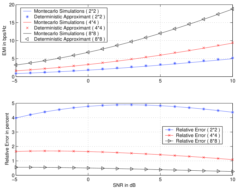
Figure 1: The large system approximation is accurate for correlated Rician MIMO channels. The relative difference between the EMI approximation and that obtained by Monte-Carlo simulations is less than $5\ \%$ for a $2\times 2$ system and less than $1\ \%$ for a $8\times 8$ system.

VI-B Comparison with the Vu-Paulraj method.

In this paragraph, we compare our algorithm with the method presented in [42] based on the maximization of $I({\bf Q})$. We recall that Vu-Paulraj’s algorithm is based on a Newton method and a barrier interior point method. Moreover, the average mutual informations and their first and second derivatives are evaluated by Monte-Carlo simulations. In fig. 3, we have evaluated $C_{E}=\max_{{\bf Q}\in{\cal C}_{1}}I({\bf Q})$ versus the SNR for $r=t=4$. Matrix ${\bf H}$ coincides with the example considered in [42]. The solid line corresponds to the results provided by the Vu-Paulraj’s algorithm; the number of trials used to evaluate the mutual informations and its first and second derivatives is equal to $30.000$, and the maximum number of iterations of the algorithm in [42] is fixed to 10. The dashed line corresponds to the results provided by our algorithm: Each point represents $I(\overline{\bf Q}_{*})$ at the corresponding SNR, where $\overline{\bf Q}_{*}$ is the argmax of $\bar{I}$; the average mutual information at point $\overline{\bf Q}_{*}$ is evaluted by Monte-Carlo simulation (30.000 trials are used). The number of iterations is also limited to 10. Figure 3 shows that our asymptotic approach provides the same results than the Vu-Paulraj’s algorithm. However, our algorithm is computationally much more efficient as the above table shows. The table gives the average executation time (in sec.) of one iteration for both algorithms for $r=t=2,r=t=4,r=t=8$.

In fig. 4, we again compare Vu-Paulraj’s algorithm and our proposal. Matrix ${\bf A}$ is generated according to (4), the angles being chosen at random. The transmit and receive antennas correlations are exponential with parameter $0<\rho_{T}<1$ and $0<\rho_{R}<1$ respectively. In the experiments, $r=t=4$, while various values of $\rho_{T}$, $\rho_{R}$ and of the Rice factor $K$ have been considered. As in the previous experiment, the maximum number of iterations for both algorithms is 10, while the number of trials generated to evaluate the average mutual informations and their derivatives is equal to 30.000. Our approach again provides the same results than Vu-Paulraj’s algorithm, except for low SNRs for $K=1,\rho_{T}=0.5,\rho_{R}=0.8$ where our method gives better results: at these points, the Vu-Paulraj’s algorithm seems not to have converge at the 10th iteration.

	$n=N=2$	$n=N=4$	$n=N=8$
Vu-Paulraj	$0.75$	$8.2$	$138$
New algorithm	$10^{-2}$	$3.10^{-2}$	$7.10^{-2}$

Figure 2: Average time per iteration in seconds

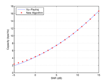
Figure 3: Comparison with the Vu-Paulraj algorithm I

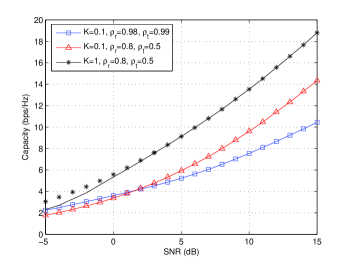
Figure 4: Comparison with the Vu-Paulraj algorithm II

VII Conclusions

In this paper, an explicit approximation for the ergodic mutual information for Rician MIMO channels with transmit and receive antenna correlation is provided. This approximation is based on the asymptotic Random Matrix Theory. The accuracy of the approximation has been studied both analytically and numerically. It has been shown to be very accurate even for small MIMO systems: The relative error is less than $5\%$ for a $2\times 2$ MIMO channel and less $1\ \%$ for an $8\times 8$ MIMO channel.

The derived expression for the EMI has been exploited to derive an efficient optimization algorithm providing the optimum covariance matrix.

Annexe A Proof of the existence and uniqueness of the system (11).

We consider functions $g(\kappa,\tilde{\kappa})$ and $\tilde{g}(\kappa,\tilde{\kappa})$ defined by

$$\begin{array}[]{l}g(\kappa,\tilde{{\kappa}})=\displaystyle{\frac{1}{\kappa}\,\frac{1}{t}\textrm{Tr}\left[{\bf D}\left(\sigma^{2}({\bf I}_{r}+{\bf D}\tilde{\kappa})+{\bf B}({\bf I}_{t}+\tilde{{\bf D}}\kappa)^{-1}{\bf B}^{H}\right)^{-1}\right]}\\ \\ \tilde{g}(\kappa,\tilde{{\kappa}})=\displaystyle{\frac{1}{\tilde{\kappa}}\,\frac{1}{t}\textrm{Tr}\left[\tilde{{\bf D}}\left(\sigma^{2}({\bf I}_{t}+\tilde{{\bf D}}\kappa)+{\bf B}^{H}({\bf I}_{r}+{\bf D}\tilde{\kappa})^{-1}{\bf B}\right)^{-1}\right]}\end{array}.$$ (58)

For each $\tilde{\kappa}>0$ fixed, function $\kappa\rightarrow g(\kappa,\tilde{\kappa})$ is clearly strictly decreasing, converges toward $+\infty$ if $\kappa\rightarrow 0$ and converges to $0$ if $\kappa\rightarrow+\infty$. Therefore, there exists a unique $\kappa>0$ satisfying $g(\kappa,\tilde{\kappa})=1$. As this solution depends on $\tilde{\kappa}$, it is denoted $h(\tilde{\kappa})$ in the following. We claim that

• (i) Function $\tilde{\kappa}\rightarrow h(\tilde{\kappa})$ is strictly decreasing,

• (ii) Function $\tilde{\kappa}\rightarrow\tilde{\kappa}h(\tilde{\kappa})$ is strictly increasing.

In fact, consider $\tilde{\kappa}_{2}>\tilde{\kappa}_{1}$. It is easily checked that for each $\kappa>0$, $g(\kappa,\tilde{\kappa}_{1})>g(\kappa,\tilde{\kappa}_{2})$. Hence, the solution $h(\tilde{\kappa}_{1})$ and $h(\tilde{\kappa}_{2})$ of the equations $g(\kappa,\tilde{\kappa}_{1})=1$ and $g(\kappa,\tilde{\kappa}_{2})=1$ satisfy $h(\tilde{\kappa}_{1})>h(\tilde{\kappa}_{2})$. This establishes (i). To prove (ii), we use the obvious relation $g(h(\tilde{\kappa}_{1}),\tilde{\kappa}_{1})-g(h(\tilde{\kappa}_{2}),\tilde{\kappa}_{2})=0$. We denote by $({\bf U}_{i})_{i=1,2}$ the matrices

$${\bf U}_{i}=\sigma^{2}\left(h(\tilde{\kappa}_{i}){\bf I}+\tilde{\kappa_{i}}h(\tilde{\kappa}_{i}){\bf D}\right)+{\bf B}\left(\frac{{\bf I}}{h(\tilde{\kappa}_{i})}+\tilde{{\bf D}}\right)^{-1}{\bf B}^{H}$$

It is clear that $g(h(\tilde{\kappa}_{i}),\tilde{\kappa}_{i})=\frac{1}{t}\mathrm{Tr}{\bf D}{\bf U}_{i}^{-1}$. We express $g(h(\tilde{\kappa}_{1}),\tilde{\kappa}_{1})-g(h(\tilde{\kappa}_{2}),\tilde{\kappa}_{2})$ as

$$g(h(\tilde{\kappa}_{1}),\tilde{\kappa}_{1})-g(h(\tilde{\kappa}_{2}),\tilde{\kappa}_{2})=\frac{1}{t}\mathrm{Tr}{\bf D}({\bf U}_{1}^{-1}-{\bf U}_{2}^{-1})$$

and use the identity

$${\bf U}_{1}^{-1}-{\bf U}_{2}^{-1}={\bf U}_{1}^{-1}\left({\bf U}_{2}-{\bf U}_{1}\right){\bf U}_{2}^{-1}\ .$$ (59)

Using the form of matrices $({\bf U}_{i})_{i=1,2}$, we eventually obtain that

$$g(h(\tilde{\kappa}_{1}),\tilde{\kappa}_{1})-g(h(\tilde{\kappa}_{2}),\tilde{\kappa}_{2})=u(h(\tilde{\kappa}_{2})-h(\tilde{\kappa}_{1}))+v(\tilde{\kappa}_{2}h(\tilde{\kappa}_{2})-\tilde{\kappa}_{1}h(\tilde{\kappa}_{1}))\ ,$$

where $u$ and $v$ are the strictly positive terms defined by

$$u=\frac{1}{t}\mathrm{Tr}{\bf D}{\bf U}_{1}^{-1}\left(\sigma^{2}{\bf I}+{\bf B}({\bf I}+h(\tilde{\kappa}_{2})\tilde{{\bf D}})^{-1}({\bf I}+h(\tilde{\kappa}_{1})\tilde{{\bf D}})^{-1}{\bf B}^{H}\right){\bf U}_{2}^{-1}$$

and

$$v=\frac{1}{t}\mathrm{Tr}{\bf D}{\bf U}_{1}^{-1}{\bf D}{\bf U}_{2}^{-1}\ .$$

As $u(h(\tilde{\kappa}_{2})-h(\tilde{\kappa}_{1}))+v(\tilde{\kappa}_{2}h(\tilde{\kappa}_{2})-\tilde{\kappa}_{1}h(\tilde{\kappa}_{1}))=0$, $(h(\tilde{\kappa}_{2})-h(\tilde{\kappa}_{1}))<0$ implies that $\tilde{\kappa}_{2}h(\tilde{\kappa}_{2})-\tilde{\kappa}_{1}h(\tilde{\kappa}_{1})>0$. Hence, $\tilde{\kappa}h(\tilde{\kappa})$ is a strictly increasing function as expected.

From this, it follows that function $\tilde{\kappa}\rightarrow\tilde{g}(h(\tilde{\kappa}),\tilde{\kappa})$ is strictly decreasing. This function converges to $+\infty$ if $\tilde{\kappa}\rightarrow 0$ and to $0$ if $\tilde{\kappa}\rightarrow+\infty$. Therefore, the equation

$$\tilde{\kappa}\rightarrow\tilde{g}(h(\tilde{\kappa}),\tilde{\kappa})=1$$

has a unique strictly positive solution $\tilde{\beta}$. If $\beta=h(\tilde{\beta})$, it is clear that $g(\beta,\tilde{\beta})=1$ and $\tilde{g}(\beta,\tilde{\beta})=1$. Therefore, we have shown that $(\beta,\tilde{\beta})$ is the unique solution of (11) satisfying $\beta>0$ and $\tilde{\beta}>0$.

Annexe B Proof of Theorem 2

This section is organized as follows. We first recall in subsection B-A some useful mathematical tools. In subsection B-B, we establish (26). In B-C, we prove (27) and (28).

We shall use the following notations. If $u$ is a random variable, the zero mean random variable $u-\mathbb{E}(u)$ is denoted by $\overset{\circ}{u}$. If $z=x+\mathbf{i}y$ is a complex number, the differential operators $\frac{\partial}{\partial z}$ and $\frac{\partial}{\partial\bar{z}}$ are defined respectively by $\frac{1}{2}\left(\frac{\partial}{\partial x}-\mathbf{i}\frac{\partial}{\partial y}\right)$ and $\frac{1}{2}\left(\frac{\partial}{\partial x}+\mathbf{i}\frac{\partial}{\partial y}\right)$. Finally, if $\boldsymbol{\Sigma},{\bf B},{\bf Y}$ are given matrices, we denote respectively by $\boldsymbol{{\bf\xi}}_{j},{\bf b}_{j},{\bf y}_{j}$ their columns.

B-A Mathematical tools.

B-A1 The Poincaré-Nash inequality

(see e.g. [7], [21]). Let ${\bf x}=[x_{1},\ldots,x_{M}]^{T}$ be a complex Gaussian random vector whose law is given by ${\mathbb{E}}[{\bf x}]={\bf 0}$, ${\mathbb{E}}[{\bf x}{\bf x}^{T}]={\bf 0}$, and ${\mathbb{E}}[{\bf x}{\bf x}^{*}]={\boldsymbol{\Xi}}$. Let $\Phi=\Phi(x_{1},\ldots,x_{M},\bar{x}_{1},\ldots,\bar{x}_{M})$ be a $C^{1}$ complex function polynomially bounded together with its partial derivatives. Then the following inequality holds true:

$$\mathrm{Var}(\Phi({\bf x}))\leq{\mathbb{E}}\left[\nabla_{z}\Phi({\bf x})^{T}\ {\boldsymbol{\Xi}}\ \overline{\nabla_{z}\Phi({\bf x})}\right]+{\mathbb{E}}\left[\left(\nabla_{\bar{z}}\Phi({\bf x})\right)^{H}\ {\boldsymbol{\Xi}}\ \nabla_{\bar{z}}\Phi({\bf x})\right]\ ,$$

where $\nabla_{z}\Phi=[\partial\Phi/\partial z_{1},\ldots,\partial\Phi/\partial z_{M}]^{T}$ and $\nabla_{\bar{z}}\Phi=[\partial\Phi/\partial\bar{z}_{1},\ldots,\partial\Phi/\partial\bar{z}_{M}]^{T}$.

Let ${\bf Y}$ be the $r\times t$ matrix ${\bf Y}=\frac{1}{\sqrt{t}}{\bf D}^{\frac{1}{2}}{\bf X}\tilde{\bf D}^{\frac{1}{2}}$, where ${\bf X}$ has i.i.d. ${\mathcal{C}}N(0,1)$ entries and consider the stacked $rt\times 1$ vector ${\bf x}=[Y_{11},\ldots,Y_{rt}]^{T}$. In this case, Poincaré-Nash inequality writes:

$$\mathrm{Var}\left(\Phi({\bf Y})\right)\leq\frac{1}{t}\sum_{i=1}^{r}\sum_{j=1}^{t}d_{i}\tilde{d}_{j}{\mathbb{E}}\left[\left|\frac{\partial\Phi({\bf Y})}{\partial Y_{i,j}}\right|^{2}+\left|\frac{\partial\Phi({\bf Y})}{\partial\overline{Y}_{i,j}}\right|^{2}\right]\ .$$ (60)

B-A2 The differentiation formula for functions of Gaussian random vectors

With ${\bf x}$ and $\Phi$ given as above, we have the following

$${\mathbb{E}}\left[x_{p}\Phi({\bf x})\right]=\sum_{m=1}^{M}\left[{\boldsymbol{\Xi}}\right]_{pm}{\mathbb{E}}\left[\frac{\partial\Phi({\bf x})}{\partial\bar{x}_{m}}\right]\ .$$ (61)

This formula relies on an integration by parts, and is thus referred to as the Integration by parts formula for Gaussian vectors. It is widely used in Mathematical Physics ([14]) and has been used in Random Matrix Theory in [25] and [32].

If ${\bf x}$ coincides with the $rt\times 1$ vector ${\bf x}=[Y_{11},\ldots,Y_{rt}]^{T}$, relation (61) becomes

$${\mathbb{E}}\left[Y_{pq}\Phi({\bf Y})\right]=\frac{d_{p}\tilde{d}_{q}}{t}{\mathbb{E}}\left[\frac{\partial\Phi({\bf Y})}{\partial\overline{Y}_{pq}}\right]\ .$$ (62)

Replacing matrix ${\bf Y}$ by matrix $\bar{{\bf Y}}$ also provides

$${\mathbb{E}}\left[\overline{Y}_{pq}\Phi({\bf Y})\right]=\frac{d_{p}\tilde{d}_{q}}{t}{\mathbb{E}}\left[\frac{\partial\Phi({\bf Y})}{\partial Y_{pq}}\right]\ .$$ (63)

B-A3 Some useful differentiation formulas

The following partial derivatives $\frac{\partial({\bf S}_{pq})}{\partial Y_{ij}}$ and $\frac{\partial{\bf S}_{pq}}{\partial\overline{Y}_{ij}}$ for each $p,q\in\{1,\ldots,r\}$ and $1\leq i\leq r,1\leq j\leq t$ will be of use in the sequel. Straightforward computations yield:

$$\left\{\begin{array}[]{lcr}\frac{\partial S_{pq}}{\partial Y_{ij}}&=&-S_{p,i}\left({\boldsymbol{\xi}}_{j}^{H}{\bf S}\right)_{q}\\ \frac{\partial S_{pq}}{\partial\bar{Y_{ij}}}&=&-S_{i,q}\left({\bf S}{\boldsymbol{\xi}}\right)_{p}\end{array}\right.\ .$$ (64)

B-B Proof of (26)

We just prove that the variance of $\frac{1}{t}\mbox{Tr}({\bf M}{\bf S})$ is a $O({t^{-2}})$ term. For this, we note that the random variable $\frac{1}{t}\mbox{Tr}({\bf M}{\bf S})$ can be interpreted as a function $\Phi({\bf Y})$ of the entries of matrix ${\bf Y}$, and use the Poincaré-Nash inequality (60) to $\Phi({\bf Y})$. Function $\Phi({\bf Y})$ is equal to

$$\Phi({\bf Y})=\frac{1}{t}\sum_{p,q}M_{q,p}S_{p,q}\ .$$

Therefore, the partial derivative of $\Phi({\bf Y})$ with respect to $Y_{ij}$ is given by $\frac{\partial\Phi({\bf Y})}{\partial Y_{ij}}=\frac{1}{t}\sum_{p,q}{\bf M}_{q,p}\frac{\partial S_{pq}}{\partial Y_{ij}}$ which, by (64), coincides with

$$\frac{\partial\Phi({\bf Y})}{\partial Y_{ij}}=-\frac{1}{t}\sum_{p,q}{\bf M}_{q,p}{\bf S}_{p,i}({\boldsymbol{\xi}}_{j}^{H}{\bf S})_{q}=-\frac{1}{t}\left({\boldsymbol{\xi}}_{j}^{H}{\bf S}{\bf M}{\bf S}\right)_{i}\ .$$

As $d_{i}\leq d_{\max}$ and $\tilde{d}_{j}\leq\tilde{d}_{\max}$, it is clear that

$$\sum_{i=1}^{r}\sum_{j=1}^{t}d_{i}\tilde{d}_{j}\mathbb{E}\left|\frac{\partial\Phi({\bf Y})}{\partial Y_{ij}}\right|^{2}\leq d_{\max}\tilde{d}_{\max}\sum_{i=1}^{r}\sum_{j=1}^{t}\mathbb{E}\left|\frac{\partial\Phi({\bf Y})}{\partial Y_{ij}}\right|^{2}\ .$$

It is easily seen that

$$\sum_{i=1}^{r}\mathbb{E}\left|\frac{\partial\Phi({\bf Y})}{\partial Y_{ij}}\right|^{2}=\frac{1}{t^{2}}\mathbb{E}\left({\boldsymbol{\xi}}_{j}^{H}{\bf S}{\bf M}{\bf S}^{2}{\bf M}^{H}{\bf S}{\boldsymbol{\xi}}_{j}^{H}\right)\ .$$

As $\|{\bf S}\|\leq\frac{1}{\sigma^{2}}$ and $\sup_{t}\|{\bf M}\|<\infty$, ${\boldsymbol{\xi}}_{j}^{H}{\bf S}{\bf M}{\bf S}^{2}{\bf M}^{H}{\bf S}{\boldsymbol{\xi}}_{j}^{H}$ is less than $\frac{1}{\sigma^{8}}\sup_{t}\|{\bf M}\|^{2}\;\|{\boldsymbol{\xi}}_{j}\|^{2}$. Moreover, $\mathbb{E}\|{\boldsymbol{\xi}}_{j}\|^{2}$ coincides with $\|{\bf b}_{j}\|^{2}+\frac{1}{t}\tilde{d}_{j}\sum_{i=1}^{r}d_{i}$, which is itself less than $b_{\max}^{2}+d_{\max}\tilde{d}_{\max}\frac{r}{t}$, a uniformly bounded term. Therefore, $\sum_{i=1}^{r}\mathbb{E}\left|\frac{\partial\Phi({\bf Y})}{\partial Y_{ij}}\right|^{2}$ is a $O({t^{-2}})$ term. This proves that

$$\frac{1}{t}\sum_{i=1}^{r}\sum_{j=1}^{t}d_{i}\tilde{d}_{j}\mathbb{E}\left|\frac{\partial\Phi({\bf Y})}{\partial Y_{ij}}\right|^{2}=O\left(\frac{1}{t^{2}}\right)\ .$$

It can be shown similarly that ${t}^{-1}\sum_{i=1}^{r}\sum_{j=1}^{t}d_{i}\tilde{d}_{j}\mathbb{E}\left|\frac{\partial\Phi({\bf Y})}{\partial\overline{Y_{ij}}}\right|^{2}=O\left({t^{-2}}\right)\ .$ The conclusion follows from Poincaré-Nash inequality (60).

B-C Proof of (27) and (28).

As we shall see, proofs of (27) and (28) are demanding. We first introduce the following notations: Define scalar parameters $\eta(\sigma^{2}),\alpha(\sigma^{2}),\tilde{\alpha}(\sigma^{2})$ as

$$\begin{array}[]{ccc}\eta(\sigma^{2})&=&\frac{1}{t}\mbox{Tr}\left({\bf D}{\bf S}(\sigma^{2})\right)\\ \alpha(\sigma^{2})&=&{\mathbb{E}}\left[\frac{1}{t}\mbox{Tr}\left({\bf D}{\bf S}(\sigma^{2})\right)\right]\\ \tilde{\alpha}(\sigma^{2})&=&{\mathbb{E}}\left[\frac{1}{t}\mbox{Tr}\left(\tilde{{\bf D}}\tilde{{\bf S}}(\sigma^{2})\right)\right]\end{array}$$ (65)

and matrices ${\bf R}(\sigma^{2}),\tilde{{\bf R}}(\sigma^{2})$ as

$$\begin{array}[]{ccc}{\bf R}(\sigma^{2})&=&\left[\sigma^{2}\left({\bf I}+\tilde{\alpha}{\bf D}\right)+{\bf B}\left({\bf I}+\alpha\tilde{{\bf D}}\right)^{-1}{\bf B}^{H}\right]^{-1}\\ \tilde{{\bf R}}(\sigma^{2})&=&\left[\sigma^{2}\left({\bf I}+\alpha\tilde{\bf D}\right)+{\bf B}^{H}\left({\bf I}+\tilde{\alpha}{{\bf D}}\right)^{-1}{\bf B}\right]^{-1}\end{array}\ .$$ (66)

We note that, as $\alpha(\sigma^{2})\geq 0$ and $\tilde{\alpha}(\sigma^{2})\geq 0$, then

$$0<{\bf R}(\sigma^{2})<\frac{{\bf I}_{r}}{\sigma^{2}},\;0<\tilde{{\bf R}}(\sigma^{2})<\frac{{\bf I}_{t}}{\sigma^{2}}$$ (67)

It is difficult to study directly the term $\frac{1}{r}\mathrm{Tr}{\bf M}(\mathbb{E}({\bf S})-{\bf T})$. In some sense, matrix ${\bf R}$ can be seen as an intermediate quantity between $\mathbb{E}({\bf S})$ and ${\bf T}$. Thus the proof consists into two steps: 1) for each uniformly bounded matrix ${\bf M}$, we first prove that $\frac{1}{r}\mathrm{Tr}{\bf M}(\mathbb{E}({\bf S})-{\bf R})$ and $\frac{1}{r}\mathrm{Tr}{\bf M}({\bf R}-{\bf T})$ converge to $0$ as $t\to\infty$; 2) we then refine the previous result and establish in fact that $\frac{1}{r}\mathrm{Tr}{\bf M}(\mathbb{E}({\bf S})-{\bf R})$ and $\frac{1}{r}\mathrm{Tr}{\bf M}({\bf R}-{\bf T})$ are $O({t^{-2}})$ terms. This, of course, imply (27). Eq. (28) eventually follows from Eq. (27), the integral representation

$$\overline{J}(\sigma^{2})-J(\sigma^{2})=\int_{\sigma^{2}}^{\infty}\mathrm{Tr}\left(\mathrm{E}({\bf S}(\omega))-{\bf T}(\omega)\right)\,d\,\omega,$$ (68)

which follows from (20) and (22), as well as a dominated convergence argument that is omitted.

B-C1 First step: Convergence of $\frac{1}{r}\mathrm{Tr}{\bf M}(\mathbb{E}({\bf S})-{\bf R})$ and $\frac{1}{r}\mathrm{Tr}{\bf M}({\bf R}-{\bf T})$ to zero

The first step consists in showing the following Proposition.

Proposition 7

For each deterministic $r\times r$ matrix ${\bf M}$, uniformly bounded (for the spectral norm) as $t\to\infty$, we have:

$$\lim_{t\to+\infty}\frac{1}{t}\mathrm{Tr}\left[{\bf M}\left(\mathbb{E}({\bf S})-{\bf R}\right)\right]=0$$ (69)

$$\lim_{t\to+\infty}\frac{1}{t}\mathrm{Tr}\left[{\bf M}\left({\bf R})-{\bf T}\right)\right]=0$$ (70)

Proof:

We first prove (69). For this, we state the following useful Lemma.

Lemma 2

Let ${\bf P},{\bf P}_{1}$ and ${\bf P}_{2}$ be deterministic $r\times t,t\times t,t\times r$ matrices respectively, uniformly bounded with respect to the spectral norm as $t\to\infty$. Consider the following functions of ${\bf Y}$.

$$\boldsymbol{\Phi}({\bf Y})=\frac{1}{t}\mbox{Tr}\left[{\bf S}{\bf P}{\boldsymbol{\Sigma}}^{H}\right],\quad\boldsymbol{\Psi}({\bf Y})=\frac{1}{t}\mbox{Tr}\left[{\bf S}{\boldsymbol{\Sigma}}{\bf P}_{1}{\boldsymbol{\Sigma}}^{H}{\bf P}_{2}\right],\quad\boldsymbol{\Psi}^{{}^{\prime}}({\bf Y})=\frac{1}{t}\mbox{Tr}\left[{\bf S}{\boldsymbol{\Sigma}}{\bf P}_{1}{\bf{Y}}^{H}{\bf P}_{2}\right]\ .$$

Then, the following estimates hold true:

$$\mbox{Var}(\boldsymbol{\Phi})=O\left(\frac{1}{t^{2}}\right),\quad\mbox{Var}(\boldsymbol{\Psi})=O\left(\frac{1}{t^{2}}\right),\quad\mbox{Var}(\boldsymbol{\Psi}^{{}^{\prime}})=O\left(\frac{1}{t^{2}}\right)\ .$$

The proof, based on the Poincaré-Nash inequality (60), is omitted.

In order to use the Integration by parts formula (62), notice that

$$\sigma^{2}{\bf S}(\sigma^{2})+{\bf S}(\sigma^{2}){\boldsymbol{\Sigma}}{\boldsymbol{\Sigma}}^{H}={\bf I}\ .$$ (71)

Taking the mathematical expectation, we have for each $p,q\in\{1,\ldots,r\}$:

$$\sigma^{2}\mathbb{E}(S_{pq})+\mathbb{E}\left[({\bf S}{\boldsymbol{\Sigma}}{\boldsymbol{\Sigma}}^{H})_{pq}\right]=\delta(p-q)\ .$$ (72)

A convenient use of the Integration by parts formula allows to express $\mathbb{E}\left[({\bf S}{\boldsymbol{\Sigma}}{\boldsymbol{\Sigma}}^{H})_{pq}\right]$ in terms of the entries of $\mathbb{E}({\bf S})$. To see this, note that

$$\mathbb{E}\left[({\bf S}{\boldsymbol{\Sigma}}{\boldsymbol{\Sigma}}^{H})_{pq}\right]=\sum_{j=1}^{t}\sum_{i=1}^{r}\mathbb{E}(S_{pi}\Sigma_{ij}\overline{\Sigma_{qj}})\ .$$

For each $i$, $\mathbb{E}(S_{pi}\Sigma_{ij}\overline{\Sigma_{qj}})$ can be written as

$$\mathbb{E}(S_{pi}\Sigma_{ij}\overline{\Sigma_{qj}})=\mathbb{E}(S_{pi})B_{ij}\overline{B_{qj}}+\mathbb{E}\left(S_{pi}\overline{Y_{qj}}\right)B_{ij}+\mathbb{E}\left(S_{pi}Y_{ij}\overline{\Sigma_{qj}}\right)\ .$$

Using (62) with function $\Phi({\bf Y})=S_{pi}\overline{\Sigma_{qj}}$ and (63) with $\Phi({\bf Y})=S_{pi}$, and summing over index $i$ yields:

$$\mathbb{E}\left[({\bf S}{\boldsymbol{\xi}}_{j})_{p}\overline{\Sigma_{q,j}}\right]=\frac{d_{q}\tilde{d}_{j}}{t}\mathbb{E}(S_{pq})-\tilde{d}_{j}{\mathbb{E}}\left[\eta({\bf S}{\boldsymbol{\xi}}_{j})_{p}\overline{\Sigma_{q,j}}\right]-\frac{d_{q}\tilde{d}_{j}}{t}{\mathbb{E}}\left[S_{pq}{\boldsymbol{\xi}}_{j}^{H}{\bf S}{\bf b}_{j}\right]+{\mathbb{E}}\left[({\bf S}{\bf b}_{j})_{p}\right]\overline{B_{qj}}\ .$$ (73)

Eq. (26) for ${\bf M}={\bf D}$ implies that $\mathrm{Var}(\eta)=O({t^{-2}})$, or equivalently that $\mathbb{E}(\overset{\circ}{\eta}^{2})=O({t^{-2}})$. We now complete proof of (69). We take Eq. (73) as a starting point, and write $\eta$ as $\eta=\mathbb{E}(\eta)+\overset{\circ}{\eta}=\alpha+\overset{\circ}{\eta}$. Therefore,

$$\mathbb{E}\left[\eta\,({\bf S}\boldsymbol{\xi}_{j})_{p}\,\overline{{\Sigma}_{q,j}}\right]=\alpha\mathbb{E}\left[({\bf S}\boldsymbol{\xi}_{j})_{p}\,\overline{{\Sigma}_{q,j}}\right]+\mathbb{E}\left[\overset{\circ}{\eta}\,({\bf S}\boldsymbol{\xi}_{j})_{p}\,\overline{{\Sigma}_{q,j}}\right]\ .$$

Plugging this relation into (73), and solving w.r.t. $\mathbb{E}\left[({\bf S}\boldsymbol{\xi}_{j})_{p}\,\overline{{\Sigma}_{q},j}\right]$ yields

$$\mathbb{E}\left[({\bf S}{\boldsymbol{\xi}}_{j})_{p}\overline{\Sigma_{q,j}}\right] = \frac{1}{t}\frac{d_{q}\tilde{d}_{j}}{1+\alpha\tilde{d}_{j}}{\mathbb{E}}(S_{pq})+\frac{1}{1+\alpha\tilde{d}_{j}}{\mathbb{E}}\left[({\bf S}{\bf b}_{j})_{p}\right]\overline{B_{qj}}$$

$$-\,\frac{1}{t}\frac{d_{q}\tilde{d}_{j}}{1+\alpha\tilde{d}_{j}}{\mathbb{E}}\left[S_{pq}{\boldsymbol{\xi}}_{j}^{H}{\bf S}{\bf b}_{j}\right]-\frac{\tilde{d}_{j}}{1+\alpha\tilde{d}_{j}}\mathbb{E}\left[\overset{\circ}{\eta}\,({\bf S}\boldsymbol{\xi}_{j})_{p}\,\overline{{\Sigma}_{q,j}}\right]\ .$$

Writing ${\boldsymbol{\xi}}_{j}={\bf b}_{j}+{\bf y}_{j}$, and summing over $j$ provides the following expression of $\mathbb{E}\left[({\bf S}{\boldsymbol{\Sigma}}{\boldsymbol{\Sigma}}^{H})_{pq}\right]$:

$$\mathbb{E}\left[({\bf S}{\boldsymbol{\Sigma}}{\boldsymbol{\Sigma}}^{H})_{pq}\right]\quad=\quad d_{q}\,\frac{1}{t}\mathrm{Tr}\left[\tilde{{\bf D}}({\bf I}+\alpha\tilde{{\bf D}})^{-1}\right]\mathbb{E}(S_{pq})\\ +{\mathbb{E}}\left[\left({\bf S}{\bf B}({\bf I}+\alpha\tilde{{\bf D}})^{-1}{\bf B}^{H}\right)_{pq}\right]-d_{q}\,{\mathbb{E}}\left[S_{pq}\frac{1}{t}\mathrm{Tr}\left({\bf S}{\bf B}\tilde{{\bf D}}({\bf I}+\alpha\tilde{{\bf D}})^{-1}{\bf B}^{H}\right)\right]\\ -d_{q}\,{\mathbb{E}}\left[S_{pq}\frac{1}{t}\mathrm{Tr}\left({\bf S}{\bf B}\tilde{{\bf D}}({\bf I}+\alpha\tilde{{\bf D}})^{-1}{\bf Y}^{H}\right)\right]-\mathbb{E}\left[\overset{\circ}{\eta}\left({\bf S}{\boldsymbol{\Sigma}}\tilde{{\bf D}}({\bf I}+\alpha\tilde{{\bf D}})^{-1}{\boldsymbol{\Sigma}}^{H}\right)_{p,q}\right]\ .$$ (74)

The resolvent identity (71) thus implies that

$$\delta(p-q)\quad=\quad\sigma^{2}{\mathbb{E}}(S_{pq})+\frac{d_{q}}{t}\mathrm{Tr}\left[\tilde{{\bf D}}({\bf I}+\alpha\tilde{{\bf D}})^{-1}\right]\mathbb{E}(S_{pq})\\ +{\mathbb{E}}\left[\left({\bf S}{\bf B}({\bf I}+\alpha\tilde{{\bf D}})^{-1}{\bf B}^{H}\right)_{pq}\right]-d_{q}\,{\mathbb{E}}\left[S_{pq}\frac{1}{t}\mathrm{Tr}\left({\bf S}{\bf B}\tilde{{\bf D}}({\bf I}+\alpha\tilde{{\bf D}})^{-1}{\bf B}^{H}\right)\right]\\ -d_{q}\,{\mathbb{E}}\left[S_{pq}\frac{1}{t}\mathrm{Tr}\left({\bf S}{\bf B}\tilde{{\bf D}}({\bf I}+\alpha\tilde{{\bf D}})^{-1}{\bf Y}^{H}\right)\right]-\mathbb{E}\left[\overset{\circ}{\eta}\left({\bf S}{\boldsymbol{\Sigma}}\tilde{{\bf D}}({\bf I}+\alpha\tilde{{\bf D}})^{-1}{\boldsymbol{\Sigma}}^{H}\right)_{p,q}\right]\ .$$ (75)

In order to simplify the notations, we define $\rho_{1}$ and $\rho_{2}$ by

$$\rho_{1}\ =\ \frac{1}{t}\mathrm{Tr}\left({\bf S}{\bf B}\tilde{{\bf D}}({\bf I}+\alpha\tilde{{\bf D}})^{-1}{\bf B}^{H}\right)\quad\textrm{and}\quad\rho_{2}\ =\ \frac{1}{t}\mathrm{Tr}\left({\bf S}{\bf B}\tilde{{\bf D}}({\bf I}+\alpha\tilde{{\bf D}})^{-1}{\bf Y}^{H}\right)\ .$$

For $i=1,2$, we write ${\mathbb{E}}(S_{pq}\rho_{i})$ as

$${\mathbb{E}}(S_{pq}\rho_{i})={\mathbb{E}}(S_{pq})\,{\mathbb{E}}(\rho_{i})+{\mathbb{E}}\left(\overset{\circ}{S_{pq}}\;\overset{\circ}{\rho_{i}}\right)\ .$$

Thus, (75) can be written as

$$\delta(p-q)\quad=\quad\sigma^{2}{\mathbb{E}}(S_{pq})+d_{q}\,\frac{1}{t}\mathrm{Tr}\left[\tilde{{\bf D}}({\bf I}+\alpha\tilde{{\bf D}})^{-1}\right]\mathbb{E}(S_{pq})\\ +\left({\mathbb{E}}({\bf S}){\bf B}({\bf I}+\alpha\tilde{{\bf D}})^{-1}{\bf B}^{H}\right)_{pq}-d_{q}\,{\mathbb{E}}(S_{pq})\frac{1}{t}\mathrm{Tr}\left({\mathbb{E}}({\bf S}){\bf B}\tilde{{\bf D}}({\bf I}+\alpha\tilde{{\bf D}})^{-1}{\bf B}^{H}\right)\\ -d_{q}\,{\mathbb{E}}(S_{pq}){\mathbb{E}}\left[\frac{1}{t}\mathrm{Tr}\left({\bf S}{\bf B}\tilde{{\bf D}}({\bf I}+\alpha\tilde{{\bf D}})^{-1}{\bf Y}^{H}\right)\right]-d_{q}\,{\mathbb{E}}\left(\overset{\circ}{S_{pq}}\;\overset{\circ}{\rho_{1}}\right)-d_{q}\,{\mathbb{E}}\left(\overset{\circ}{S_{pq}}\;\overset{\circ}{\rho_{2}}\right)\\ -\mathbb{E}\left[\overset{\circ}{\eta}\left({\bf S}{\boldsymbol{\Sigma}}\tilde{{\bf D}}({\bf I}+\alpha\tilde{{\bf D}})^{-1}{\boldsymbol{\Sigma}}^{H}\right)_{p,q}\right]\ .$$ (76)

We now establish the following lemma.

Lemma 3

$${\mathbb{E}}\rho_{2} = {\mathbb{E}}\left[\frac{1}{t}\mathrm{Tr}\left({\bf S}{\bf B}\tilde{{\bf D}}({\bf I}+\alpha\tilde{{\bf D}})^{-1}{\bf Y}^{H}\right)\right]$$ (77)

$$= -\alpha\,\frac{1}{t}\mathrm{Tr}\left(\mathbb{E}({\bf S}){\bf B}\tilde{{\bf D}}^{2}({\bf I}+\alpha\tilde{{\bf D}})^{-2}{\bf B}^{H}\right)-{\mathbb{E}}\left(\overset{\circ}{\eta}\;\overset{\circ}{\rho_{3}}\right)\ ,$$

where $\rho_{3}$ is defined by

$$\rho_{3}=\frac{1}{t}\mathrm{Tr}\left({\bf S}{\bf B}\tilde{{\bf D}}^{2}({\bf I}+\alpha\tilde{{\bf D}})^{-2}{\boldsymbol{\Sigma}}^{H}\right)\ .$$

Proof:

We express ${\mathbb{E}}(\rho_{2})$ as

$$\begin{array}[]{ccc}{\mathbb{E}}(\rho_{2})&=&\frac{1}{t}\sum_{j=1}^{t}\frac{\tilde{d}_{j}}{1+\alpha\tilde{d}_{j}}\;{\mathbb{E}}({\bf y}_{j}^{H}{\bf S}{\bf b}_{j})\\ &=&\frac{1}{t}\sum_{j=1}^{t}\frac{\tilde{d}_{j}}{1+\alpha\tilde{d}_{j}}\,\sum_{i=1}^{r}{\mathbb{E}}\left(({\bf S}{\bf b}_{j})_{i}\overline{Y_{ij}}\right)\end{array}$$ (78)

and evaluate ${\mathbb{E}}\left(({\bf S}{\bf b}_{j})_{i}\overline{Y_{ij}}\right)$ using formula (63) for $\Phi({\bf Y})=({\bf S}{\bf b}_{j})_{i}$. This gives

$${\mathbb{E}}\left(({\bf S}{\bf b}_{j})_{i}\overline{Y_{ij}}\right)=\frac{1}{t}d_{i}\tilde{d}_{j}\sum_{k=1}^{r}{\mathbb{E}}\left(\frac{\partial S_{ik}}{\partial Y_{ij}}\right)B_{kj}\ .$$

By (64),

$${\mathbb{E}}\left(\frac{\partial S_{ik}}{\partial Y_{ij}}\right)=-{\mathbb{E}}\left(S_{ii}({\bf b}_{j}^{H}{\bf S})_{k}\right)-{\mathbb{E}}\left(S_{ii}({\bf y}_{j}^{H}{\bf S})_{k}\right)\ .$$

Therefore,

$${\mathbb{E}}\left({\bf y}_{j}^{H}{\bf S}{\bf b}_{j}\right)=-\tilde{d}_{j}{\mathbb{E}}\left(\eta\,{\bf b}_{j}^{H}{\bf S}{\bf b}_{j}\right)-\tilde{d}_{j}{\mathbb{E}}\left(\eta\,{\bf y}_{j}^{H}{\bf S}{\bf b}_{j}\right)\ .$$

Writing again $\eta={\mathbb{E}}(\eta)+\overset{\circ}{\eta}=\alpha+\overset{\circ}{\eta}$, we get that

$$\begin{array}[]{ccc}{\mathbb{E}}\left({\bf y}_{j}^{H}{\bf S}{\bf b}_{j}\right)&=&-\alpha\tilde{d}_{j}{\mathbb{E}}\left({\bf b}_{j}^{H}{\bf S}{\bf b}_{j}\right)-\alpha\tilde{d}_{j}{\mathbb{E}}\left({\bf y}_{j}^{H}{\bf S}{\bf b}_{j}\right)\\ &&-\tilde{d}_{j}{\mathbb{E}}\left(\overset{\circ}{\eta}\,{\bf b}_{j}^{H}{\bf S}{\bf b}_{j}\right)-\tilde{d}_{j}{\mathbb{E}}\left(\overset{\circ}{\eta}\,{\bf y}_{j}^{H}{\bf S}{\bf b}_{j}\right)\ .\end{array}$$ (79)

Solving this equation w.r.t. ${\mathbb{E}}\left({\bf y}_{j}^{H}{\bf S}{\bf b}_{j}\right)$ yields

$${\mathbb{E}}\left({\bf y}_{j}^{H}{\bf S}{\bf b}_{j}\right)=-\frac{\alpha\tilde{d}_{j}}{1+\alpha\tilde{d}_{j}}{\mathbb{E}}\left({\bf b}_{j}^{H}{\bf S}{\bf b}_{j}\right)-\frac{\tilde{d}_{j}}{1+\alpha\tilde{d}_{j}}{\mathbb{E}}\left(\overset{\circ}{\eta}\,{\bf b}_{j}^{H}{\bf S}{\bf b}_{j}\right)-\frac{\tilde{d}_{j}}{1+\alpha\tilde{d}_{j}}{\mathbb{E}}\left(\overset{\circ}{\eta}\,{\bf y}_{j}^{H}{\bf S}{\bf b}_{j}\right)$$ (80)

or equivalently

$${\mathbb{E}}\left({\bf y}_{j}^{H}{\bf S}{\bf b}_{j}\right)=-\frac{\alpha\tilde{d}_{j}}{1+\alpha\tilde{d}_{j}}{\mathbb{E}}\left({\bf b}_{j}^{H}{\bf S}{\bf b}_{j}\right)-\frac{\tilde{d}_{j}}{1+\alpha\tilde{d}_{j}}{\mathbb{E}}\left(\overset{\circ}{\eta}\,{\boldsymbol{\xi}}_{j}^{H}{\bf S}{\bf b}_{j}\right)\ .$$ (81)

Eq. (77) immediately follows from (78), (81), and the relation $\mathbb{E}(\overset{\circ}{\eta}\,\rho_{3})=\mathbb{E}(\overset{\circ}{\eta}\,\overset{\circ}{\rho_{3}})$. ∎

Plugging (77) into (76) yields

$$\delta(p-q)+\Delta_{pq}\\ ={\mathbb{E}}(S_{pq})\left[\sigma^{2}+d_{q}\left(\frac{1}{t}\mathrm{Tr}\tilde{{\bf D}}({\bf I}+\alpha\tilde{{\bf D}})^{-1}-{\mathbb{E}}(\rho_{1})+\alpha\frac{1}{t}\mathrm{Tr}{\mathbb{E}}({\bf S}){\bf B}\tilde{{\bf D}}^{2}({\bf I}+\alpha\tilde{{\bf D}})^{-2}{\bf B}^{H}\right)\right]\\ +\left[{\mathbb{E}}({\bf S}){\bf B}({\bf I}+\alpha\tilde{{\bf D}})^{-1}{\bf B}^{H}\right]_{pq}$$ (82)

where ${\boldsymbol{\Delta}}$ is the $r\times r$ matrix defined by

$$\Delta_{pq}={\mathbb{E}}\left[\overset{\circ}{\eta}\left({\bf S}{\boldsymbol{\Sigma}}\tilde{{\bf D}}({\bf I}+\alpha\tilde{{\bf D}})^{-1}{\boldsymbol{\Sigma}}^{H}\right)_{pq}\right]+d_{q}{\mathbb{E}}\left(\overset{\circ}{S}_{pq}(\overset{\circ}{\rho_{1}}+\overset{\circ}{\rho_{2}})\right)-d_{q}{\mathbb{E}}(S_{pq})\,{\mathbb{E}}\left(\overset{\circ}{\eta}\,\overset{\circ}{\rho_{3}}\right)$$

for each $p,q$ or equivalently by

$${\boldsymbol{\Delta}}={\mathbb{E}}\left[\overset{\circ}{\eta}\left({\bf S}{\boldsymbol{\Sigma}}\tilde{{\bf D}}({\bf I}+\alpha\tilde{{\bf D}})^{-1}{\boldsymbol{\Sigma}}^{H}\right)\right]+{\mathbb{E}}\left((\overset{\circ}{\rho_{1}}+\overset{\circ}{\rho_{2}})\,\overset{\circ}{{\bf S}}\right)\,{\bf D}-{\mathbb{E}}\left(\overset{\circ}{\eta}\,\overset{\circ}{\rho_{3}}\right)\,{\mathbb{E}}({\bf S})\,{\bf D}\ .$$

Using the relation $\alpha\tilde{{\bf D}}({\bf I}+\alpha\tilde{{\bf D}})^{-1}={\bf I}-({\bf I}+\alpha\tilde{{\bf D}})^{-1}$, we obtain that

$$\alpha\frac{1}{t}\mathrm{Tr}\left({\mathbb{E}}({\bf S}){\bf B}\tilde{{\bf D}}^{2}({\bf I}+\alpha\tilde{{\bf D}})^{-2}{\bf B}^{H}\right)$$ (83)

$$= \frac{1}{t}\mathrm{Tr}\left({\mathbb{E}}({\bf S}){\bf B}\tilde{{\bf D}}({\bf I}+\alpha\tilde{{\bf D}})^{-1}{\bf B}^{H}\right)-\frac{1}{t}\mathrm{Tr}\left({\mathbb{E}}({\bf S}){\bf B}\tilde{{\bf D}}({\bf I}+\alpha\tilde{{\bf D}})^{-2}{\bf B}^{H}\right)$$

$$= {\mathbb{E}}(\rho_{1})-\frac{1}{t}\mathrm{Tr}\left({\mathbb{E}}({\bf S}){\bf B}\tilde{{\bf D}}({\bf I}+\alpha\tilde{{\bf D}})^{-2}{\bf B}^{H}\right)\ .$$

Therefore, the term

$$\frac{1}{t}\mathrm{Tr}\tilde{{\bf D}}({\bf I}+\alpha\tilde{{\bf D}})^{-1}-{\mathbb{E}}(\rho_{1})+\alpha\frac{1}{t}\mathrm{Tr}\left({\mathbb{E}}({\bf S}){\bf B}\tilde{{\bf D}}^{2}({\bf I}+\alpha\tilde{{\bf D}})^{-2}{\bf B}^{H}\right)$$

is equal to

$$\frac{1}{t}\mathrm{Tr}\tilde{{\bf D}}({\bf I}+\alpha\tilde{{\bf D}})^{-1}-\frac{1}{t}\mathrm{Tr}\left({\mathbb{E}}({\bf S}){\bf B}\tilde{{\bf D}}({\bf I}+\alpha\tilde{{\bf D}})^{-2}{\bf B}^{H}\right)\\ =\frac{1}{t}\mathrm{Tr}\left[\tilde{{\bf D}}({\bf I}+\alpha\tilde{{\bf D}})^{-1}\left({\bf I}-{\bf B}^{H}{\mathbb{E}}({\bf S}){\bf B}({\bf I}+\alpha\tilde{{\bf D}})^{-1}\right)\right]$$

which, in turn, coincides with $\sigma^{2}\,\tilde{\tau}$, where $\tilde{\tau}$ is defined by

$$\tilde{\tau}(\sigma^{2})=\frac{1}{t}\mbox{Tr}\left[\tilde{{\bf D}}\left(\sigma^{2}({\bf I}+\alpha\tilde{{\bf D}})\right)^{-1}\left({\bf I}-{\bf B}^{H}\,\mathbb{E}({\bf S}(\sigma^{2}))\,{\bf B}({\bf I}+\alpha\tilde{{\bf D}})^{-1}\right)\right]$$ (84)

Eq. (82) is thus equivalent to

$$\left({\mathbb{E}}({\bf S})\left[\sigma^{2}({\bf I}+\tilde{\tau}{\bf D})+{\bf B}({\bf I}+\alpha\tilde{{\bf D}})^{-1}{\bf B}^{H}\right]\right)={\bf I}+{\boldsymbol{\Delta}}$$ (85)

or equivalently to

$$\left({\mathbb{E}}\left[{\bf S}\left(\sigma^{2}({\bf I}+\tilde{\alpha}{\bf D})+{\bf B}({\bf I}+\alpha\tilde{{\bf D}})^{-1}{\bf B}^{H}\right)\right]\right)={\bf I}+\sigma^{2}(\tilde{\alpha}-\tilde{\tau})\mathbb{E}({\bf S}){\bf D}+\boldsymbol{\Delta}$$

or to

$${\mathbb{E}}({\bf S})={\bf R}+\sigma^{2}(\tilde{\alpha}-\tilde{\tau})\mathbb{E}({\bf S}){\bf D}{\bf R}+\boldsymbol{\Delta}{\bf R}\ .$$ (86)

We now verify that if ${\bf M}$ is a deterministic, uniformly bounded matrix for the spectral norm as $t\to\infty$, then ${t}^{-1}\mathrm{Tr}{\boldsymbol{\Delta}}{\bf R}{\bf M}=O\left({t^{-2}}\right)\ .$ For this, we write $\frac{1}{t}\,\mathrm{Tr}{\boldsymbol{\Delta}}{\bf R}{\bf M}$ as $\frac{1}{t}\,\mathrm{Tr}{\boldsymbol{\Delta}}{\bf R}{\bf M}=T_{1}+T_{2}-T_{3}$ where

$$\begin{array}[]{ccc}T_{1}&=&{\mathbb{E}}\left[\overset{\circ}{\eta}\;\frac{1}{t}\mathrm{Tr}\left({\bf S}{\boldsymbol{\Sigma}}\tilde{{\bf D}}({\bf I}+\alpha\tilde{{\bf D}})^{-1}{\boldsymbol{\Sigma}}^{H}{\bf R}{\bf M}\right)\right]\ ,\\ T_{2}&=&{\mathbb{E}}\left((\overset{\circ}{\rho_{1}}+\overset{\circ}{\rho_{2}})\,\frac{1}{t}\,\mathrm{Tr}(\overset{\circ}{{\bf S}}{\bf D}{\bf R}{\bf M})\right)\ ,\\ T_{3}&=&{\mathbb{E}}\left(\overset{\circ}{\eta}\,\overset{\circ}{\rho_{3}}\right)\,\frac{1}{t}\,\mathrm{Tr}\left({\mathbb{E}}({\bf S}){\bf D}{\bf R}{\bf M}\right)\ .\end{array}$$

We denote by $\rho_{4}$ the term

$$\rho_{4}=\frac{1}{t}\mathrm{Tr}\left({\bf S}{\boldsymbol{\Sigma}}\tilde{{\bf D}}({\bf I}+\alpha\tilde{{\bf D}})^{-1}{\boldsymbol{\Sigma}}^{H}{\bf R}{\bf M}\right)$$

and notice that $T_{1}={\mathbb{E}}(\overset{\circ}{\eta}\;\overset{\circ}{\rho_{4}})$. Eq. (26) implies that ${\mathbb{E}}(\overset{\circ}{\eta}^{2})$ and ${\mathbb{E}}\left[\frac{1}{t}\,\mathrm{Tr}\left(\overset{\circ}{{\bf S}}{\bf D}{\bf R}{\bf M})\right)\right]^{2}$ are $O({t^{-2}})$ terms. Moreover, matrix ${\bf R}$ is uniformly bounded for the spectral norm as $t\to\infty$ (see (67). Lemma 2 immediately shows that for each $i=1,2,3$, ${\mathbb{E}}(\overset{\circ}{\rho_{i}}^{2})$ is a $O({t^{-2}})$ term. The Cauchy-Schwarz inequality eventually provides $\frac{1}{t}\mathrm{Tr}{\boldsymbol{\Delta}}{\bf R}{\bf M}=O({t^{-2}})$.

In order to establish (69), it remains to show that $\tilde{\alpha}-\tilde{\tau}\to 0$. For this, we remark that exchanging the roles of matrices $\boldsymbol{\Sigma}$ and $\boldsymbol{\Sigma}^{H}$ leads to the following relation

$${\mathbb{E}}(\tilde{{\bf S}})=\tilde{{\bf R}}+\sigma^{2}(\alpha-\tau)\mathbb{E}(\tilde{{\bf S}}\tilde{{\bf D}}\tilde{{\bf R}})+\tilde{\boldsymbol{\Delta}}\tilde{{\bf R}}$$ (87)

where $\tau(\sigma^{2})$ is defined by

$$\tau(\sigma^{2})=\frac{1}{t}\mbox{Tr}\left[{\bf D}\left(\sigma^{2}({\bf I}+\tilde{\alpha}{\bf D})\right)^{-1}\left({\bf I}-{\bf B}\,\mathbb{E}(\tilde{{\bf S}}(\sigma^{2}))\,{\bf B}^{H}({\bf I}+\tilde{\alpha}{\bf D})^{-1}\right)\right]$$ (88)

and where $\tilde{\boldsymbol{\Delta}}$, the analogue of $\boldsymbol{\Delta}$, satisfies

$$\frac{1}{t}\mathrm{Tr}(\tilde{\boldsymbol{\Delta}}\tilde{{\bf M}})=O\left(\frac{1}{t^{2}}\right)$$ (89)

for every matrix $\tilde{{\bf M}}$ uniformly bounded for the spectral norm.

Equations (86) and (87) allow to evaluate $\tilde{\alpha}$ and $\tilde{\tau}$. More precisely, writing $\tilde{\alpha}=\frac{1}{t}\mathrm{Tr}(\tilde{{\bf D}}\mathbb{E}(\tilde{{\bf S}}))$ and using the expression (87) of $\mathbb{E}(\tilde{{\bf S}})$, we obtain that

$$\tilde{\alpha}=\frac{1}{t}\mathrm{Tr}(\tilde{{\bf D}}\tilde{{\bf R}})+\sigma^{2}(\alpha-\tau)\frac{1}{t}\mathrm{Tr}(\tilde{{\bf D}}\mathbb{E}(\tilde{{\bf S}})\tilde{{\bf D}}\tilde{{\bf R}})+\frac{1}{t}\mathrm{Tr}(\tilde{{\bf D}}\tilde{\boldsymbol{\Delta}}\tilde{{\bf R}})\ .$$ (90)

Similarly, replacing $\mathbb{E}({\bf S})$ by (86) into the expression (84) of $\tilde{\tau}$, we get that

$$\begin{array}[]{ccc}\tilde{\tau}&=&\frac{1}{t}\mathrm{Tr}\left[\tilde{{\bf D}}(\sigma^{2}({\bf I}+\alpha\tilde{{\bf D}})^{-1}({\bf I}-{\bf B}^{H}{\bf R}{\bf B}({\bf I}+\alpha\tilde{{\bf D}})^{-1}\right]\\ &&-(\tilde{\alpha}-\tilde{\tau})\frac{1}{t}\mathrm{Tr}\left[\tilde{{\bf D}}({\bf I}+\alpha\tilde{{\bf D}})^{-1}{\bf B}^{H}\mathbb{E}({\bf S}){\bf D}{\bf R}{\bf B}({\bf I}+\alpha\tilde{{\bf D}})^{-1}\right]\\ &&-\frac{1}{t}\mathrm{Tr}\left[\tilde{{\bf D}}(\sigma^{2}({\bf I}+\alpha\tilde{{\bf D}})^{-1}{\bf B}^{H}\boldsymbol{\Delta}{\bf R}{\bf B}({\bf I}+\alpha\tilde{{\bf D}})^{-1}\right]\ .\end{array}$$ (91)

Using standard algebra, it is easy to check that the first term of the righthandside of (91) coincides with $\frac{1}{t}\mathrm{Tr}(\tilde{{\bf D}}\tilde{{\bf R}}$). Substracting (91) from (90), we get that

$$(\alpha-\tau)\tilde{u}_{0}+(\tilde{\alpha}-\tilde{\tau})\tilde{v}_{0}=\tilde{\epsilon}$$ (92)

where

$$\begin{array}[]{ccc}\tilde{u}_{0}&=&\sigma^{2}\frac{1}{t}\mathrm{Tr}(\tilde{{\bf D}}\mathbb{E}(\tilde{{\bf S}})\tilde{{\bf D}}\tilde{{\bf R}})\\ \tilde{v}_{0}&=&1-\frac{1}{t}\mathrm{Tr}\left[\tilde{{\bf D}}({\bf I}+\alpha\tilde{{\bf D}})^{-1}{\bf B}^{H}\mathbb{E}({\bf S}){\bf D}{\bf R}{\bf B}({\bf I}+\alpha\tilde{{\bf D}})^{-1}\right]\\ \tilde{\epsilon}&=&\frac{1}{t}\mathrm{Tr}(\tilde{{\bf D}}\tilde{\boldsymbol{\Delta}}\tilde{{\bf R}})+\frac{1}{t}\mathrm{Tr}\left[\tilde{{\bf D}}(\sigma^{2}({\bf I}+\alpha\tilde{{\bf D}})^{-1}{\bf B}^{H}\boldsymbol{\Delta}{\bf R}{\bf B}({\bf I}+\alpha\tilde{{\bf D}})^{-1}\right]\ .\end{array}$$ (93)

Using the properties of $\boldsymbol{\Delta}$ and $\tilde{\boldsymbol{\Delta}}$, we get that $\tilde{\epsilon}=0({t^{-2}})$.

Similar calculations allow to evaluate $\alpha$ and $\tau$, and to obtain

$$(\alpha-\tau)u_{0}+(\tilde{\alpha}-\tilde{\tau})v_{0}=\epsilon$$ (94)

where

$$\begin{array}[]{ccc}u_{0}&=&1-\frac{1}{t}\mathrm{Tr}\left[{\bf D}({\bf I}+\tilde{\alpha}{\bf D})^{-1}{\bf B}\mathbb{E}(\tilde{{\bf S}})\tilde{{\bf D}}\tilde{{\bf R}}{\bf B}^{H}({\bf I}+\tilde{\alpha}{\bf D})^{-1}\right]\\ v_{0}&=&\sigma^{2}\frac{1}{t}\mathrm{Tr}({\bf D}\mathbb{E}({\bf S}){\bf D}{\bf R})\end{array}$$ (95)

and where $\epsilon=O({t^{-2}})$. (94, 92) can be written as

$$\left(\begin{array}[]{cc}u_{0}&v_{0}\\ \tilde{u}_{0}&\tilde{v}_{0}\end{array}\right)\left(\begin{array}[]{c}\alpha-\tau\\ \tilde{\alpha}-\tilde{\tau}\end{array}\right)=\left(\begin{array}[]{c}\epsilon\\ \tilde{\epsilon}\end{array}\right)\ .$$ (96)

If the determinant $u_{0}\tilde{v}_{0}-\tilde{u}_{0}v_{0}$ of the $2\times 2$ matrix governing the system is nonzero, $\alpha-\tau$ and $\tilde{\alpha}-\tilde{\tau}$ are given by:

$$\alpha-\tau=\ \frac{\tilde{v_{0}}\epsilon-v_{0}\tilde{\epsilon}}{u_{0}\tilde{v}_{0}-\tilde{u}_{0}v_{0}},\qquad\tilde{\alpha}-\tilde{\tau}\ =\ \frac{u_{0}\tilde{\epsilon}-\tilde{u}_{0}\epsilon}{u_{0}\tilde{v}_{0}-\tilde{u}_{0}v_{0}}\ ,$$ (97)

As matrices ${\bf R}$ and $\mathbb{E}({\bf S})$ are less than $\frac{1}{\sigma^{2}}{\bf I}_{r}$ and matrices $\tilde{{\bf R}}$ and $\mathbb{E}(\tilde{{\bf S}})$ are less than $\frac{1}{\sigma^{2}}{\bf I}_{t}$, it is easy to check that $u_{0},v_{0},\tilde{u}_{0},\tilde{v}_{0}$ are uniformly bounded. As $\epsilon$ and $\tilde{\epsilon}$ are $O({t^{-2}})$ terms, $(\alpha-\tau)$ and $(\tilde{\alpha}-\tilde{\tau})$ will converge to $0$ as long as the inverse $(u_{0}\tilde{v}_{0}-\tilde{u}_{0}v_{0})^{-1}$ of the determinant is uniformly bounded. For the moment, we show this property for $\sigma^{2}$ large enough. For this, we study the behaviour of coefficients $u_{0},\tilde{u}_{0},v_{0},\tilde{v}_{0}$ for large enough values of $\sigma^{2}$. It is easy to check that:

$$\begin{array}[]{ccc}u_{0}&\geq&1-\frac{1}{\sigma^{4}}\;\frac{r}{t}\;d_{\max}\tilde{d}_{\max}b_{\max}^{2}\ ,\\ \tilde{v}_{0}&\geq&1-\frac{1}{\sigma^{4}}\;d_{\max}\tilde{d}_{\max}b_{\max}^{2}\ ,\\ \tilde{u}_{0}&\leq&\frac{\tilde{d}_{\max}^{2}}{\sigma^{2}}\\ v_{0}&\leq&\frac{r}{t}\;\frac{d_{\max}^{2}}{\sigma^{2}}\end{array}$$ (98)

As $\frac{t}{r}\to c$, it is clear that there exists $\sigma^{2}_{0}$ and an integer $t_{0}$ for which $u_{0}\geq 1/2,\tilde{v}_{0}\geq 1/2,\tilde{u}_{0}\leq 1/4,v_{0}\leq 1/4$ for $t\geq t_{0}$ and $\sigma^{2}\geq\sigma^{2}_{0}$. Therefore, $u_{0}\tilde{v}_{0}-\tilde{u}_{0}v_{0}>\frac{3}{16}$ for $t\geq t_{0}$ and $\sigma^{2}\geq\sigma^{2}_{0}$. Eq. (97) thus implies that if $\sigma^{2}\geq\sigma^{2}_{0}$, then $\alpha-\tau$ and $\tilde{\alpha}-\tilde{\tau}$ are of the same order of magnitude as $\epsilon=O({t^{-2}})$, and therefore converge to 0 when $t\to\infty$. It remains to prove that this convergence still holds for $0<\sigma^{2}<\sigma^{2}_{0}$. For this, we shall rely on Montel’s theorem (see e.g. [5]), a tool frequently used in the context of large random matrices. It is based on the observation that, considered as functions of parameter $\sigma^{2}$, $\alpha(\sigma^{2})-\tau(\sigma^{2})$ and $\tilde{\alpha}(\sigma^{2})-\tilde{\tau}(\sigma^{2})$ can be extended to holomorphic functions on $\mathbb{C}-\mathbb{R}^{-}$ by replacing $\sigma^{2}$ by a complex number $z$. Moreover, it can be shown that these holomorphic functions are uniformly bounded on each compact subset $K$ of $\mathbb{C}-\mathbb{R}^{-}$, in the sense that $\sup_{t}\sup_{z\in K}\;|\alpha(z)-\tau(z)|<\infty$ and $\sup_{t}\sup_{z\in K}\;|\tilde{\alpha}(z)-\tilde{\tau}(z)|<\infty$. Using Montel’s theorem, it can thus be shown that if $\alpha(\sigma^{2})-\tau(\sigma^{2})$ and $\tilde{\alpha}(\sigma^{2})-\tilde{\tau}(\sigma^{2})$ converge towards zero for each $\sigma^{2}>\sigma^{2}_{0}$, then for each $z\in\mathbb{C}-\mathbb{R}^{-}$, $\alpha(z)-\tau(z)$ and $\tilde{\alpha}(z)-\tilde{\tau}(z)$ converge as well towards 0. This in particular implies that $\alpha(\sigma^{2})-\tau(\sigma^{2})$ and $\tilde{\alpha}(\sigma^{2})-\tilde{\tau}(\sigma^{2})$ converge towards 0 for each $\sigma^{2}>0$. For more details, the reader may e.g. refer to [17]. This completes the proof of (69).

We note that Montel’s theorem does not guarantee that $\alpha-\tau$ and $\tilde{\alpha}-\tilde{\tau}$ are still $O(t^{-2})$ terms for $\sigma^{2}<\sigma^{2}_{0}$. This is one of the purpose of the proof of Step 2 below.

In order to finish the proof of Proposition 7, it remains to check that (70) holds. We first observe that ${\bf R}-{\bf T}={\bf R}\left({\bf T}^{-1}-{\bf R}^{-1}\right){\bf T}$. Using the expressions of ${\bf R}^{-1}$ and ${\bf T}^{-1}$, multiplying by ${\bf M}$, and taking the trace yields:

$$\frac{1}{t}\mbox{Tr}\left[{\bf M}\left({\bf R}-{\bf T}\right)\right] = (\tilde{\beta}-\tilde{\alpha})\;\sigma^{2}\frac{1}{t}\mbox{Tr}({\bf M}{\bf R}{\bf D}{\bf T})+$$ (99)

$$(\alpha-\beta)\;\frac{1}{t}\mbox{Tr}\left[{\bf M}{\bf R}{\bf B}({\bf I}+\beta\tilde{{\bf D}})^{-1}\tilde{{\bf D}}({\bf I}+\beta\tilde{{\bf D}})^{-1}{\bf B}^{H}{\bf T}\right]\ .$$

As the terms $\frac{\sigma^{2}}{t}\mbox{Tr}({\bf M}{\bf R}{\bf D}{\bf T})$ and $\frac{1}{t}\mbox{Tr}\left[{\bf M}{\bf R}{\bf B}({\bf I}+\beta\tilde{{\bf D}})^{-1}\tilde{{\bf D}}({\bf I}+\beta\tilde{{\bf D}})^{-1}{\bf B}^{H}{\bf T}\right]$ are uniformly bounded, it is sufficient to establish that $(\alpha-\beta)$ and $(\tilde{\alpha}-\tilde{\beta})$ converge towards $0$. For this, we note that (69) implies that

$$\alpha\ =\ \frac{1}{t}\mbox{Tr}\left({\bf D}{\bf R}\right)+\epsilon^{{}^{\prime}},\qquad\tilde{\alpha}\ =\ \frac{1}{t}\mbox{Tr}\left(\tilde{{\bf D}}\tilde{{\bf R}}\right)+\tilde{\epsilon}^{{}^{\prime}}\ ,$$ (100)

where $\epsilon^{{}^{\prime}}$ and $\tilde{\epsilon}^{{}^{\prime}}$ converge towards 0. We express $(\alpha-\beta)=\frac{1}{t}\mbox{Tr}{\bf D}({\bf R}-{\bf T})+\epsilon$. Using ${\bf R}-{\bf T}={\bf R}\left({\bf T}^{-1}-{\bf R}^{-1}\right){\bf T}$, multiplying by ${\bf D}$ from both sides, and taking the trace yields

$$(\alpha-\beta)\;\left(1-\frac{1}{t}\mbox{Tr}\left[{\bf D}{\bf R}{\bf B}({\bf I}+\beta\tilde{{\bf D}})^{-1}\tilde{{\bf D}}({\bf I}+\beta\tilde{{\bf D}})^{-1}{\bf B}^{H}{\bf T}\right]\right)+(\tilde{\alpha}-\tilde{\beta})\;\sigma^{2}\frac{1}{t}\mbox{Tr}({\bf D}{\bf R}{\bf D}{\bf T})=\epsilon^{{}^{\prime}}.$$ (101)

Similarly, we obtain that

$$(\alpha-\beta)\;\sigma^{2}\frac{1}{t}\mbox{Tr}(\tilde{{\bf D}}\tilde{{\bf R}}\tilde{{\bf D}}\tilde{{\bf T}})+(\tilde{\alpha}-\tilde{\beta})\;\left(1-\frac{1}{t}\mbox{Tr}\left[\tilde{{\bf D}}\tilde{{\bf R}}{\bf B}^{H}({\bf I}+\tilde{\beta}{\bf D})^{-1}{\bf D}({\bf I}+\tilde{\beta}{\bf D})^{-1}{\bf D}\tilde{{\bf T}}\right]\right)=\tilde{\epsilon}^{{}^{\prime}}.$$ (102)

Equations (101) and (102) can be interpreted as a linear systems w.r.t. $(\alpha-\beta)$ and $(\tilde{\alpha}-\tilde{\beta})$. Using the same approach as in the proof of (69), we prove that $(\alpha-\beta)$ and $(\tilde{\alpha}-\tilde{\beta})$ converge towards 0. This establishes (70) and completes the proof of Proposition (7). ∎

B-C2 Second step: $\frac{1}{r}\mathrm{Tr}{\bf M}(\mathbb{E}({\bf S})-{\bf R})$ and $\frac{1}{r}\mathrm{Tr}{\bf M}({\bf R}-{\bf T})$ are $O(t^{-2})$ terms

This section is devoted to the proof of the following proposition.

Proposition 8

For each deterministic $r\times r$ matrix ${\bf M}$, uniformly bounded (for the spectral norm) as $t\to\infty$, we have:

$$\frac{1}{t}\mathrm{Tr}\left[{\bf M}\left(\mathbb{E}({\bf S})-{\bf R}\right)\right]=O({t^{-2}})$$ (103)

$$\frac{1}{t}\mathrm{Tr}\left[{\bf M}\left({\bf R})-{\bf T}\right)\right]=O({t^{-2}})$$ (104)

Proof:

We first establish (103). For this, we prove that the inverse of the determinant $u_{0}\tilde{v}_{0}-\tilde{u}_{0}v_{0}$ of linear system (96) is uniformly bounded for each $\sigma^{2}>0$. In order to state the corresponding result, we define $(u,v,\tilde{u},\tilde{v})$ by

$$\begin{array}[]{ccc}u&=&1-\frac{1}{t}\mathrm{Tr}(\tilde{{\bf D}}\tilde{{\bf T}}{\bf B}^{H}({\bf I}+\tilde{\beta}{\bf D})^{-1}{\bf D}({\bf I}+\tilde{\beta}{\bf D})^{-1}{\bf B}\tilde{{\bf T}})\\ \tilde{v}&=&1-\frac{1}{t}\mathrm{Tr}({\bf D}{\bf T}{\bf B}({\bf I}+\beta\tilde{{\bf D}})^{-1}\tilde{{\bf D}}({\bf I}+\beta\tilde{{\bf D}})^{-1}{\bf B}^{H}{\bf T})\\ v&=&\sigma^{2}\frac{1}{t}\mathrm{Tr}({\bf D}{\bf T}{\bf D}{\bf T})\\ \tilde{u}&=&\sigma^{2}\frac{1}{t}\mathrm{Tr}(\tilde{{\bf D}}\tilde{{\bf T}}\tilde{{\bf D}}\tilde{{\bf T}})\end{array}\ .$$ (105)

The expressions of $(u,v,\tilde{u},\tilde{v})$ nearly coincide with the expressions of coefficients $(u_{0},v_{0},\tilde{u}_{0},\tilde{v}_{0})$, the only difference being that, in the definition of $(u,v,\tilde{u},\tilde{v})$, matrices ($\mathbb{E}({\bf S}),{\bf R}$) are both replaced by matrix ${\bf T}$, matrices ($\mathbb{E}(\tilde{{\bf S}}),\tilde{{\bf R}}$) are both replaced by matrix $\tilde{{\bf T}}$ and scalars $(\alpha,\tilde{\alpha})$ are replaced by scalars $(\beta,\tilde{\beta})$. (69) and (70) immediately imply that $(u_{0},v_{0},\tilde{u}_{0},\tilde{v}_{0})$ can be written as

$$u_{0}=u+\epsilon_{u},\quad\tilde{v}_{0}=\tilde{v}+\tilde{\epsilon}_{v},\quad v_{0}=v+\epsilon_{v},\quad\tilde{u}_{0}=\tilde{u}+\tilde{\epsilon}_{u}\ ,$$ (106)

where $\epsilon_{u},\tilde{\epsilon}_{v},\tilde{\epsilon}_{u},\epsilon_{v}$ converge to $0$ when $t\to\infty$. The behaviour of $u\tilde{v}-\tilde{u}v$ is provided in the following Lemma, whose proof is given in paragraph B-C3.

Lemma 4

Coefficients $(u,v,\tilde{u},\tilde{v})$ satisfy: (i) $u=\tilde{v}$, (ii) $0<u<1$ and $\inf_{t}u>0$, (iii) $0<u\tilde{v}-\tilde{u}v<1$ and $\sup_{t}\frac{1}{u\tilde{v}-\tilde{u}v}<\infty$.

(106) and Lemma 4 immediately imply that it exists $t_{0}$ such that $0<u_{0}\tilde{v}_{0}-\tilde{u}_{0}v_{0}\leq 1$ for each $t\geq t_{0}$ and

$$\sup_{t\geq t_{0}}\frac{1}{u_{0}\tilde{v}_{0}-\tilde{u}_{0}v_{0}}<\infty\ .$$ (107)

This eventually shows $\alpha-\tau$ and $\tilde{\alpha}-\tilde{\tau}$ are of the same order of magnitude than $\epsilon$ and $\tilde{\epsilon}$, i.e. are $O({t^{-2}})$ terms.

In order to prove (104), we first remark that, by (103), $\epsilon^{{}^{\prime}}$ and $\tilde{\epsilon}^{{}^{\prime}}$ defined by (100) are $O({t^{-2}})$ terms. It is thus sufficient to establish that the inverse of the determinant of the linear system associated to equations (101) and (102) is uniformly bounded. Eq. (70) implies that the behaviour of this determinant is equivalent to the study of $u\tilde{v}-\tilde{u}v$. Eq. (104) thus follows from Lemma 4. This completes the proof of Proposition 8.

∎

B-C3 Proof of Lemma 4.

In order to establish item (i), we notice that a direct application of the matrix inversion Lemma yields:

$$\tilde{{\bf T}}{\bf B}^{H}({\bf I}+\tilde{\beta}{\bf D})^{-1}=({\bf I}+\beta\tilde{{\bf D}})^{-1}{\bf B}^{H}{\bf T}\ .$$ (108)

The equality $u=\tilde{v}$ immediately follows from (108).

The proofs of (ii) and (iii) are based on the observation that function $\sigma^{2}\to\sigma^{2}\beta(\sigma^{2})$ is increasing while function $\sigma^{2}\to\tilde{\beta}(\sigma^{2})$ is decreasing. This claim is a consequence of Eq. (16) that we recall below:

$$\beta(\sigma^{2})\ =\ \int_{\mathrm{R}^{+}}\frac{d\mu_{b}(\lambda)}{\lambda+\sigma^{2}},\quad\tilde{\beta}(\sigma^{2})\ =\ \int_{\mathrm{R}^{+}}\frac{d\tilde{\mu}_{b}(\lambda)}{\lambda+\sigma^{2}}\ ,$$

where $\mu_{b}(\mathbb{R}^{+})=\frac{1}{t}\mathrm{Tr}({\bf D})$ and $\tilde{\mu}_{b}(\mathbb{R}^{+})=\frac{1}{t}\mathrm{Tr}(\tilde{{\bf D}})$. Note that $\tilde{\beta}$ is decreasing because $\sigma^{2}\mapsto\frac{1}{\lambda+\sigma^{2}}$ is decreasing and $\sigma^{2}\beta(\sigma^{2})$ is increasing because $\sigma^{2}\mapsto\frac{\sigma^{2}}{\lambda+\sigma^{2}}$ is increasing. Denote by ^′ the differentiation operator w.r.t. $\sigma^{2}$. Then, $(\sigma^{2}\beta)^{{}^{\prime}}>0$ and $\tilde{\beta}^{{}^{\prime}}<0$ for each $\sigma^{2}$. We now differentiate relations (15) w.r.t. $\sigma^{2}$. After some algebra, we obtain:

$$\begin{array}[]{ccc}\tilde{v}\;(\sigma^{2}\beta)^{{}^{\prime}}+\sigma^{2}v\;\tilde{\beta}^{{}^{\prime}}&=&\frac{1}{t}\mathrm{Tr}({\bf D}{\bf T}{\bf B}({\bf I}+\beta\tilde{{\bf D}})^{-1}({\bf I}+\beta\tilde{{\bf D}})^{-1}{\bf B}^{H}{\bf T})\\ \frac{\tilde{u}}{\sigma^{2}}\;(\sigma^{2}\beta)^{{}^{\prime}}+u\tilde{\beta}^{{}^{\prime}}&=&-\frac{1}{t}\mathrm{Tr}\tilde{{\bf T}}\tilde{{\bf D}}\tilde{{\bf T}}\end{array}\ .$$ (109)

As $\tilde{\beta}^{{}^{\prime}}<0$, the first equation of (109) implies that $\tilde{v}\;(\sigma^{2}\beta)^{{}^{\prime}}>0$. As $(\sigma^{2}\beta)^{{}^{\prime}}>0$, this yields $\tilde{v}>0$. As $\tilde{v}<1$ clearly holds, the first part of (ii) is proved.

We now prove that $\inf_{t}\tilde{v}>0$. The first equation of (109) yields:

$$\tilde{v}>-\sigma^{2}v\tilde{\beta}^{{}^{\prime}}\frac{1}{(\sigma^{2}\beta)^{{}^{\prime}}}\ .$$ (110)

In the following, we show that $\inf_{t}\frac{1}{(\sigma^{2}\beta)^{{}^{\prime}}}>0$, $\inf_{t}|\tilde{\beta}^{{}^{\prime}}|>0$ and that $\inf_{t}\,v>0$.

By representation (16),

$$-\tilde{\beta}^{{}^{\prime}}\ =\ \int_{\mathrm{R}^{+}}\frac{d\tilde{\mu}_{b}(\lambda)}{(\lambda+\sigma^{2})^{2}}\quad\textrm{and}\quad(\sigma^{2}\beta(\sigma^{2}))^{{}^{\prime}}\ =\ \int_{\mathrm{R}^{+}}\frac{\lambda d\mu_{b}(\lambda)}{(\lambda+\sigma^{2})^{2}}\ .$$

As $\frac{\lambda}{(\lambda+\sigma^{2})^{2}}\leq\frac{1}{\sigma^{2}}$ for $\lambda\geq 0$, $(\sigma^{2}\beta)^{{}^{\prime}}\leq\frac{1}{\sigma^{2}}\mu_{b}(\mathbb{R}^{+})=\frac{1}{t}\mathrm{Tr}{\bf D}$. Therefore, the term $\frac{1}{(\sigma^{2}\beta)^{{}^{\prime}}}$ is lowerbounded by $\sigma^{2}(\frac{1}{t}\mathrm{Tr}{\bf D})^{-1}$. As $\frac{1}{t}\mathrm{Tr}{\bf D}\leq\frac{r}{t}d_{\max}$, we have $\inf_{t}\frac{1}{(\sigma^{2}\beta)^{{}^{\prime}}}>0$.

We now establish that $\inf_{t}|\tilde{\beta}^{{}^{\prime}}|>0$. We first use Jensen’s inequality: As measure $(\frac{1}{t}\mathrm{Tr}\tilde{{\bf D}})^{-1}\;d\tilde{\mu}_{b}(\lambda)$ is a probability distribution:

$$\left[\int_{\mathrm{R}^{+}}\frac{1}{\lambda+\sigma^{2}}\left(\frac{1}{t}\mathrm{Tr}\tilde{{\bf D}}\right)^{-1}\;d\tilde{\mu}_{b}(\lambda)\right]^{2}\leq\int_{\mathrm{R}^{+}}\frac{1}{(\lambda+\sigma^{2})^{2}}\left(\frac{1}{t}\mathrm{Tr}\tilde{{\bf D}}\right)^{-1}\;d\tilde{\mu}_{b}(\lambda)\ .$$

In other words, $|\tilde{\beta}^{{}^{\prime}}|=\int_{\mathrm{R}^{+}}\frac{1}{(\lambda+\sigma^{2})^{2}}d\tilde{\mu}_{b}(\lambda)$ satisfies

$$|\tilde{\beta}^{{}^{\prime}}|\geq\frac{1}{\frac{1}{t}\mathrm{Tr}\tilde{{\bf D}}}\left[\int_{\mathrm{R}^{+}}\frac{1}{\lambda+\sigma^{2}}d\tilde{\mu}_{b}(\lambda)\right]^{2}=\frac{1}{\frac{1}{t}\mathrm{Tr}\tilde{{\bf D}}}\tilde{\beta}^{2}\ .$$

As mentioned above, $(\frac{1}{t}\mathrm{Tr}\tilde{{\bf D}})^{-1}$ is lower-bounded by $(d_{\max})^{-1}$. Therefore, it remains to establish that $\inf_{t}\tilde{\beta}^{2}>0$, or equivalently that $\inf_{t}\tilde{\beta}>0$. For this, we assume that $\inf_{t}\tilde{\beta}_{t}(\sigma^{2})=0$ (we indicate that $\tilde{\beta}$ depends both on $\sigma^{2}$ and $t$). Therefore, there exists an increasing sequence of integers $(t_{k})_{k\geq 0}$ for which $\lim_{k\to\infty}\tilde{\beta}_{t_{k}}(\sigma^{2})=0$ i.e. $\lim_{k\to\infty}\int_{\mathrm{R}^{+}}\frac{1}{\lambda+\sigma^{2}}\;d\tilde{\mu}_{b}^{(t_{k})}(\lambda)=0\ ,$ where $\tilde{\mu}_{b}^{(t_{k})}$ is the positive measure associated with $\tilde{\beta}_{t_{k}}(\sigma^{2})$. As $\tilde{{\bf D}}$ is uniformly bounded, the sequence $(\tilde{\mu}_{b}^{(t_{k})})_{k\geq 0}$ is tight. One can therefore extract from $(\tilde{\mu}_{b}^{(t_{k})})_{k\geq 0}$ a subsequence $(\tilde{\mu}_{b}^{(t^{{}^{\prime}}_{l})})_{l\geq 0}$ that converges weakly to a certain measure $\tilde{\mu}_{b}^{*}$ which of course satisfies

$$\int_{\mathrm{R}^{+}}\frac{1}{\lambda+\sigma^{2}}\;d\tilde{\mu}_{b}^{*}(\lambda)=0\ .$$

This implies that $\tilde{\mu}_{b}^{*}=0$, and thus $\tilde{\mu}_{b}^{*}(\mathrm{R}^{+})=0$, while the convergence of $(\tilde{\mu}_{b}^{(t^{{}^{\prime}}_{l})})_{l\geq 0}$ gives

$$\tilde{\mu}_{b}^{*}(\mathrm{R}^{+})=\lim_{l\to\infty}\tilde{\mu}_{b}^{(t^{{}^{\prime}}_{l})}(\mathrm{R}^{+})=\lim_{l\to\infty}\frac{1}{t^{{}^{\prime}}_{l}}\mathrm{Tr}\tilde{{\bf D}}_{t^{{}^{\prime}}_{l}}>0$$

by assumption (3). Therefore, the assumption $\inf_{t}\tilde{\beta}_{t}(\sigma^{2})=0$ leads to a contradiction. Thus, $\inf_{t}\tilde{\beta}_{t}(\sigma^{2})>0$ and $\inf_{t}|\tilde{\beta}^{{}^{\prime}}|>0$ is proved.

We finally establish that $v$ is lower-bounded, i.e. that $\inf_{t}\frac{1}{t}\mathrm{Tr}{\bf D}{\bf T}{\bf D}{\bf T}>0$. For any Hermitian positive matrix ${\bf M}$,

$$\frac{1}{t}\mathrm{Tr}({\bf M}^{2})\geq\left[\frac{1}{t}\mathrm{Tr}({\bf M})\right]^{2}\ .$$

We use this inequality for ${\bf M}={\bf T}^{1/2}{\bf D}{\bf T}^{1/2}$. This leads to

$$\frac{1}{t}\mathrm{Tr}{\bf D}{\bf T}{\bf D}{\bf T}=\frac{1}{t}\mathrm{Tr}{\bf M}^{2}>\left[\frac{1}{t}\mathrm{Tr}({\bf M})\right]^{2}=\left[\frac{1}{t}\mathrm{Tr}({\bf D}{\bf T})\right]^{2}=\beta^{2}\ .$$

Therefore, $\inf_{t}\frac{1}{t}\mathrm{Tr}{\bf D}{\bf T}{\bf D}{\bf T}\geq\inf_{t}\beta^{2}$. Using the same approach as above, we can prove that $\inf_{t}\beta^{2}>0$. Proof of (ii) is completed.

In order to establish (iii), we use the first equation of (109) to express $(\sigma^{2}\beta)^{{}^{\prime}}$ in terms of $\tilde{\beta}^{{}^{\prime}}$, and plug this relation into the second equation of (109). This gives:

$$\left(u-\frac{1}{\tilde{v}}\tilde{u}v\right)\;\tilde{\beta}^{{}^{\prime}}=-\frac{1}{t}\mathrm{Tr}\tilde{{\bf T}}\tilde{{\bf D}}\tilde{{\bf T}}-\frac{\tilde{u}}{\sigma^{2}\tilde{v}}\frac{1}{t}\mathrm{Tr}({\bf D}{\bf T}{\bf B}({\bf I}+\beta\tilde{{\bf D}})^{-1}({\bf I}+\beta\tilde{{\bf D}})^{-1}{\bf B}^{H}{\bf T})\ .$$ (111)

The righthand side of (111) is negative as well as $\tilde{\beta}^{{}^{\prime}}$. Therefore, $u-\frac{1}{\tilde{v}}\tilde{u}v>0$. As $\tilde{v}$ is positive, $u\tilde{v}-\tilde{u}v$ is also positive. Moreover, $u$ et $\tilde{v}$ are strictly less than 1. As $\tilde{u}$ and $v$ are both strictly positive, $u\tilde{v}-\tilde{u}v$ is strictly less than 1. To complete the proof of (iii), we notice that by (111),

$$\frac{1}{u\tilde{v}-\tilde{u}v}\leq\frac{|\tilde{\beta}^{{}^{\prime}}|}{\tilde{v}\frac{1}{t}\mathrm{Tr}\tilde{{\bf T}}\tilde{{\bf D}}\tilde{{\bf T}}}.$$

$|\tilde{\beta}^{{}^{\prime}}|$ clearly satisfies $|\tilde{\beta}^{{}^{\prime}}|\leq\frac{1}{\sigma^{4}}\frac{1}{t}\mathrm{Tr}\tilde{{\bf D}}$ and is thus upper bounded by $\frac{\tilde{d}_{\max}}{\sigma^{4}}$. (ii) implies that $\sup_{t}\frac{1}{\tilde{v}}<+\infty$. It remains to verify that $\inf_{t}\frac{1}{t}\mathrm{Tr}\tilde{{\bf T}}\tilde{{\bf D}}\tilde{{\bf T}}>0$. Denote by $x=\frac{1}{t}\mathrm{Tr}\tilde{{\bf T}}\tilde{{\bf D}}\tilde{{\bf T}}$.

$$x=\frac{1}{t}\sum_{i=1}^{t}\tilde{d}_{i}\sum_{j=1}^{t}|\tilde{T}_{i,j}|^{2}\ .$$

In order to use Jensen’s inequality, we consider $\tilde{\kappa}_{i}=\frac{\tilde{d}_{i}}{\frac{1}{t}\mathrm{Tr}\tilde{{\bf D}}}$, and notice that $\frac{1}{t}\sum_{i=1}^{t}\tilde{\kappa}_{i}=1$. $x$ can be written as

$$x=\frac{1}{t}\mathrm{Tr}\tilde{{\bf D}}\;\frac{1}{t}\sum_{i=1}^{t}\tilde{\kappa}_{i}\left[(\sum_{j=1}^{t}|\tilde{T}_{i,j}|^{2})^{1/2}\right]^{2}\ .$$

By Jensen’s inequality

$$\frac{1}{t}\sum_{i=1}^{t}\tilde{\kappa}_{i}\left[(\sum_{j=1}^{t}|T_{i,j}|^{2})^{1/2}\right]^{2}\geq\left[\frac{1}{t}\sum_{i=1}^{t}\tilde{\kappa_{i}}(\sum_{j=1}^{t}|\tilde{T}_{i,j}|^{2})^{1/2}\right]^{2}\ .$$

Moreover,

$$\left[\frac{1}{t}\sum_{i=1}^{t}\tilde{\kappa}_{i}(\sum_{j=1}^{t}|\tilde{T}_{i,j}|^{2})^{1/2}\right]^{2}\geq\left[\frac{1}{t}\sum_{i=1}^{t}\tilde{\kappa}_{i}\ \tilde{T}_{i,i}\right]^{2}=\left[\left(\frac{1}{t}\mathrm{Tr}\tilde{{\bf D}}\right)^{-1}\,\tilde{\beta}\right]^{2}\ .$$

Finally,

$$x=\frac{1}{t}\mathrm{Tr}\tilde{{\bf T}}\tilde{{\bf D}}\tilde{{\bf T}}\geq\left(\frac{1}{t}\mathrm{Tr}\tilde{{\bf D}}\right)^{-1}\tilde{\beta}^{2}\ .$$

Since $\inf_{t}\tilde{\beta}^{2}>0$, we have $\inf_{t}\frac{1}{t}\mathrm{Tr}\tilde{{\bf T}}\tilde{{\bf D}}\tilde{{\bf T}}>0$ and the proof of (iii) is completed.

Annexe C Strict concavity of $\bar{I}({\bf Q})$: Remaining proofs

C-A Proof of Lemma 1

Remark that $\phi_{m}$ is strictly concave due to (45). Remark also that $\overline{\phi}$ is concave as a pointwise limit of the $\phi_{m}$’s. Now in order to prove the strict concavity of $\overline{\phi}$, assume that there exists a subinterval, say $(a,b)\subset[0,1]$ with $a<b$ where $\overline{\phi}$ fails to be strictly concave:

$$\forall\lambda\in[0,1],\quad\overline{\phi}(\lambda a+(1-\lambda)b)=\lambda\overline{\phi}(a)+(1-\lambda)\overline{\phi}(b)\ .$$

Otherwise stated,

$$\forall x\in(a,b),\quad\overline{\phi}(x)=\frac{\overline{\phi}(b)-\overline{\phi}(a)}{b-a}(x-a)+\overline{\phi}(a).$$

Let $x\in(a,b)$ and $h>0$ be small enough so that $x-h$ and $x+h$ belong to $(a,b)$; recall the following inequality, valid for differentiable concave functions:

$$\frac{\phi_{m}(x)-\phi_{m}(x-h)}{h}\geq\phi_{m}^{\prime}(x)\geq\frac{\phi_{m}(x+h)-\phi_{m}(x)}{h}\ .$$

Letting $m\rightarrow\infty$, we obtain:

$$\frac{\overline{\phi}(x)-\overline{\phi}(x-h)}{h}\ \geq\ \limsup_{m\rightarrow\infty}\phi_{m}^{\prime}(x)\ \geq\ \liminf_{m\rightarrow\infty}\phi_{m}^{\prime}(x)\ \geq\ \frac{\overline{\phi}(x+h)-\overline{\phi}(x)}{h}\ .$$

In particular, for all $x\in(a,b)$, $\lim_{m\rightarrow\infty}\phi_{m}^{\prime}(x)=\frac{\overline{\phi}(b)-\overline{\phi}(a)}{b-a}\ .$ Now let $[x,x+h]\in(a,b)$. Fatou’s lemma together with (45) yield:

$$0\ <\ \kappa h\ \leq\ \int_{x}^{x+h}\liminf_{m\rightarrow\infty}\phi_{m}^{\prime\prime}(u)\,du\\ \leq\ \liminf_{m\rightarrow\infty}\int_{x}^{x+h}\phi_{m}^{\prime\prime}(u)\,du\ =\lim_{m\rightarrow\infty}\left(\phi_{m}^{\prime}(x+h)-\phi_{m}^{\prime}(x)\right)\ =\ 0\ .$$

This yields a contradiction, therefore $\overline{\phi}$ must be strictly convex on $[0,1]$.

C-B Proof of (46).

We define $\check{\bf M}$ as the $tm\times tm$ matrix given by

$$\check{\bf M}=\check{\bf H}^{H}\left({\bf I}+\frac{\check{\bf H}\check{\bf Q}\check{\bf H}^{H}}{\sigma^{2}}\right)^{-1}\frac{\check{\bf H}}{\sigma^{2}}\ .$$

We have:

$$\phi_{m}^{\prime\prime}(\lambda)=-\frac{1}{m}\mathbb{E}\,\mathrm{Tr}\left[\check{\bf M}(\check{\bf Q}_{1}-\check{\bf Q}_{2})\check{\bf M}(\check{\bf Q}_{1}-\check{\bf Q}_{2})\right]$$

or equivalently

$$\phi_{m}^{\prime\prime}(\lambda)=-\frac{1}{m}\mathbb{E}\,\mathrm{Tr}\left[\left({\bf I}+\frac{\check{\bf H}\check{\bf Q}\check{\bf H}^{H}}{\sigma^{2}}\right)^{-1}\frac{\check{\bf H}}{\sigma^{2}}(\check{\bf Q}_{1}-\check{\bf Q}_{2})\check{\bf M}(\check{\bf Q}_{1}-\check{\bf Q}_{2})\check{\bf H}^{H}\right]$$

Recall that $\mathrm{Tr}({\bf AB})\geq\lambda_{\min}({\bf A})\mathrm{Tr}({\bf B})$ for ${\bf A}$, ${\bf B}$ Hermitian and nonnegative matrices. In particular:

$$\mathrm{Tr}\left[\left({\bf I}+\frac{\check{\bf H}\check{\bf Q}\check{\bf H}^{H}}{\sigma^{2}}\right)^{-1}\frac{\check{\bf H}}{\sigma^{2}}(\check{\bf Q}_{1}-\check{\bf Q}_{2})\check{\bf M}(\check{\bf Q}_{1}-\check{\bf Q}_{2})\check{\bf H}^{H}\right]\\ \geq\lambda_{\min}\left({\bf I}+\frac{\check{\bf H}\check{\bf Q}\check{\bf H}^{H}}{\sigma^{2}}\right)^{-1}\mathrm{Tr}\left[\frac{\check{\bf H}}{\sigma^{2}}(\check{\bf Q}_{1}-\check{\bf Q}_{2})\check{\bf M}(\check{\bf Q}_{1}-\check{\bf Q}_{2})\check{\bf H}^{H}\right]\ .$$

Similarly, we obtain that

$$\mathrm{Tr}\left[\frac{\check{\bf H}}{\sigma^{2}}(\check{\bf Q}_{1}-\check{\bf Q}_{2})\check{\bf M}(\check{\bf Q}_{1}-\check{\bf Q}_{2})\check{\bf H}^{H}\right]\\ \geq\lambda_{\min}\left({\bf I}+\frac{\check{\bf H}\check{\bf Q}\check{\bf H}^{H}}{\sigma^{2}}\right)^{-1}\mathrm{Tr}\left[\frac{\check{\bf H}}{\sigma^{2}}(\check{\bf Q}_{1}-\check{\bf Q}_{2})\frac{\check{\bf H}^{H}\check{\bf H}}{\sigma^{2}}(\check{\bf Q}_{1}-\check{\bf Q}_{2})\check{\bf H}^{H}\right]\ .$$

This eventually implies that

$$\mathrm{Tr}\left[\left({\bf I}+\frac{\check{\bf H}\check{\bf Q}\check{\bf H}^{H}}{\sigma^{2}}\right)^{-1}\frac{\check{\bf H}}{\sigma^{2}}(\check{\bf Q}_{1}-\check{\bf Q}_{2})\check{\bf M}(\check{\bf Q}_{1}-\check{\bf Q}_{2})\check{\bf H}^{H}\right]\geq\\ \lambda_{\min}^{2}\left({\bf I}+\frac{\check{\bf H}\check{\bf Q}\check{\bf H}^{H}}{\sigma^{2}}\right)^{-1}\mathrm{Tr}\left[\frac{\check{\bf H}^{H}\check{\bf H}}{\sigma^{2}}(\check{\bf Q}_{1}-\check{\bf Q}_{2})\frac{\check{\bf H}^{H}\check{\bf H}}{\sigma^{2}}(\check{\bf Q}_{1}-\check{\bf Q}_{2})\right]\ .$$

As

$$\lambda^{2}_{\min}\left({\bf I}+\frac{\check{\bf H}\check{\bf Q}\check{\bf H}^{H}}{\sigma^{2}}\right)^{-1}\geq\frac{1}{\lambda_{\max}^{2}\left({\bf I}+\frac{\check{\bf H}\check{\bf Q}\check{\bf H}^{H}}{\sigma^{2}}\right)}\geq\frac{1}{\left(1+\sigma^{-2}\|\check{\bf Q}\|\,\|\check{\bf H}^{H}\check{\bf H}\|\right)^{2}}\ ,$$

we have:

$$\phi_{m}^{\prime\prime}(\lambda)\leq-\frac{1}{m}\mathbb{E}\left[\left(\frac{1}{\left(1+\sigma^{-2}\|\check{\bf Q}\|\,\|\check{\bf H}^{H}\check{\bf H}\|\right)^{2}}\right)\times\mathrm{Tr}\left(\frac{\check{\bf H}^{H}\check{\bf H}}{\sigma^{2}}(\check{\bf Q}_{1}-\check{\bf Q}_{2})\frac{\check{\bf H}^{H}\check{\bf H}}{\sigma^{2}}(\check{\bf Q}_{1}-\check{\bf Q}_{2})\right)\right]\ .$$

Let us introduce the following notations:

$$\alpha_{m}=\frac{1}{\left(1+\sigma^{-2}\|\check{\bf Q}\|\,\|\check{\bf H}^{H}\check{\bf H}\|\right)^{2}},\qquad\beta_{m}=\frac{1}{m}\mathrm{Tr}\left[\frac{\check{\bf H}^{H}\check{\bf H}}{\sigma^{2}}(\check{\bf Q}_{1}-\check{\bf Q}_{2})\frac{\check{\bf H}^{H}\check{\bf H}}{\sigma^{2}}(\check{\bf Q}_{1}-\check{\bf Q}_{2})\right]\ .$$

The following properties whose proofs are postponed to Appendix C-C hold true:

Proposition 9

• $\lim_{m\rightarrow\infty}\mathrm{var}(\beta_{m})=0\ ,$

• For all $m\geq 1$, $\mathbb{E}(\beta_{m})=\mathbb{E}(\beta_{1})=\mathbb{E}\mathrm{Tr}\left[\frac{{\bf H}^{H}{\bf H}}{\sigma^{2}}({\bf Q}_{1}-{\bf Q}_{2})\frac{{\bf H}^{H}{\bf H}}{\sigma^{2}}({\bf Q}_{1}-{\bf Q}_{2})\right]>0\ ,$

• There exists $\delta>0$ such that for all $\lambda\in[0,1]$, $\liminf_{m\rightarrow\infty}\mathbb{E}(\alpha_{m})\geq\delta>0\ .$

We are now in position to establish (46). By Proposition 9-(i), we have

$$|\mathbb{E}(\alpha_{m}\beta_{m})-\mathbb{E}(\alpha_{m})\mathbb{E}(\beta_{m})|\leq\sqrt{\mathrm{var}(\beta_{m})}\sqrt{\mathbb{E}(\alpha_{m}^{2})}\leq\sqrt{\mathrm{var}(\beta_{m})}\xrightarrow[m\rightarrow\infty]{}0\ .$$

By Proposition 9-(ii),(iii), we have:

$$\liminf_{m\rightarrow\infty}\mathbb{E}(\alpha_{m}\beta_{m})=\liminf_{m\rightarrow\infty}\mathbb{E}(\alpha_{m})\mathbb{E}(\beta_{m})=\mathbb{E}(\beta_{1})\liminf_{m\rightarrow\infty}\mathbb{E}(\alpha_{m})\geq\delta\mathbb{E}(\beta_{1})>0\ .$$

The bound (46) is now established for $\kappa=-\delta\mathrm{E}(\beta_{1})$. Applying Lemma 1 to $\phi_{m}(\lambda)$, we conclude that $\lambda\mapsto\bar{\phi}(\lambda)$ is strictly concave for every ${\bf Q}_{1},{\bf Q}_{2}$ in ${\cal C}_{1}$ (${\bf Q}_{1}\neq{\bf Q}_{2}$), and so is ${\bf Q}\mapsto\bar{I}({\bf Q})$ by Proposition 2.

C-C Proof of Proposition 9

Proof:

In order to prove that $\lim_{m}\mathrm{var}(\beta_{m})=0$, we shall rely on Poincaré-Nash inequality. We shall use the following decomposition:

$$\frac{{\bf C}^{\frac{1}{2}}}{\sqrt{K+1}}={\bf UD}^{\frac{1}{2}}{\bf U}^{H};\qquad\tilde{\bf C}^{\frac{1}{2}}=\tilde{\bf U}\tilde{\bf D}^{\frac{1}{2}}\tilde{\bf U}^{H}.$$

In particular, ${\bf H}$ writes

$${\bf U}^{H}{\bf H}\tilde{\bf U} = \sqrt{\frac{K}{K+1}}{\bf U}^{H}{\bf A}\tilde{\bf U}+{\bf D}^{\frac{1}{2}}\frac{{\bf U}^{H}{\bf W}\tilde{\bf U}}{\sqrt{t}}\tilde{\bf D}^{\frac{1}{2}}$$

$$\stackrel{{\scriptstyle\triangle}}{{=}} {\bf B}+{\bf D}^{\frac{1}{2}}\frac{{\bf X}}{\sqrt{t}}\tilde{\bf D}^{\frac{1}{2}}\quad\stackrel{{\scriptstyle\triangle}}{{=}}\quad{\bf B}+{\bf Y}$$

$$\stackrel{{\scriptstyle\triangle}}{{=}} {\bf\Sigma}\ ,$$

where ${\bf X}$ is a $r\times t$ matrix with i.i.d. ${\mathcal{C}}N(0,1)$ entries. Consider now the following matrices:

$$\check{\bf B}={\bf I}_{m}\otimes{\bf B},\quad{\bf\Gamma}={\bf I}_{m}\otimes{\bf D},\quad\tilde{\bf\Gamma}={\bf I}_{m}\otimes\tilde{\bf D},\quad{\bf V}={\bf I}_{m}\otimes{\bf U},\quad\tilde{\bf V}={\bf I}_{m}\otimes\tilde{\bf U}.$$

Similarly, $\check{\bf H}$ writes:

$${\bf V}^{H}\check{\bf H}\tilde{\bf V}=\check{\bf B}+{\bf\Gamma}^{\frac{1}{2}}\frac{\check{\bf X}}{\sqrt{mt}}\tilde{\bf\Gamma}^{\frac{1}{2}}\quad\stackrel{{\scriptstyle\triangle}}{{=}}\quad\check{\bf B}+\check{\bf Y}\ \quad\stackrel{{\scriptstyle\triangle}}{{=}}\quad\check{\bf\Sigma}\ ,$$

where $\check{\bf X}$ is a $mr\times mt$ matrix with i.i.d. ${\mathcal{C}}N(0,1)$ entries. Denote by ${\bf\Theta}=\tilde{\bf U}^{H}({\bf Q}_{1}-{\bf Q}_{2})\tilde{\bf U}$ and by $\check{\bf\Theta}=\tilde{\bf V}^{H}(\check{\bf Q}_{1}-\check{\bf Q}_{2})\tilde{\bf V}(={\bf I}_{m}\otimes{\bf\Theta})$. The quantity $\beta_{m}$ writes then: $\beta_{m}=\frac{1}{\sigma^{4}m}\mathrm{Tr}\,\check{\bf\Theta}\check{\bf\Sigma}^{H}\check{\bf\Sigma}\check{\bf\Theta}\check{\bf\Sigma}^{H}\check{\bf\Sigma}$. Considering $\beta_{m}$ as a function of the entries of $\check{\bf X}=(\check{X}_{ij})$, i.e. $\beta_{m}=\phi(\check{\bf X})$, standard computations yield

$$\frac{\partial\phi(\check{\bf X})}{\partial\check{X}_{ij}}=\frac{2}{m}\left(\check{\bf\Theta}\check{\bf\Sigma}^{H}\check{\bf\Sigma}\check{\bf\Theta}\check{\bf\Sigma}^{H}\right)_{ji}\ .$$

Poincaré-Nash inequality yields then

$$\mathrm{var}\,(\beta_{m}) \leq \frac{1}{mt}\sum_{i,j}{\bf\Gamma}_{i}\tilde{\bf\Gamma}_{j}\mathbb{E}\left|\frac{\partial\phi(\check{\bf X})}{\partial\check{X}_{ij}}\right|^{2}$$

$$= \frac{1}{mt}\sum_{i,j}{\bf\Gamma}_{i}\tilde{\bf\Gamma}_{j}\frac{4}{m^{2}t^{2}}\mathbb{E}\left|\left(\check{\bf\Theta}\check{\bf\Sigma}^{H}\check{\bf\Sigma}\check{\bf\Theta}\check{\bf\Sigma}^{H}\right)_{ji}\right|^{2}$$

$$\leq \frac{4d_{\max}\tilde{d}_{\max}}{m^{3}t^{3}}\mathbb{E}\mathrm{Tr}\,\left(\check{\bf\Theta}\check{\bf\Sigma}^{H}\check{\bf\Sigma}\check{\bf\Theta}\check{\bf\Sigma}^{H}\check{\bf\Sigma}\check{\bf\Theta}^{H}\check{\bf\Sigma}^{H}\check{\bf\Sigma}\check{\bf\Theta}^{H}\right)$$

$$\leq \frac{4d_{\max}\tilde{d}_{\max}}{m^{2}t^{2}}\,\|\check{\bf\Theta}^{H}\check{\bf\Theta}\|\mathbb{E}\left(\frac{1}{mt}\mathrm{Tr}\check{\bf\Sigma}^{H}\check{\bf\Sigma}\check{\bf\Theta}\check{\bf\Sigma}^{H}\check{\bf\Sigma}\check{\bf\Theta}^{H}\check{\bf\Sigma}^{H}\check{\bf\Sigma}\right)\ .$$

Moreover, Schwarz inequality yields

$$\frac{1}{mt}\mathrm{Tr}\check{\bf\Sigma}^{H}\check{\bf\Sigma}\check{\bf\Theta}^{H}(\check{\bf\Sigma}^{H}\check{\bf\Sigma})^{2}\check{\bf\Theta}\leq\left[\frac{1}{mt}\mathrm{Tr}(\check{\bf\Sigma}^{H}\check{\bf\Sigma})^{2}\right]^{1/2}\left[\frac{1}{mt}\mathrm{Tr}\left(\check{\bf\Theta}^{H}(\check{\bf\Sigma}^{H}\check{\bf\Sigma})^{2}\check{\bf\Theta}\check{\bf\Theta}^{H}(\check{\bf\Sigma}^{H}\check{\bf\Sigma})^{2}\check{\bf\Theta}\right)\right]^{1/2}$$

so that

$$\frac{1}{mt}\mathrm{Tr}\check{\bf\Sigma}^{H}\check{\bf\Sigma}\check{\bf\Theta}^{H}\check{\bf\Sigma}^{H}\check{\bf\Sigma}\check{\bf\Theta}\leq\|\check{\bf\Theta}^{H}\check{\bf\Theta}\|\left[\frac{1}{mt}\mathrm{Tr}(\check{\bf\Sigma}^{H}\check{\bf\Sigma})^{2}\right]^{1/2}\left[\frac{1}{mt}\mathrm{Tr}(\check{\bf\Sigma}^{H}\check{\bf\Sigma})^{4}\right]^{1/2}\ .$$

Schwarz inequality yields then

$$\mathbb{E}\left(\frac{1}{mt}\mathrm{Tr}\check{\bf\Sigma}^{H}\check{\bf\Sigma}\check{\bf\Theta}^{H}\check{\bf\Sigma}^{H}\check{\bf\Sigma}\check{\bf\Theta}\right)\leq\|\check{\bf\Theta}^{H}\check{\bf\Theta}\|\left[\mathbb{E}\left(\frac{1}{mt}\mathrm{Tr}(\check{\bf\Sigma}^{H}\check{\bf\Sigma})^{2}\right)\right]^{1/2}\left[\mathbb{E}\left(\frac{1}{mt}\mathrm{Tr}(\check{\bf\Sigma}^{H}\check{\bf\Sigma})^{4}\right)\right]^{1/2}\ .$$

It is tedious, but straightforward, to check that

$$\sup_{m}\mathbb{E}\left(\frac{1}{mt}\mathrm{Tr}(\check{\bf\Sigma}^{H}\check{\bf\Sigma})^{2}\right)<+\infty$$

and

$$\sup_{m}\mathbb{E}\left(\frac{1}{mt}\mathrm{Tr}(\check{\bf\Sigma}^{H}\check{\bf\Sigma})^{4}\right)<+\infty$$

which, in turn, imply that $\mathrm{var}(\beta_{m})=O(\frac{1}{m^{2}})$. ∎

Proof:

Write $\mathbb{E}\,\beta_{m}$ as

$$\mathbb{E}\,\beta_{m} = \frac{1}{\sigma^{4}m}\mathbb{E}\,\mathrm{Tr}\,\check{\bf\Sigma}^{H}\check{\bf\Sigma}\check{\bf\Theta}\check{\bf\Sigma}^{H}\check{\bf\Sigma}\check{\bf\Theta}$$

$$= \frac{1}{\sigma^{4}m}\mathbb{E}\,\mathrm{Tr}\,\left(\check{\bf B}^{H}\check{\bf B}+\check{\bf B}^{H}\check{\bf Y}+\check{\bf Y}^{H}\check{\bf B}+\check{\bf Y}^{H}\check{\bf Y}\right)\check{\bf\Theta}\left(\check{\bf B}^{H}\check{\bf B}+\check{\bf B}^{H}\check{\bf Y}+\check{\bf Y}^{H}\check{\bf B}+\check{\bf Y}^{H}\check{\bf Y}\right)\check{\bf\Theta}$$

$$\stackrel{{\scriptstyle(a)}}{{=}} \frac{1}{\sigma^{4}m}\,\mathrm{Tr}\,\check{\bf B}^{H}\check{\bf B}\check{\bf\Theta}\check{\bf B}^{H}\check{\bf B}\check{\bf\Theta}\quad+\quad\frac{1}{\sigma^{4}m}\,\mathbb{E}\,\mathrm{Tr}\,\check{\bf B}^{H}\check{\bf B}\check{\bf\Theta}\check{\bf Y}^{H}\check{\bf Y}\check{\bf\Theta}$$

$$+\frac{1}{\sigma^{4}m}\,\mathbb{E}\,\mathrm{Tr}\,\check{\bf B}^{H}\check{\bf Y}\check{\bf\Theta}\check{\bf Y}^{H}\check{\bf B}\check{\bf\Theta}\quad+\quad\frac{1}{\sigma^{4}m}\,\mathbb{E}\,\mathrm{Tr}\,\check{\bf Y}^{H}\check{\bf B}\check{\bf\Theta}\check{\bf B}^{H}\check{\bf Y}\check{\bf\Theta}$$

$$+\frac{1}{\sigma^{4}m}\,\mathbb{E}\,\mathrm{Tr}\,\check{\bf Y}^{H}\check{\bf Y}\check{\bf\Theta}\check{\bf B}^{H}\check{\bf B}\check{\bf\Theta}\quad+\quad\frac{1}{\sigma^{4}m}\,\mathbb{E}\,\mathrm{Tr}\,\check{\bf Y}^{H}\check{\bf Y}\check{\bf\Theta}\check{\bf Y}^{H}\check{\bf Y}\check{\bf\Theta}\ ,$$

where $(a)$ follows from the fact that the terms where $\check{\bf Y}$ appears one or three times are readily zero, and so are the terms like $\mathbb{E}\,\mathrm{Tr}\,\check{\bf B}^{H}\check{\bf Y}\check{\bf\Theta}\check{\bf B}^{H}\check{\bf Y}\check{\bf\Theta}$. Therefore, it remains to compute the following four terms:

$$T_{1} \stackrel{{\scriptstyle\triangle}}{{=}} \frac{1}{m}\mathrm{Tr}\,\check{\bf B}^{H}\check{\bf B}\check{\bf\Theta}\check{\bf B}^{H}\check{\bf B}\check{\bf\Theta}\ ,$$

$$T_{2} \stackrel{{\scriptstyle\triangle}}{{=}} \frac{1}{m}\mathbb{E}\,\mathrm{Tr}\,\check{\bf B}^{H}\check{\bf B}\check{\bf\Theta}\check{\bf Y}^{H}\check{\bf Y}\check{\bf\Theta}\ ,$$

$$T_{3} \stackrel{{\scriptstyle\triangle}}{{=}} \frac{1}{m}\mathbb{E}\,\mathrm{Tr}\,\check{\bf B}^{H}\check{\bf Y}\check{\bf\Theta}\check{\bf Y}^{H}\check{\bf B}\check{\bf\Theta}\ ,$$

$$T_{4} \stackrel{{\scriptstyle\triangle}}{{=}} \frac{1}{m}\mathbb{E}\,\mathrm{Tr}\,\check{\bf Y}^{H}\check{\bf Y}\check{\bf\Theta}\check{\bf Y}^{H}\check{\bf Y}\check{\bf\Theta}\ .$$

Due to the block nature of the matrices involved, $T_{1}=\mathrm{Tr}\,{\bf B}^{H}{\bf B}{\bf\Theta}{\bf B}^{H}{\bf B}{\bf\Theta}$; in particular, $T_{1}$ does not depend on $m$. Let us now compute $T_{2}$. We have $T_{2}=m^{-1}\mathrm{Tr}\,\check{\bf B}^{H}\check{\bf B}\check{\bf\Theta}\mathbb{E}\left(\check{\bf Y}^{H}\check{\bf Y}\right)\check{\bf\Theta}$ and $\mathbb{E}\left(\check{\bf Y}^{H}\check{\bf Y}\right)=(mt)^{-1}\tilde{\bf\Gamma}^{\frac{1}{2}}\mathbb{E}\left(\check{\bf X}{\bf\Gamma}\check{\bf X}\right)\tilde{\bf\Gamma}^{\frac{1}{2}}=(mt)^{-1}\mathrm{Tr}({\bf\Gamma})\tilde{\bf\Gamma}$. Therefore, $T_{2}$ writes:

$$T_{2}=\frac{1}{m}\mathrm{Tr}\left({\bf\Gamma}\right)\frac{1}{mt}\mathrm{Tr}\,\left(\check{\bf B}^{H}\check{\bf B}\check{\bf\Theta}\tilde{\bf\Gamma}\check{\bf\Theta}\right)=\mathrm{Tr}\left({\bf D}\right)\frac{1}{t}\mathrm{Tr}\,\left({\bf B}^{H}{\bf B}{\bf\Theta}\tilde{\bf D}{\bf\Theta}\right),$$

and this quantity does not depend on $m$. We now turn to the term $T_{3}$. We have $T_{3}=m^{-1}\mathrm{Tr}\,\check{\bf B}^{H}\mathbb{E}\,\left(\check{\bf Y}\check{\bf\Theta}\check{\bf Y}^{H}\right)\check{\bf B}\check{\bf\Theta}$. The same computations as before yield $\mathbb{E}\,\left(\check{\bf Y}\check{\bf\Theta}\check{\bf Y}^{H}\right)=(mt)^{-1}\mathrm{Tr}\left(\tilde{\bf\Gamma}^{\frac{1}{2}}\check{\bf\Theta}\tilde{\bf\Gamma}^{\frac{1}{2}}\right){\bf\Gamma}$. Therefore $T_{3}$ writes:

$$T_{3}=\frac{1}{m}\mathrm{Tr}\left(\tilde{\bf\Gamma}^{\frac{1}{2}}\check{\bf\Theta}\tilde{\bf\Gamma}^{\frac{1}{2}}\right)\frac{1}{mt}\mathrm{Tr}\,\left(\check{\bf B}^{H}{\bf\Gamma}\check{\bf B}\check{\bf\Theta}\right)=\mathrm{Tr}\left(\tilde{\bf D}^{\frac{1}{2}}{\bf\Theta}\tilde{\bf D}^{\frac{1}{2}}\right)\frac{1}{t}\mathrm{Tr}\,\left({\bf B}^{H}{\bf D}{\bf B}{\bf\Theta}\right)\ ,$$

which does not depend on $m$. It remains to compute $T_{4}=\frac{1}{m}\mathrm{Tr}\left[\mathbb{E}\left(\check{\bf Y}^{H}\check{\bf Y}\check{\bf\Theta}\check{\bf Y}^{H}\check{\bf Y}\right)\check{\bf\Theta}\right]$.

$$\mathbb{E}\left(\check{\bf Y}^{H}\check{\bf Y}\check{\bf\Theta}\check{\bf Y}^{H}\check{\bf Y}\right)\quad=\quad\frac{1}{(mt)^{2}}\tilde{\bf\Gamma}^{\frac{1}{2}}\mathbb{E}\left(\check{\bf X}{\bf\Gamma}\check{\bf X}\tilde{\bf\Gamma}^{\frac{1}{2}}\check{\bf\Theta}\tilde{\bf\Gamma}^{\frac{1}{2}}\check{\bf X}{\bf\Gamma}\check{\bf X}\right)\tilde{\bf\Gamma}^{\frac{1}{2}}\ .$$

Computing the individual terms of matrix $\mathbb{E}\left(\check{\bf X}{\bf\Gamma}\check{\bf X}\tilde{\bf\Gamma}^{\frac{1}{2}}\check{\bf\Theta}\tilde{\bf\Gamma}^{\frac{1}{2}}\check{\bf X}{\bf\Gamma}\check{\bf X}\right)$ yields (denote by ${\bf G}=\tilde{\bf\Gamma}^{\frac{1}{2}}\check{\bf\Theta}\tilde{\bf\Gamma}^{\frac{1}{2}}$ for the sake of simplicity):

$$\left[\mathbb{E}\left(\check{\bf X}{\bf\Gamma}\check{\bf X}{\bf G}\check{\bf X}{\bf\Gamma}\check{\bf X}\right)\right]_{k\ell} = \sum_{i_{1},j_{1},j_{2},i_{2}}\mathbb{E}\left(\overline{\check{\bf X}}_{i_{1},k}\check{\bf X}_{i_{1},j_{1}}\overline{\check{\bf X}}_{i_{2},j_{2}}\check{\bf X}_{i_{2},\ell}\right){\bf\Gamma}_{i_{1},i_{1}}{\bf G}_{j_{1},j_{2}}{\bf\Gamma}_{i_{2},i_{2}}$$

$$= \left(\mathrm{Tr}\,{\bf\Gamma}\right)^{2}{\bf G}_{k\ell}+\mathrm{Tr}\left({\bf\Gamma}^{2}\right)\,\mathrm{Tr}\,{\bf G}\ \delta_{k\ell}\ ,$$

where $\delta_{k\ell}$ stands for the Kronecker symbol (i.e. $\delta_{k\ell}=1$ if $k=\ell$, and 0 otherwise). This yields

$$\mathbb{E}\left(\check{\bf Y}^{H}\check{\bf Y}\check{\bf\Theta}\check{\bf Y}^{H}\check{\bf Y}\right)\quad=\quad\frac{1}{(mt)^{2}}\left(\mathrm{Tr}\,{\bf\Gamma}\right)^{2}\tilde{\bf\Gamma}\check{\bf\Theta}\tilde{\bf\Gamma}+\frac{1}{(mt)^{2}}\mathrm{Tr}\left({\bf\Gamma}^{2}\right)\,\mathrm{Tr}\left(\check{\bf\Theta}\tilde{\bf\Gamma}\right)\tilde{\bf\Gamma}$$

and

$$T_{4} = \frac{1}{t^{2}}\left(\frac{\mathrm{Tr}{\bf\Gamma}}{m}\right)^{2}\frac{1}{m}\mathrm{Tr}\left(\tilde{\bf\Gamma}\check{\bf\Theta}\tilde{\bf\Gamma}\check{\bf\Theta}\right)+\frac{1}{t^{2}}\frac{1}{m}\mathrm{Tr}\left({\bf\Gamma}^{2}\right)\frac{1}{m^{2}}\left(\mathrm{Tr}\check{\bf\Theta}\tilde{\bf\Gamma}\right)^{2}$$

$$= \frac{1}{t^{2}}\left(\mathrm{Tr}{\bf D}\right)^{2}\mathrm{Tr}\left(\tilde{\bf D}{\bf\Theta}\tilde{\bf D}{\bf\Theta}\right)+\frac{1}{t^{2}}\mathrm{Tr}\left({\bf D}^{2}\right)\left(\mathrm{Tr}{\bf\Theta}\tilde{\bf D}\right)^{2}\ ,$$

which does not depend on $m$. This shows that $\mathbb{E}\beta_{m}$ does not depend on $m$, and thus coincides with $\mathbb{E}\beta_{1}$. In order to complete the proof of (ii), it remains to verify that $\mathbb{E}\beta_{1}>0$, or equivalenlty that $\mathbb{E}\beta_{1}$ is not equal to 0. If $\mathbb{E}\beta_{1}$ was indeed equal to 0, then, matrix

$$\left({\bf H}^{H}{\bf H}\right)^{1/2}\left({\bf Q}_{1}-{\bf Q}_{2}\right)\left({\bf H}^{H}{\bf H}\right)^{1/2}$$

or equivalently matrix

$${\bf H}^{H}{\bf H}({\bf Q}_{1}-{\bf Q}_{2})$$

would be equal to zero almost everywhere. As ${\bf Q}_{1}\neq{\bf Q}_{2}$, it would exist a deterministic non zero vector ${\bf x}$ such that ${\bf x}^{H}{\bf H}^{H}{\bf H}{\bf x}=0$ almost everywhere, i.e. ${\bf H}{\bf x}=0$, or equivalently

$${\bf W}\tilde{{\bf C}}^{1/2}{\bf x}=-\sqrt{Kt}{\bf C}^{-1/2}{\bf A}{\bf x}\ .$$ (112)

As matrix $\tilde{{\bf C}}^{1/2}$ is positive definite, vector $\tilde{{\bf C}}^{1/2}{\bf x}$ is non zero. Relation (112) leads to a contradiction because the joint distribution of the entries of ${\bf W}$ is absolutely continuous. This shows that $\mathbb{E}\beta_{1}>0$. The proof of (ii) is complete. ∎

Proof:

In order to control $\alpha_{m}=\frac{1}{\left(1+\sigma^{-2}\|\tilde{\bf Q}\|\,\|\tilde{\bf H}^{H}\tilde{\bf H}\|\right)^{2}}$, first notice that $\|\tilde{\bf Q}\|=\|{\bf Q}\|$. Now $\|\tilde{\bf H}^{H}\tilde{\bf H}\|=\|\tilde{\bf H}\|^{2}$ and

$$\|\tilde{\bf H}\|\leq\sqrt{\frac{K}{K+1}}\|\check{\bf A}\|+\frac{1}{\sqrt{K+1}}\|{\bf\Delta}^{\frac{1}{2}}\|\,\|\tilde{\bf\Delta}^{\frac{1}{2}}\|\,\left\|\frac{\check{\bf W}}{\sqrt{mt}}\right\|\ .$$

Now $\|\check{\bf A}\|=\|{\bf A}\|$, $\|{\bf\Delta}^{\frac{1}{2}}\|=\|{\bf C}^{\frac{1}{2}}\|$ and $\|\tilde{\bf\Delta}^{\frac{1}{2}}\|=\|\tilde{\bf C}^{\frac{1}{2}}\|$. The behaviour of the spectral norm of $(mt)^{-\frac{1}{2}}\check{\bf W}$ is well-known (see for instance [36, 1]): $\left\|(mt)^{-\frac{1}{2}}\check{\bf W}\right\|\rightarrow_{m\rightarrow\infty}1+\sqrt{1/c}$ almost surely. Therefore, Fatou’s lemma yields the desired result: $\liminf_{m}\mathbb{E}\alpha_{m}\geq\delta>0\ ,$ and (iii) is proved. ∎

Annexe D Proof of Proposition 5, item (i).

By (50) and (51), $(\kappa,\tilde{\kappa},{\bf Q})\mapsto V(\kappa,\tilde{\kappa},{\bf Q})$ is differentiable from $\mathbb{R}^{+}\times\mathbb{R}^{+}\times{\cal C}_{1}$ to $\mathbb{R}$. In order to prove that $\bar{I}({\bf Q})=V(\delta({\bf Q}),\tilde{\delta}({\bf Q}),{\bf Q})$ is differentiable, it is sufficient to prove the differentiability of $\delta,\tilde{\delta}:{\cal C}_{1}\rightarrow\mathbb{R}$. Recall that $\delta$ and $\tilde{\delta}$ are solution of system (33) associated with matrix ${\bf Q}$. In order to apply the implicit function theorem, which will immediatly yield the differentiablity of $\delta$ and $\tilde{\delta}$ with respect to ${\bf Q}$, we must check that:

1. The function

   $$(\delta,\tilde{\delta},{\bf Q})\mapsto\Upsilon(\delta,\tilde{\delta},{\bf Q})=\left(\begin{array}[]{c}\delta-f(\delta,\tilde{\delta},{\bf Q})\\ \tilde{\delta}-\tilde{f}(\delta,\tilde{\delta},{\bf Q})\end{array}\right)$$

   is differentiable.

2. The partial jacobian

   $$D_{(\delta,\tilde{\delta})}\Upsilon(\delta,\tilde{\delta},{\bf Q})=\left(\begin{array}[]{cc}1-\frac{\partial f}{\partial\delta}(\delta,\tilde{\delta},{\bf Q})&-\frac{\partial f}{\partial\tilde{\delta}}(\delta,\tilde{\delta},{\bf Q})\\ -\frac{\partial\tilde{f}}{\partial\delta}(\delta,\tilde{\delta},{\bf Q})&1-\frac{\partial\tilde{f}}{\partial\tilde{\delta}}(\delta,\tilde{\delta},{\bf Q})\end{array}\right)$$

   is invertible for every ${\bf Q}\in{\cal C}_{1}$.

In order to check the differentiability of $\Upsilon$, recall the following matrix equality

$$({\bf I}+{\bf UV})^{-1}{\bf U}={\bf U}({\bf I}+{\bf VU})^{-1}$$ (113)

which follows from elementary matrix manipulations (cf. [20, Section 0.7.4]). Applying this equality to ${\bf U}={\bf Q}^{\frac{1}{2}}$ and $V=\delta\tilde{\bf C}{\bf Q}^{\frac{1}{2}}$, we obtain:

$${\bf A}{\bf Q}^{\frac{1}{2}}\left({\bf I}+\delta{\bf Q}^{\frac{1}{2}}\tilde{\bf C}{\bf Q}^{\frac{1}{2}}\right)^{-1}{\bf Q}^{\frac{1}{2}}{\bf A}^{H}={\bf A}{\bf Q}\left({\bf I}+\delta\tilde{\bf C}{\bf Q}\right)^{-1}{\bf A}^{H}$$

which yields

$$f(\delta,\tilde{\delta},{\bf Q})=\frac{1}{t}\mathrm{Tr}\bigg{\{}{\bf C}\Big{[}\sigma^{2}\,\big{(}{\bf I}_{r}+\frac{\tilde{\delta}}{K+1}\,{\bf C}\,\big{)}+\frac{K}{K+1}{\bf A}{\bf Q}\left({\bf I}_{t}+\frac{\delta}{K+1}\,{\bf\tilde{C}}{\bf Q}\right)^{-1}{\bf A}^{H}\Big{]}^{-1}\bigg{\}}\ .$$

Clearly, $f$ is differentiable with respect to the three variables $\delta,\tilde{\delta}$ and ${\bf Q}$. Similar computations yield

$$\tilde{f}(\delta,\tilde{\delta},\mathbf{Q})={\mathchoice{\dfrac{1}{t}}{\dfrac{1}{t}}{\frac{1}{t}}{\frac{1}{t}}}\,\mathrm{Tr}\bigg{\{}{\bf Q}{\bf\tilde{C}}\Big{[}\sigma^{2}\,\big{(}{\bf I}_{t}+\frac{\delta}{K+1}\tilde{{\bf C}}{\bf Q}\,\big{)}\\ +\frac{K}{K+1}{\bf A}^{H}\left({\bf I}_{r}+\frac{\tilde{\delta}}{K+1}\,{\bf C}\right)^{-1}{\bf A}{\bf Q}\Big{]}^{-1}\bigg{\}}\ ,$$

and the same conclusion holds for $\tilde{f}$. Therefore, $(\delta,\tilde{\delta},{\bf Q})\mapsto\Upsilon(\delta,\tilde{\delta},{\bf Q})$ is differentiable and 1) is proved.

In order to study the jacobian $D_{(\delta,\tilde{\delta})}\Upsilon$, let us compute first $\frac{\partial f}{\partial\delta}$.

$$\frac{\partial f}{\partial\delta}(\delta,\tilde{\delta},{\bf Q}) = \frac{1}{t}\mathrm{Tr}\ {\bf C}{\bf T}_{K}{\bf A}{\bf Q}\left({\bf I}+\frac{\delta}{K+1}\tilde{\bf C}{\bf Q}\right)^{-1}\frac{\tilde{\bf C}{\bf Q}}{K+1}\left({\bf I}+\frac{\delta}{K+1}\tilde{\bf C}{\bf Q}\right)^{-1}{\bf A}^{H}{\bf T}_{K}\frac{K}{K+1}\ ,$$

$$= \frac{1}{t}\mathrm{Tr}\ {\bf C}{\bf T}_{K}{\bf A}{\bf Q}^{\frac{1}{2}}\left({\bf I}+\frac{\delta}{K+1}{\bf Q}^{\frac{1}{2}}\tilde{\bf C}{\bf Q}^{\frac{1}{2}}\right)^{-1}\frac{{\bf Q}^{\frac{1}{2}}\tilde{\bf C}{\bf Q}^{\frac{1}{2}}}{K+1}$$

$$\quad\times\frac{{\bf Q}^{\frac{1}{2}}\tilde{\bf C}{\bf Q}^{\frac{1}{2}}}{K+1}\left({\bf I}+\frac{\delta}{K+1}{\bf Q}^{\frac{1}{2}}\tilde{\bf C}{\bf Q}^{\frac{1}{2}}\right)^{-1}{\bf Q}^{\frac{1}{2}}{\bf A}^{H}{\bf T}_{K}\frac{K}{K+1}\ ,$$

$$\stackrel{{\scriptstyle(a)}}{{=}} \frac{1}{t}\mathrm{Tr}\ ({\bf D}{\bf T}{\bf B}({\bf I}+\beta\tilde{{\bf D}})^{-1}\tilde{{\bf D}}({\bf I}+\beta\tilde{{\bf D}})^{-1}{\bf B}^{H}{\bf T})$$

where $(a)$ follows from the virtual channel equivalences (31), (32) together with (39) and (41). Finally, we end up with the following:

$$1-\frac{\partial f}{\partial\delta}(\delta,\tilde{\delta},{\bf Q})=1-\frac{1}{t}\mathrm{Tr}({\bf D}{\bf T}{\bf B}({\bf I}+\beta\tilde{{\bf D}})^{-1}\tilde{{\bf D}}({\bf I}+\beta\tilde{{\bf D}})^{-1}{\bf B}^{H}{\bf T})\ .$$

Similar computations yield

$$1-\frac{\partial\tilde{f}}{\partial\tilde{\delta}}(\delta,\tilde{\delta},{\bf Q}) = 1-\frac{1}{t}\mathrm{Tr}(\tilde{\bf D}\tilde{\bf T}{\bf B}^{H}({\bf I}+\tilde{\beta}{{\bf D}})^{-1}{{\bf D}}({\bf I}+\tilde{\beta}{{\bf D}})^{-1}{\bf B}\tilde{\bf T})\ ,$$

$$-\frac{\partial f}{\partial\tilde{\delta}}(\delta,\tilde{\delta},{\bf Q}) = \frac{\sigma^{2}}{t}\mathrm{Tr}\ ({\bf DTDT})\ ,$$

$$-\frac{\partial\tilde{f}}{\partial\delta}(\delta,\tilde{\delta},{\bf Q}) = \frac{\sigma^{2}}{t}\mathrm{Tr}\ (\tilde{\bf D}\tilde{\bf T}\tilde{\bf D}\tilde{\bf T})\ .$$

The invertibility of the jacobian $D_{(\delta,\tilde{\delta})}\Upsilon$ follows then from Lemma 4 in Appendix B-C and 2) is proved. In particular, we can assert that ${\cal C}_{1}\ni{\bf Q}\mapsto\delta({\bf Q})$ and ${\cal C}_{1}\ni{\bf Q}\mapsto\tilde{\delta}({\bf Q})$ are differentiable due to the Implicit function theorem. Item (i) is proved.

Annexe E Proof of Proposition 6

First note that the sequence $(\mathbf{Q}_{k})$ belongs to the compact set ${\cal C}_{1}$. Therefore, in order to show that the sequence converges, it is sufficient to establish that the limits of all convergent subsequences coincide. We thus consider a convergent subsequence extracted from $(\mathbf{Q}_{k})_{k\geq 0}$, say $(\mathbf{Q}_{\psi(k)})_{k\geq 0}$, where for each $k$, $\psi(k)$ is an integer, and denote by $\mathbf{Q}_{*}^{\psi}$ its limit. If we prove that

$$<\nabla\bar{I}(\mathbf{Q}_{*}^{\psi}),\mathbf{Q}-\mathbf{Q}_{*}^{\psi}>\;\leq 0$$ (114)

for each $\mathbf{Q}\in{\cal C}_{1}$, Proposition 5-(ii) will imply that $\mathbf{Q}_{*}^{\psi}$ coincides with the argmax $\overline{\bf Q}_{*}$ of $\bar{I}$ over ${\cal C}_{1}$. This will prove that the limit of every convergent subsequence converges towards $\overline{\bf Q}_{*}$, which in turn will show that the whole sequence $(\mathbf{Q}_{k})_{k\geq 0}$ converges to $\overline{\bf Q}_{*}$.

In order to prove (114), consider the iteration $\psi(k)$ of the algorithm. The matrix $\mathbf{Q}_{\psi(k)}$ maximizes the function $\mathbf{Q}\mapsto V(\delta_{\psi(k)},\tilde{\delta}_{\psi(k)},\mathbf{Q})$. As this function is strictly concave andd differentiable, Proposition 4 implies that

$$<\nabla_{{\bf Q}}V(\delta_{\psi(k)},\tilde{\delta}_{\psi(k)},\mathbf{Q}_{\psi(k)}),\mathbf{Q}-\mathbf{Q}_{\psi(k)}>\;\leq 0$$ (115)

for every $\mathbf{Q}\in{\cal C}_{1}$ (recall that $\nabla_{{\bf Q}}$ represents the derivative of $V(\kappa,\tilde{\kappa},{\bf Q})$ with respect to $V$’s third component). We now consider the pair of solutions $(\delta_{\psi(k)+1},\tilde{\delta}_{\psi(k)+1})$ of the system (33) associated with matrix $\mathbf{Q}_{\psi(k)}$.

Due to the continuity of $\delta({\bf Q})$ and $\tilde{\delta}({\bf Q})$, the convergence of the subsequence $\mathbf{Q}_{\psi(k)}$ implies the convergence of the subsequences $(\delta_{\psi(k)+1},\tilde{\delta}_{\psi(k)+1})$ towards a limit $(\delta_{*}^{\psi},\tilde{\delta}_{*}^{\psi})$. The pair $(\delta_{*}^{\psi},\tilde{\delta}_{*}^{\psi})$ is the solution of system (33) associated with $\mathbf{Q}_{*}^{\psi}$ i.e. $\delta_{*}^{\psi}=\delta(\mathbf{Q}_{*}^{\psi})$ and $\tilde{\delta}_{*}^{\psi}=\tilde{\delta}(\mathbf{Q}_{*}^{\psi})$; in particular:

$$\frac{\partial V}{\partial\kappa}(\delta_{*}^{\psi},\tilde{\delta}_{*}^{\psi},{\bf Q}_{*}^{\psi})=\frac{\partial V}{\partial\tilde{\kappa}}(\delta_{*}^{\psi},\tilde{\delta}_{*}^{\psi},{\bf Q}_{*}^{\psi})=0\$$

(see for instance (56)). Using the same computation as in the proof of Proposition (iii), we obtain

$$\langle\nabla\bar{I}(\mathbf{Q}_{*}^{\psi}),\mathbf{Q}-\mathbf{Q}_{*}^{\psi}\rangle=\langle\nabla V\left(\delta_{*}^{\psi},\tilde{\delta}_{*}^{\psi},\mathbf{Q}_{*}^{\psi}\right),\mathbf{Q}-\mathbf{Q}_{*}^{\psi}\rangle$$ (116)

for every $\mathbf{Q}\in{\cal C}_{1}$. Now condition (57) implies that the subsequence $(\delta_{\psi(k)},\tilde{\delta}_{\psi(k)})$ also converges toward $(\delta_{*}^{\psi},\tilde{\delta}_{*}^{\psi})$. As a consequence,

$$\lim_{k\rightarrow+\infty}\langle\nabla V(\delta_{\psi(k)},\tilde{\delta}_{\psi(k)},\mathbf{Q}_{\psi(k)}),\mathbf{Q}-\mathbf{Q}_{\psi(k)}\rangle=\langle\nabla V(\delta_{*}^{\psi},\tilde{\delta}_{*}^{\psi},\mathbf{Q}_{*}^{\psi}),\mathbf{Q}-\mathbf{Q}_{*}^{\psi}\rangle\ .$$

Inequality (115) thus implies that $\langle\nabla V(\delta_{*}^{\psi},\tilde{\delta}_{*}^{\psi},\mathbf{Q}_{*}^{\psi}),\mathbf{Q}-\mathbf{Q}_{*}^{\psi}\rangle\leq 0$ and relation (116) allows us to conclude the proof.

Annexe F End of proof of Proposition 3

Proof of Proposition 3 relies on properties of $\overline{\bf Q}_{*}$ established in Proposition 5–(iii). Denote by

$$A=\max\left(\sup_{t}\|{\bf A}\|,\sup_{t}\|\tilde{\bf C}\|,\sup_{t}\|{\bf C}\|\right)<\infty\quad\textrm{and}\quad a=\min\left(\inf_{t}\lambda_{\mathrm{min}}(\tilde{\bf C}),\inf_{t}\lambda_{\mathrm{min}}({\bf C})\right)>0\ .$$

Proof of (i)

Recall that by Proposition 5–(iii), $\overline{\bf Q}_{*}$ maximizes $\log\det({\bf I}+{\bf QG}(\delta_{*},\tilde{\delta}_{*}))$. This implies that the eigenvalues $(\lambda_{j}(\overline{\bf Q}_{*}))$ are the solutions of the waterfilling equation

$$\forall\ j=1,\ldots,t,\quad\lambda_{j}(\overline{\bf Q}_{*})=\max\left(\gamma-\frac{1}{\lambda_{j}({\bf G})},0\right)$$

where $\gamma$ is tuned in such a way that $\sum_{j}\lambda_{j}(\overline{\bf Q}_{*})=t$. It is clear from this equation that $\|\overline{\bf Q}_{*}\|\leq\gamma$. If $\gamma\leq\lambda_{\min}({\bf G})^{-1}$ then $\|\overline{\bf Q}_{*}\|\leq\lambda_{\min}({\bf G})^{-1}$. If $\gamma\geq\lambda_{\min}({\bf G})^{-1}$ then $\gamma\geq\lambda_{j}({\bf G})^{-1}$ and we have:

$$t=\sum_{j}\lambda_{j}(\overline{\bf Q}_{*})=\gamma t-\sum_{j}\frac{1}{\lambda_{j}({\bf G})}\ ,$$

hence

$$\gamma=1+\frac{1}{t}\sum_{j}\frac{1}{\lambda_{j}({\bf G})}\leq 1+\frac{1}{\lambda_{\min}({\bf G})}\ .$$

In both cases, we have

$$\|\overline{\bf Q}_{*}\|\leq 1+\frac{1}{\lambda_{\min}({\bf G})}\ .$$ (117)

It remains to prove

$$\forall\ {\bf Q}\in{\cal C}_{1},\quad\inf_{t}\lambda_{\mathrm{min}}\left({\bf G}(\delta({\bf Q}),\tilde{\delta}({\bf Q}))\right)>0$$ (118)

and we are done. To this end, we first show that $\inf_{t}\delta({\bf Q})>0$ for all ${\bf Q}\in{\cal C}_{1}$. From Equations (40) and (42), we have:

$$\delta({\bf Q}) = \frac{1}{t}{\mathrm{tr}}{\bf C}{\bf T}_{K}(\sigma^{2})$$ (119)

$$\geq \lambda_{\min}({\bf C})\frac{1}{t}{\mathrm{tr}}{\bf T}_{K}(\sigma^{2})$$

$$\stackrel{{\scriptstyle(a)}}{{\geq}} \lambda_{\min}({\bf C})\left[\frac{1}{t}{\mathrm{tr}}\left(\sigma^{2}{\bf I}_{r}+\frac{\sigma^{2}}{K+1}\tilde{\delta}{\bf C}\right.\right.$$

$$\left.\left.+\frac{K}{K+1}{\bf AQ}^{1/2}\left({\bf I}_{t}+\frac{\delta}{K+1}{\bf Q}^{1/2}\tilde{\bf C}{\bf Q}^{1/2}\right)^{-1}{\bf Q}^{1/2}{\bf A}^{H}\right)\right]^{-1}$$

$$\stackrel{{\scriptstyle(b)}}{{\geq}} \lambda_{\min}({\bf C})\left(\frac{1}{t}{\mathrm{tr}}\left(\sigma^{2}{\bf I}_{r}+\frac{\sigma^{2}}{K+1}\tilde{\delta}{\bf C}+\frac{K}{K+1}{\bf AQA}^{H}\right)\right)^{-1}$$

where $(a)$ follows from Jensen’s Inequality and $(b)$ is due to the facts that $\|({\bf I}_{t}+{\bf Y})^{-1}\|\leq 1$ and ${\mathrm{tr}}({\bf XY})\leq\|{\bf X}\|{\mathrm{tr}}({\bf Y})$ when ${\bf Y}$ is a nonnegative matrix. We now find an upper bound for $\tilde{\delta}$. From (41) and (13), we have $\|\tilde{\bf T}_{K}(\sigma^{2})\|\leq 1/\sigma^{2}$. Using (42) we then have

$$\tilde{\delta}\leq\|\tilde{\bf T}_{K}\|\frac{1}{t}{\mathrm{tr}}\tilde{\bf C}{\bf Q}\leq\|\tilde{\bf T}_{K}\|\|\tilde{\bf C}\|\frac{1}{t}{\mathrm{tr}}{\bf Q}\leq\frac{A}{\sigma^{2}}\$$

(recall that $\frac{1}{t}{\mathrm{tr}}\,{\bf Q}=1$). Getting back to (119), we easily obtain

$$\frac{1}{t}{\mathrm{tr}}\left(\sigma^{2}{\bf I}_{r}+\frac{\sigma^{2}}{K+1}\tilde{\delta}{\bf C}+\frac{K}{K+1}{\bf AQA}^{H}\right)\leq\frac{r}{t}\left(\sigma^{2}+\frac{A}{K+1}\right)+\frac{A^{2}K}{K+1}\leq C_{0}\quad\forall(t,r),\ \frac{t}{r}\rightarrow c\$$

where $C_{0}$ is a certain constant term. Hence we have $\delta({\bf Q})\geq aC_{0}^{-1}$. By inspecting the expression (50) of ${\bf G}(\delta,\tilde{\delta})$, we then obtain

$$\lambda_{\min}({\bf G})\geq\frac{aC_{0}^{-1}}{K+1}\lambda_{\min}(\tilde{\bf C})\geq\frac{a^{2}C_{0}^{-1}}{K+1}=C_{1}>0$$

and (118) is proven. It remains to plug this estimate into (117) and (i) is proved.

Proof of (ii)

We begin by restricting the maximization of $I(\mathbf{Q})$ to the set ${\cal C}^{\mathrm{d}}_{1}=\{{\bf Q}\ :\ {\bf Q}={\mathrm{diag}}(q_{1},\ldots,q_{t})\geq{\bf 0},{\mathrm{tr}}({\bf Q})=t\}$ of the diagonal matrices within ${\cal C}_{1}$, and show that ${\bf Q}^{\mathrm{d}}_{*}=\arg\max_{{\bf Q}\in{\cal C}^{\mathrm{d}}_{1}}I({\bf Q})$ satisfies $\sup_{t}\|\mathbf{Q}_{*}^{\mathrm{d}}\|<\infty$ where the bound is a function of $(a,A,\sigma^{2},c,K)$ only. The set ${\cal C}^{\mathrm{d}}_{1}$ is clearly convex and the solution ${\bf Q}^{\mathrm{d}}_{*}$ is given by the Lagrange Karush-Kuhn-Tucker (KKT) conditions

$$\frac{\partial I(\mathbf{Q})}{\partial q_{j}}=\frac{\partial}{\partial q_{j}}{\mathbb{E}}\left[{\cal I}({\bf Q})\right]=\eta-\beta_{j}$$ (120)

where ${\cal I}({\bf Q})=\log\det\left({\bf I}_{r}+\frac{1}{\sigma^{2}}{\bf HQH}^{H}\right)$ and the Lagrange multipliers $\eta$ and the $\beta_{i}$ are associated with the power constraint and with the positivity constraints respectively. More specifically, $\eta$ is the unique real positive number for which $\sum_{j=1}^{t}q_{j}=t$, and the $\beta_{j}$ satisfy $\beta_{j}=0$ if $q_{j}>0$ and $\beta_{j}\geq 0$ if $q_{j}=0$. We have

$$\frac{\partial{\cal I}({\bf Q})}{\partial q_{j}}=\frac{1}{\sigma^{2}}{\bf h}_{j}^{H}\left({\bf I}_{r}+\frac{1}{\sigma^{2}}{\bf HQH}^{H}\right)^{-1}{\bf h}_{j}$$

where ${\bf h}_{j}$ the $j^{\mathrm{th}}$ column of ${\bf H}$. By consequence, ${\mathbb{E}}\left[\partial{\cal I}({\bf Q})/\partial q_{j}\right]\leq\frac{1}{\sigma^{2}}{\mathbb{E}}\left[\|{\bf h}_{j}\|^{2}\right]$. As ${\bf h}_{j}$ is a Gaussian vector, the righthand side of this inequality is defined and therefore, by the Dominated Convergence Theorem, we can exchange $\partial/\partial q_{j}$ with ${\mathbb{E}}$ in Equation (120) and write

$$\frac{\partial I(\mathbf{Q})}{\partial q_{j}}=\frac{1}{\sigma^{2}}{\mathbb{E}}\left[{\bf h}_{j}^{H}\left({\bf I}_{r}+\frac{1}{\sigma^{2}}{\bf HQH}^{H}\right)^{-1}{\bf h}_{j}\right]$$ (121)

Let us denote by ${\bf H}_{j}$ the $r\times(t-1)$ matrix that remains after extracting ${\bf h}_{j}$ from ${\bf H}$. Similarly, we denote by ${\bf Q}_{j}$ the $(t-1)\times(t-1)$ diagonal matrix that remains after deleting row and column $j$ from ${\bf Q}$. Writing ${\bf R}_{j}=\left({\bf I}_{r}+\frac{1}{\sigma^{2}}{\bf H}_{j}{\bf Q}_{j}{\bf H}_{j}^{H}\right)^{-1}$, we have by the Matrix Inversion Lemma ([20, §0.7.4])

$$\left({\bf I}_{r}+\frac{1}{\sigma^{2}}{\bf HQH}^{H}\right)^{-1}={\bf R}_{j}-\frac{q_{j}}{\sigma^{2}+q_{j}{\bf h}_{j}^{H}{\bf R}_{j}{\bf h}_{j}}{\bf R}_{j}{\bf h}_{j}{\bf h}_{j}^{H}{\bf R}_{j}\ .$$

By plugging this expression into the righthand side of Equation (121), the Lagrange-KKT conditions become

$${\mathbb{E}}\left[\frac{X_{j}}{\sigma^{2}+q_{j}X_{j}}\right]=\eta-\beta_{j}$$ (122)

where $X_{j}={\bf h}_{j}^{H}{\bf R}_{j}{\bf h}_{j}$. A consequence of this last equation is that $q_{j}\leq 1/\eta$ for every $j$. Indeed, assume that $q_{j}>1/\eta$ for some $j$. Then $\sigma^{2}+q_{j}X_{j}>X_{j}/\eta$ hence ${\mathbb{E}}\left[\frac{X_{j}}{\sigma^{2}+q_{j}X_{j}}\right]<\eta$, therefore $\beta_{j}>0$ (122), which implies that $q_{j}=0$, a contradiction. As a result, in order to prove that $\sup_{t}\|\mathbf{Q}_{*}^{\mathrm{d}}\|<\infty$, it will be enough to prove that $\sup_{t}1/\eta<\infty$. To this end, we shall prove that there exists a constant $C>0$ such that

$$\max_{j=1,\ldots,t}{\mathbb{P}}\left(X_{j}\leq C\right)\xrightarrow[t\to\infty]{}0\ .$$ (123)

Indeed, let us admit (123) temporarily. We have

$${\mathbb{E}}\left[\frac{X_{j}}{\sigma^{2}+q_{j}X_{j}}\right]-\frac{C}{\sigma^{2}+q_{j}C} = {\mathbb{E}}\left[\frac{X_{j}}{\sigma^{2}+q_{j}X_{j}}{\bf 1}_{X_{j}>C}\right]-\frac{C}{\sigma^{2}+q_{j}C}+{\mathbb{E}}\left[\frac{X_{j}}{\sigma^{2}+q_{j}X_{j}}{\bf 1}_{X_{j}\leq C}\right]$$

$$\geq \frac{C}{\sigma^{2}+q_{j}C}{\mathbb{P}}(X_{j}>C)-\frac{C}{\sigma^{2}+q_{j}C}$$

$$= \varepsilon_{j}$$

where $\varepsilon_{j}=-\frac{C}{\sigma^{2}+q_{j}C}{\mathbb{P}}(X_{j}\leq C)$, and the inequality is due to the fact that the function $f(x)=\frac{x}{\sigma^{2}+q_{j}x}$ is increasing. As

$$\max_{j=1,\ldots,t}|\varepsilon_{j}|\leq\frac{C}{\sigma^{2}}\max_{j=1,\ldots,t}{\mathbb{P}}(X_{j}\leq C)\xrightarrow[t\to\infty]{}0$$

by (123), we have

$$\liminf_{t}\min_{j}\left({\mathbb{E}}\left[\frac{X_{j}}{\sigma^{2}+q_{j}X_{j}}\right]-\frac{C}{\sigma^{2}+q_{j}C}\right)\geq 0\ .$$

Getting back to the Lagrange KKT condition (122) we therefore have for $t$ large enough $\eta-\beta_{j}>\frac{C/2}{\sigma^{2}+q_{j}C/2}$ for every $j=1,\ldots,t$. By consequence,

$$\frac{1}{\eta}\leq\frac{1}{\eta-\beta_{j}}<\frac{2\sigma^{2}}{C}+q_{j}$$

for large $t$. Summing over $j$ and taking into account the power constraint $\sum_{j}q_{j}=t$, we obtain $\frac{t}{\eta}<\frac{2\sigma^{2}t}{C}+t$, i.e. $\frac{1}{\eta}<\frac{2\sigma^{2}}{C}+1$ and

$$\sup_{t}\|\mathbf{Q}_{*}^{\mathrm{d}}\|<\frac{2\sigma^{2}}{C}+1$$ (124)

which is the desired result. To prove (123), we make use of MMSE estimation theory. Recall that ${\bf H}=\sqrt{\frac{K}{K+1}}{\bf A}+\frac{1}{\sqrt{K+1}}\frac{1}{\sqrt{t}}{\bf C}^{1/2}{\bf W}\tilde{\bf C}^{1/2}$. Denoting by ${\bf a}_{j}$ and ${\bf z}_{j}$ the $j^{\mathrm{th}}$ columns of the matrices ${\bf A}$ and ${\bf W}\tilde{\bf C}^{1/2}$ respectively, we have

$$X_{j}=\left(\sqrt{\frac{K}{K+1}}{\bf a}_{j}^{H}+\frac{1}{\sqrt{K+1}}\frac{1}{\sqrt{t}}{\bf z}_{j}^{H}{\bf C}^{1/2}\right){\bf R}_{j}\left(\sqrt{\frac{K}{K+1}}{\bf a}_{j}+\frac{1}{\sqrt{K+1}}\frac{1}{\sqrt{t}}{\bf C}^{1/2}{\bf z}_{j}\right)\ .$$

We decompose ${\bf z}_{j}$ as ${\bf z}_{j}={\bf u}_{j}+{\bf u}_{j}^{\perp}$ where ${\bf u}_{j}$ is the conditional expectation ${\bf u}_{j}={\mathbb{E}}\left[{\bf z}_{j}\|{\bf z}_{1},\ldots,{\bf z}_{j-1},{\bf z}_{j+1},\ldots,{\bf z}_{t}\right]$, in other words, ${\bf u}_{j}$ is the MMSE estimate of ${\bf z}_{j}$ drawn from the other columns of ${\bf W}\tilde{\bf C}^{1/2}$. Put

$$S_{j} = 2\Re\left(\frac{1}{\sqrt{K+1}}\frac{1}{\sqrt{t}}{{\bf u}_{j}^{\perp}}^{H}{\bf C}^{1/2}{\bf R}_{j}\left(\sqrt{\frac{K}{K+1}}{\bf a}_{j}+\frac{1}{\sqrt{K+1}}\frac{1}{\sqrt{t}}{\bf C}^{1/2}{\bf u}_{j}\right)\right)$$ (125)

$$+\frac{1}{t(K+1)}{{\bf u}_{j}^{\perp}}^{H}{\bf C}^{1/2}{\bf R}_{j}{\bf C}^{1/2}{\bf u}_{j}^{\perp}\ .$$

Then

$$X_{j} = S_{j}+\left(\sqrt{\frac{K}{K+1}}{\bf a}_{j}^{H}+\frac{1}{\sqrt{K+1}}\frac{1}{\sqrt{t}}{\bf u}_{j}^{H}{\bf C}^{1/2}\right){\bf R}_{j}\left(\sqrt{\frac{K}{K+1}}{\bf a}_{j}+\frac{1}{\sqrt{K+1}}\frac{1}{\sqrt{t}}{\bf C}^{1/2}{\bf u}_{j}\right)$$ (126)

$$\geq S_{j}\ .$$

Let us study the asymptotic behaviour of $S_{j}$. First, we note that due to the fact that the joint distribution of the elements of ${\bf W}\tilde{\bf C}^{1/2}$ is the Gaussian distribution, ${\bf u}_{j}^{\perp}$ and ${\bf v}_{j}=[{\bf z}_{1}^{T},\ldots,{\bf z}_{j-1}^{T},{\bf z}_{j+1}^{T},\ldots,{\bf z}_{t}^{T}]^{T}$ are independent. By consequence, ${\bf u}_{j}^{\perp}$ and $({\bf R}_{j},{\bf u}_{j})$ are independent. Let us derive the expression of the covariance matrix ${\bf R}_{\bf u}={\mathbb{E}}[{\bf u}_{j}^{\perp}{{\bf u}_{j}^{\perp}}^{H}]$. From the well known formulas for MMSE estimation ([35]), we have ${\bf R}_{\bf u}={\mathbb{E}}[{\bf z}_{j}{\bf z}_{j}^{H}]-{\mathbb{E}}[{\bf z}_{j}{\bf v}_{j}^{H}]\left({\mathbb{E}}[{\bf v}_{j}{\bf v}_{j}^{H}]\right)^{-1}{\mathbb{E}}[{\bf v}_{j}{\bf z}_{j}^{H}]$. To obtain ${\bf R}_{\bf u}$, we note that the covariance matrix of the vector ${\bf z}=[{\bf z}_{1}^{T},\ldots,{\bf z}_{t}^{T}]^{T}$ is ${\mathbb{E}}[{\bf z}{\bf z}^{H}]=\tilde{\bf C}^{T}\otimes{\bf I}_{r}$ (just check that ${\mathbb{E}}\left[[{\bf W}\tilde{\bf C}^{1/2}]_{ij}\overline{[{\bf W}\tilde{\bf C}^{1/2}]_{kl}}\right]=\delta(i-k)[\tilde{\bf C}]_{lj}$). Let us denote by $\tilde{c}_{j}$, $\tilde{\bf c}_{j}$ and $\tilde{\bf C}_{j}$ the scalar $\tilde{c}_{j}=[\tilde{\bf C}]_{jj}$, the $j^{\mathrm{th}}$ vector column of $\tilde{\bf C}$ without element $\tilde{c}_{j}$, and the $(t-1)\times(t-1)$ matrix that remains after extracting row and column $j$ from $\tilde{\bf C}$ respectively. With these notations we have ${\bf R}_{\bf u}=\left(\tilde{c}_{j}-\tilde{\bf c}_{j}^{H}\tilde{\bf C}_{j}^{-1}\tilde{\bf c}_{j}\right){\bf I}_{r}$. Recalling that ${\bf u}_{j}^{\perp}$ and $({\bf R}_{j},{\bf u}_{j})$ are independent, one may see that the first term of the righthand side of (125) is negligible while the second is close to $\rho_{j}=\frac{1}{t}\frac{\tilde{c}_{j}-\tilde{\bf c}_{j}^{H}\tilde{\bf C}_{j}^{-1}\tilde{\bf c}_{j}}{K+1}{\mathrm{tr}}({\bf R}_{j}{\bf C})$. More rigorously, using this independence in addition to $A=\max(\|{\bf A}\|,\|{\bf C}\|,\|\tilde{\bf C}\|)<\infty$ and $\|{\bf R}_{j}\|\leq 1$, we can prove with the help of [1, Lemma 2.7] or by direct calculation that there exists a constant $C_{1}$ such that

$${\mathbb{E}}\left[\left(S_{j}-\rho_{j}\right)^{2}\right]\leq\frac{C_{1}}{t}\ .$$ (127)

In order to prove (123), we will prove that the $\rho_{j}$ are bounded away from zero in some sense. First, we have

$$\tilde{c}_{j}-\tilde{\bf c}_{j}^{H}\tilde{\bf C}_{j}^{-1}\tilde{\bf c}_{j}\stackrel{{\scriptstyle(a)}}{{=}}\left[\tilde{\bf C}^{-1}\right]_{jj}^{-1}\stackrel{{\scriptstyle(b)}}{{\geq}}\|\tilde{\bf C}^{-1}\|^{-1}=\lambda_{\mathrm{min}}(\tilde{\bf C})\geq a$$

(for $(a)$ see [20, §0.7.3] and for $(b)$, use the fact that $|[{\bf X}]_{kl}|\leq\|{\bf X}\|$ for any element $(k,l)$ of a matrix ${\bf X}$). By consequence,

$$\rho_{j} \geq \frac{a\lambda_{\mathrm{min}}({\bf C})}{K+1}\frac{1}{t}{\mathrm{tr}}\left({\bf I}_{r}+\frac{1}{\sigma^{2}}{\bf H}_{j}{\bf Q}_{j}{\bf H}_{j}^{H}\right)^{-1}$$

$$\stackrel{{\scriptstyle(a)}}{{\geq}} \frac{a\lambda_{\mathrm{min}}({\bf C})}{K+1}\left(\frac{1}{t}{\mathrm{tr}}\left({\bf I}_{r}+\frac{1}{\sigma^{2}}{\bf H}_{j}{\bf Q}_{j}{\bf H}_{j}^{H}\right)\right)^{-1}$$

$$\stackrel{{\scriptstyle(b)}}{{\geq}} \frac{a^{2}}{K+1}\left(\frac{r}{t}+\frac{1}{\sigma^{2}}\left(\|{\bf A}\|+\|{\bf C}\|^{1/2}\|\tilde{\bf C}\|^{1/2}\|\frac{1}{\sqrt{t}}{\bf W}\|\right)^{2}\frac{1}{t}{\mathrm{tr}}({\bf Q})\right)^{-1}$$

where $(a)$ is Jensen Inequality and $(b)$ is due to ${\mathrm{tr}}({\bf XY})\leq\|{\bf X}\|{\mathrm{tr}}({\bf Y})$ when ${\bf Y}$ is a nonnegative matrix. As $\lim_{t}\|\frac{1}{\sqrt{t}}{\bf W}\|=1+\sqrt{1/c}$ with probability one ([1]), and furthermore, ${\mathrm{tr}}({\bf Q})=t$, we have with probability one

$$\liminf_{t}\min_{j=1,\ldots,t}\rho_{j}\geq\frac{a^{2}}{K+1}\left(c^{-1}+\frac{A^{2}}{\sigma^{2}}\left(2+c^{-1/2}\right)^{2}\right)^{-1}=C_{2}\ .$$ (128)

Choose the constant $C$ in the lefthand side of (123) as $C=C_{2}/4$. From (126) we have

$$\max_{j}{\mathbb{P}}\left(X_{j}\leq C\right) \leq \max_{j}{\mathbb{P}}\left(S_{j}\leq C\right)$$

$$= \max_{j}{\mathbb{P}}\left(S_{j}\leq C,|S_{j}-\rho_{j}|\geq C\right)+\max_{j}{\mathbb{P}}\left(S_{j}\leq C,|S_{j}-\rho_{j}|<C\right)$$

$$\leq \max_{j}{\mathbb{P}}\left(|S_{j}-\rho_{j}|\geq C\right)+\max_{j}{\mathbb{P}}\left(\rho_{j}\leq 2C\right)$$

$$\stackrel{{\scriptstyle(a)}}{{\leq}} \frac{1}{C^{2}}\max_{j}{\mathbb{E}}\left[\left(S_{j}-\rho_{j}\right)^{2}\right]+\max_{j}{\mathbb{P}}\left(\rho_{j}\leq 2C\right)$$

$$\stackrel{{\scriptstyle(b)}}{{\leq}} \frac{1}{C^{2}}\max_{j}{\mathbb{E}}\left[\left(S_{j}-\rho_{j}\right)^{2}\right]+{\mathbb{P}}\left(\min_{j}\rho_{j}\leq 2C\right)$$

$$\stackrel{{\scriptstyle(c)}}{{=}} o(1)$$

where $(a)$ is Tchebychev’s Inequality, $(b)$ is due to $\max_{j}{\mathbb{P}}({\cal E}_{j})\leq{\mathbb{P}}(\cup_{j}{\cal E}_{j})$, and $(c)$ is due to (127) and to (128).
We have proven (123) and hence that ${\bf Q}^{\mathrm{d}}_{*}=\arg\max_{{\bf Q}\in{\cal C}^{\mathrm{d}}_{1}}I({\bf Q})$ satisfies $\sup_{t}\|\mathbf{Q}_{*}^{\mathrm{d}}\|<\infty$.
In order to prove that ${\bf Q}_{*}=\arg\max_{{\bf Q}\in{\cal C}_{1}}I({\bf Q})$ satisfies $\sup_{t}\|\mathbf{Q}_{*}\|<\infty$, we begin by noticing that

$$\max_{{\bf Q}\in{\cal C}_{1}}I({\bf Q})=\max_{{\bf U}\in{\cal U}_{t}}\max_{{\boldsymbol{\Lambda}}\in{\cal C}_{1}^{\mathrm{d}}}{\mathbb{E}}\left[\log\det\left({\bf I}_{r}+\frac{1}{\sigma^{2}}{\bf H}{\bf U}{\boldsymbol{\Lambda}}{\bf U}^{H}{\bf H}^{H}\right)\right]$$ (129)

where ${\cal U}_{t}$ is the group of unitary $t\times t$ matrices. For a given matrix ${\bf U}\in{\cal U}_{t}$, the inner maximization in (129) is equivalent to the problem of maximizing the mutual information over ${\cal C}_{1}^{\mathrm{d}}$ when the channel matrix ${\bf H}$ is replaced with ${\bf H}^{\prime}={\bf H}{\bf U}=\sqrt{\frac{K}{K+1}}{\bf A}^{\prime}+\frac{1}{\sqrt{K+1}}\frac{1}{\sqrt{t}}{\bf C}^{1/2}{\bf W}^{{}^{\prime}}\tilde{\bf C}^{\prime 1/2}$. Here, matrix $\tilde{{\bf C}}^{{}^{\prime}}$ is defined by $\tilde{{\bf C}}^{{}^{\prime}}={\bf U}^{H}\tilde{{\bf C}}{\bf U}$, ${\bf A}^{{}^{\prime}}={\bf A}{\bf U}$, ${\bf W}^{{}^{\prime}}={\bf W}{\boldsymbol{\Theta}}$ where ${\boldsymbol{\Theta}}$ is the unitary matrix ${\boldsymbol{\Theta}}=\tilde{{\bf C}}^{1/2}{\bf U}\tilde{{\bf C}}^{{}^{\prime}-1/2}$. As ${\bf U}\in{\cal U}_{t}$, we clearly have $\|{\bf A}^{\prime}\|=\|{\bf A}\|$, $\|\tilde{\bf C}^{\prime}\|=\|\tilde{\bf C}\|$, and $\|\tilde{\bf C}^{\prime-1}\|=\|\tilde{\bf C}^{-1}\|$. By consequence, the bounds $a$ and $A$, and hence the constant $C$ in the left hand member of (123) (which depends only on $(a,A,\sigma^{2},c,K)$) remain unchanged when we replace ${\bf H}$ with ${\bf H}^{\prime}$. By consequence, for every ${\bf U}\in{\cal U}_{t}$ the matrix ${\boldsymbol{\Lambda}}_{*}({\bf U})$ that maximizes ${\mathbb{E}}\left[\log\det\left({\bf I}_{r}+\frac{1}{\sigma^{2}}{\bf H}{\bf U}{\boldsymbol{\Lambda}}{\bf U}^{H}{\bf H}^{H}\right)\right]$ satisfies $\|{\boldsymbol{\Lambda}}_{*}({\bf U})\|<2\sigma^{2}/C+1$ (see (124)) which is independent of ${\bf U}$. Hence $\|{\bf Q}_{*}\|<2\sigma^{2}/C+1$ which terminates the proof of (ii).

- [1] Z.D. Bai, J.W. Silverstein, "No eigenvalues outside the support of the limiting spectral distribution of large dimensionnal sample covariance matrices", Ann. of Prob., 26(1):316-345, 1998.
- [2] Z. Bai, J. Silverstein, ”CLT for linear statistics of large-dimensional sample covariance matrices“, Ann. Probab., 32(1A):553-605, 2004.
- [3] E. Biglieri, G. Taricco, A. Tulino, ”How far is infinite? Using asymptotic analyses in multiple-antennas systems“, Proc. of ISSTA-02, vol. 1, pp. 1-6, 2002.
- [4] Borwein, J. and Lewis, A., “Convex analysis and nonlinear optimization”, Springer-Verlag, 2000.
- [5] H. Cartan, "Théorie Elementaire des Fonctions Analytiques d’une ou Plusieurs Variables Complexes", Hermann, 1978.
- [6] S. Chatterjee, A. Bose, "A new method for bounding rates of convergence of empirical spectral distributions", J. of Theoretical Probability, vol. 17, no. 4, October 2004, pp. 1003-1019.
- [7] L.H. Chen, "An inequality for the multivariate normal distribution", J. Multivariate Anal., vol. 12, no. 2, pp. 306-315, 1982.
- [8] L. Cottatellucci, M. Debbah, ”The Effect of Line of Sight Components on the Asymptotic Capacity of MIMO Systems“, in Proc. ISIT 04, Chicago, June-July, 2004.
- [9] C.N. Chuah, D.N.C. Tse, J.M. Kahn, R.A. Valenzuela, ”Capacity Scaling in MIMO Wireless Systems under Correlated Fading”, IEEE Trans. Inf. Theo.,vol.48,no 3,pp 637-650,March 2002
- [10] J.Dumont, Ph.Loubaton, S.Lasaulce, M.Debbah, ”On the Asymptotic Performance of MIMO Correlated Rician Channels“, Proc ICASSP05, vol. 5, pp. 813-816, March 2005.
- [11] J. Dumont, W. Hachem, P. Loubaton, J. Najim, ”On the asymptotic analysis of mutual information of MIMO Rician correlated channels“, Proc. Int. Symp. on Com., Control and Sig. Proc., Marrakech, March 2006.
- [12] J. Dumont, P. Loubaton, S. Lasaulce, "On the capacity achieving covariance matrix for Rician MIMO channels: an asymptotic approach", In Proc. Globecom 2006, San Francisco, December 2006.
- [13] V.L. Girko, ”Theory of Stochastic Canonical Equations, Volume I“, Chap. 7, Kluwer Academic Publishers, Dordrecht, The Netherlands, 2001.
- [14] J. Glimm, A. Jaffe, Quantum Physics: A functional point of view, Springer Verlag, New York, second edition, 1987.
- [15] A. Goldsmith, S.A. Jafar, N. Jindal, S. Vishwanath, ”Capacity Limits of MIMO Channels“, IEEE J. Sel. Areas in Comm.,vol.21,no 5,June 2003
- [16] W. Hachem and O. Khorunzhiy and P. Loubaton and J. Najim and L. Pastur, “A new approach for capacity analysis of large dimensional multi-antenna channels” submitted to IEEE trans. Inform. Theory, 2006. available at http://arxiv.org/abs/cs.IT/0612076
- [17] W. Hachem, P. Loubaton, and J. Najim. Deterministic equivalents for certain functionals of large random matrices. Ann. Appl. Probab., 17(3):875–930, 2007.
- [18] J. Hansen and H. Bölcskei, ”A Geometrical Investigation of the Rank-1 Rician MIMO Channel at High SNR“, IEEE Int. Symp. on Inf. Theo., Chicago, June/July 2004.
- [19] D. Hoesli, Y.H. Kim, A. Lapidoth, ”Monotonicity results for coherent MIMO Rician channels“, IEEE Trans. on Information Theory, vol. 51, no. 12, pp. 4334-4339, December 2005.
- [20] Horn, R. A. and Johnson, C. R., “Matrix Analysis”, Cambridge University Press, 1994.
- [21] C. Houdré, V. Pérez-Abreu, D. Surgailis, "Interpolation, correlation identities, and inequalities for infinitely divisible variables", J. Fourier Anal. Appl., vol. 4, no. 6, pp. 651-668, 1998.
- [22] M. Kang, M.S. Alouini, ”Capacity of MIMO Rician channels“, IEEE Trans. on Wireless Communications, vol. 5, no. 1, pp. 112-122, January 2006.
- [23] M. Kang, M.S. Alouini, ”Capacity of correlated MIMO Rayleigh channels“, IEEE Trans. on Wireless Communications, vol. 5, no. 1, pp.143-155, January 2006.
- [24] M.G. Krein, A.A. Nudelman, "The Markov Moment Problem and Extremal Problems", American Mathematical Society, Providence, Rhode Island, 1997.
- [25] A.M. Khorunzhy, L.A. Pastur, "Limits of infinite interaction radius, dimensionality and the number of components for random operators with off-diagonal randomness", Comm. Math. Phys., vol. 153, no. 3, pp. 605-646, 1993.
- [26] G. Lebrun, M. Faulkner, M. Shafi, P.J. Smith, "MIMO Ricean channel capacity: an asymptotic analysis", IEEE Trans. on Wireless Communications, vol. 5, no. 6, June 2006, pp. 1343-1350.
- [27] A. Lozano, A.M. Tulino, S. Verdú, ”Multiple-Antenna Capacity in the Low-Power Regime“, Trans. on Inf. Theo., vol.49,no 10,pp 2527-2544, Oct. 03
- [28] D.G. Luenberger, ”Optimization by Vector Space Methods“, John Wiley and Sons, Inc, New-York, 1969.
- [29] V.A. Marcenko, L.A. Pastur, "Distribution of eigenvalues in a certain set of random matrices", Mat. Sb., 72(114):507-526, 1967.
- [30] A.L. Moustakas, S.H. Simon, A.M. Sengupta, ”MIMO Capacity Through Correlated Channels in the Presence of Correlated Interference and Noise : A (Not so) Large N Analysis“, Trans. on Inf. Theo., vol.49,no 10,pp 2545-2561, Oct. 03.
- [31] A.L. Moustakas, S.H. Simon, ”Random matrix theory of multi-antenna communications: the Rician case“, J. Phys. A: Math. Gen. 38 (2005) 10859-10872.
- [32] L.A. Pastur, A.M. Khorunzhy, V.Yu Vasil’chuck, "On the asymptotic property of the spectrum of the sum of one-dimensional independent random operators", Dopov. Nats. Akad. Nauk Ukra#ıni, no. 2, pp. 27-30, 1995.
- [33] L.A. Pastur, "A simple approach for the study of global regime of large random matrices", Ukrainian Mathematical Journal, vol. 57, no. 6, pp. 936-966, June 2005.
- [34] G. Rekaya, J. C. Belfiore and E. Viterbo, “Algrebric and space-time codes with non-vanishing determinants”, In Proc. of ISITA, Parma, Italy, Oct. 2004.
- [35] L.L. Scharf, “Statistical Signal Processing”, Addison-Wesley, 1991.
- [36] J. Silverstein, “The smallest eigenvalue of a large-dimensional Wishart matrix”, Ann. Probab., vol. 13, no. 4, pp. 1364–1368, 1985.
- [37] G. Taricco, “On the Capacity of Separately-Correlated MIMO Rician Fading Channels” In Proc. Globecom 2006, San Francisco, December 2006.
- [38] G. Tarrico, E. Riegler, "On the ergodic capacity of the asymptotic separately-correlated Rician fading MIMO channel with interference", in Proc. ISIT 2007, Nice, France, June 24-June 29 2007, pp. 531-535.
- [39] E. Telatar, ”Capacity of Multi-antenna Gaussian Channels“, Europ. Trans. Telecom., vol.10, pp 585-595, Nov. 99
- [40] A.M. Tulino, A. Lozano, S. Verdú, ”Capacity-achieving Input Covariance for Correlated Multi-Antenna Channels“, 41th Annual Allerton Conf. on Comm., Control and Computing, Monticello, Oct. 03
- [41] A.M. Tulino, S. Verdu, ”Random Matrix Theory and Wireless Communications“, in Foundations and Trends in Communications and Information Theory, vol. 1, pp. 1-182, Now Publishers, June 2004.
- [42] M. Vu, A. Paulraj, ”Capacity optimization for Rician correlated MIMO wireless channels“, in Proc. Asilomar Conference, pp. 133-138, Asilomar, November 2005.
- [43] C-K. Wen, K-K. Wong, P. Ting, C-L. I, “Optimal power-saving input covariance for MIMO wireless systems exploiting only channel spatial correlations“, Proc. of IEEE ICC 2005, Vol.3, May 2005, pp 2011-2015
- [44] C-K. Wen, P. Ting, J-T. Chen ”Asymptotic analysis of MIMO wireless systems with spatial correlation at the receiver“, IEEE Trans. on Communications, Vol. 54, No. 2, pp. 349-363, February 2006.