Constraints on the Velocity and Spatial Distribution of Helium-like Ions in the Wind of SMC X-1 from Observations with XMM-Newton/RGS

Abstract

We present here X-ray spectra of the HMXB SMC X-1 obtained in an observation with the XMM-Newton observatory beginning before eclipse and ending near the end of eclipse. With the Reflection Grating Spectrometers (RGS) on board XMM-Newton, we observe emission lines from hydrogen-like and helium-like ions of nitrogen, oxygen, neon, magnesium, and silicon. Though the resolution of the RGS is sufficient to resolve the helium-like $n$=2$\to$1 emission into three line components, only one of these components, the intercombination line, is detected in our data. The lack of flux in the forbidden lines of the helium-like triplets is explained by pumping by ultraviolet photons from the B0 star and, from this, we set an upper limit on the distance of the emitting ions from the star. The lack of observable flux in the resonance lines of the helium-like triplets indicate a lack of enhancement due to resonance line scattering and, from this, we derive a new observational constraint on the distribution of the wind in SMC X-1 in velocity and coordinate space. We find that the solid angle subtended by the volume containing the helium-like ions at the neutron star multiplied by the velocity dispersion of the helium-like ions must be less than 4$\pi$ steradians km s^-1. This constraint will be satisfied if the helium-like ions are located primarily in clumps distributed throughout the wind or in a thin layer along the surface of the B0 star.

1 Introduction

In isolated early-type stars winds are driven as ultraviolet photons from the stellar surface impart their outward momentum to the wind in resonance line transitions. In a high-mass X-ray binary (HMXB), the wind is ionized by X-rays from the compact object. If the X-radiation is intense enough, the resulting ions will not have transitions in the ultraviolet and this greatly affects the dynamics of the wind (see, e.g., Blondin, 1994, and references therein). The SMC X-1/Sk 160 system, which consists of a 0.71 second X-ray pulsar and a B0I star together in a 3.9-day orbit, is the most X-ray luminous known HMXB and, therefore, presumably, an extreme example of wind disruption by X-ray ionization.

The behavior of the wind of an early-type star under the influence of ionization from an X-ray emitting companion has been the subject of many theoretical studies. For SMC X-1, the most relevant and detailed such study is, arguably, the one by Blondin & Woo (1995) which included a numerical hydrodynamic simulation. The features that appeared in that simulation included a regular, UV-driven wind on the X-ray shadowed side of the star, a thermal wind on the X-ray illuminated side, transition regions between the two types of winds and dense, finger-like structures in the equatorial plane. However, even this simulation includes significant approximations: the gravity of the compact object is not included and X-ray photoionization and its dynamical effects are treated in a very approximate way. Because of the complexity of these systems and the difficulty of accounting for all of the relevant physics, observations are critical to characterizing the behavior of HMXB winds.

Though previous X-ray observations of SMC X-1 have had spectral resolving powers ($\equiv\lambda/\Delta\lambda=E/\Delta{}E$) of $\sim$50 or less, X-ray spectroscopy has already revealed much about the wind. X-ray spectroscopic observations of this resolving power can, through measurements of line fluxes, indicate the quantity and ionization level of X-ray emitting material. In observations of SMC X-1 with ASCA, emission lines were not detected and upper limits were set on the quantity of material of intermediate ionization level in the wind of SMC X-1, excluding the presence of finger-like structures as they appeared in the simulation of Blondin & Woo (Wojdowski et al., 2000). Further observations of SMC X-1 with the Advanced Camera for Imaging Spectroscopy (ACIS) on-board the Chandra X-ray Observatory, however, have detected emission lines and, therefore, the presence of material of intermediate ionization in the wind of SMC X-1 (Vrtilek et al., 2001). These results indicate that overdense regions do exist in the wind of SMC X-1 and that while the simulations of Blondin & Woo may not be accurate in detail, the general form of the structure predicted by Blondin & Woo may, in fact, be present. To develop further constraints on models of the wind in SMC X-1, it is desirable to have constraints in addition to the quantity and ionization level of the X-ray emitting plasma.

High-resolution spectroscopic observations with resolving powers $\gtrsim$200 have the potential to provide useful constraints on the kinematics of the high-ionization wind in HMXBs through direct measurements of Doppler line shifts and broadening. In addition, the $n=2\to 1$ triplets of He-like ions are resolved at high resolution and measurements of the fluxes of the individual lines of these triplets provide a constraint on the structure and kinematics of the X-ray emitting material. Of the three components of the helium-like triplet, only one — the resonance line — has a large oscillator strength and can be enhanced by resonant line scattering. Because resonant line scattering saturates and because this saturation depends on the distribution of the scatterers in physical and velocity space, constraints on the distribution of the wind in physical and velocity space can be derived from the relative fluxes of these three lines (Wojdowski et al., 2003). The flux ratios of the helium-like triplets are also affected by ultraviolet radiation (Blumenthal, Drake, & Tucker, 1972) and, therefore, the flux ratios measured from an HMXB constrain the distance from the photosphere of the high-mass star to the emission region.

Because of the location of SMC X-1 outside of the plane of the Galaxy, the column density of interstellar material to it is small and, unlike the HMXBs in the Galaxy, it can be observed in the wavelength range 15–35 Å. The $n=2\to 1$ transitions of the hydrogen-like and helium-like ions of oxygen and nitrogen as well as hydrogen-like carbon lie in this range. Therefore, unlike with the Galactic HMXBs, it is possible to derive observational constraints on the density and velocity distributions of the regions of moderate ionization in SMC X-1 where these ions exist. Because of the high spectral resolution (FWHM of $\sim$65 mÅ, corresponding to resolving powers in the range 230–540) and large effective area (total of $\sim$80 cm²) of the Reflection Grating Spectrometer on XMM-Newton in this band, the RGS on XMM-Newton is particularly well-suited to spectroscopic study there. We present here observations of SMC X-1 with XMM-Newton beginning before an eclipse and ending near the end of that eclipse. We present an analysis in which we focus on the data from the RGS and derive constraints on the space and velocity distribution of material in the wind. In §2 we describe our observations and an empirical analysis of the line emission in which we measure line fluxes, shifts, and widths. In §3 we derive constraints on the distribution of the wind in physical and velocity space from the line fluxes we measure. In §4, we discuss the implications of our results for models of HMXB winds.

2 Observations & Empirical Analysis

SMC X-1 was observed from on 2001-05-31 from approximately 02:14 to 18:50 UT with XMM-Newton. The actual times at which the first and last observational data were received with the various instruments differ from those times by as much as an hour. However, data were collected with each instrument during at least 90% of the time between the nominal beginning and end of the observations. In Figure 1 we show plots of count rates from the source region and a background region on the MOS1 detector.

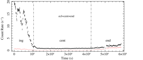
Figure 1: Count rates from the MOS1 detector. We show the count rate from a source region in black and from a background in red. An increase at late time in both count rates is indicative of an increase in the non-X-ray background. Each data point represents the average count rate over 128 s. Time zero on the abscissa is 2001-05-31 02:22:16.9357 UT.

In the beginning, the count rate in the source region decreases through X-ray eclipse ingress. Toward the end of the observation, the count rates for both the source and the background regions increase while the difference stays approximately constant indicating an increase in the non-X-ray background. We divided the data into the three time intervals noted on the figure. On the time scale of the figure, the times which divide the intervals are 10609 s and 42289 s. The intervals, labeled “ingress”, “center”, and “end” were chosen to divide the eclipse ingress from the time of complete X-ray eclipse and the time of high background from the rest of the observation. We then extracted spectra from each of the five XMM-Newton X-ray instruments for each of the three intervals and from the interval consisting of the center and end intervals which we label “eclipse”.

We focus here on the spectral data from the RGS. However, in Figure 2 we plot the spectrum from MOS 1 for the eclipse interval.

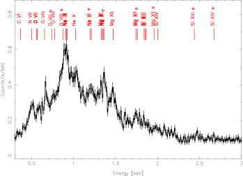
Figure 2: MOS 1 Eclipse spectrum of SMC X-1. Labels indicate the energies of spectral features which may or may not be detected in this spectrum. The labels denote the energies of lines except where the ion is followed by “e” indicating an edge. The line energies indicated are $n=2\to 1$ transitions except for 0 VIII at 0.77 keV, Ne X at 1.21 keV, and Mg XII at 1.74 keV which are $n=3\to 1$ transitions.

This spectrum is similar to those spectra of SMC X-1 obtained by Vrtilek et al. (2001) with Chandra/ACIS. In Figure 3 we show our RGS spectrum for the eclipse interval.

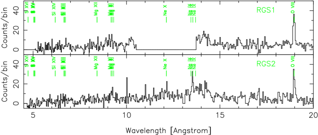
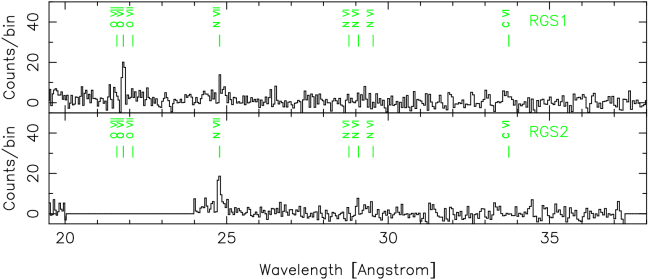
Figure 3: The RGS eclipse spectrum of SMC X-1.

Line emission from hydrogen-like and helium-like ions of several elements is apparent. The spectral resolution of the XMM-Newton RGS is such that the $n=2\to 1$ transitions of helium-like ions are resolved into a triplets consisting of, in order of wavelength, the resonance ($1s2p\,^{1}\!P_{1}\to$ground), intercombination ($1s2p\,^{3}\!P_{2,1}\to$ground), and forbidden ($1s2s\,^{3}\!S_{1}\to$ground) lines. However, in our RGS spectra, only the intercombination lines are apparent. Before attempting to explain this fact or to use it to derive constraints on the properties of the SMC X-1 system, we first make a quantitative characterization of the line emission.

In order to measure the fluxes, widths and shifts of these lines, we fit the wavelength channels within 0.5 Å of the rest wavelengths of each of the $n=2\to 1$ emission line complexes. We fit the spectrum in the vicinity of each line complex using a power law continuum and Gaussian lines. We express the width (sigma) and centroid of the Gaussians in velocity coordinates and fix the width and shifts of the lines in a single complex to be the same, i.e. :

$$F_{\lambda}=K(hc)^{\alpha+1}({\rm keV})^{\alpha}{}\lambda^{-(\alpha+2)}+\sum_{k}\frac{1}{\lambda_{k}(v_{r}/c)\sqrt{\pi}}I_{k}\exp\left(\frac{(\lambda-\lambda_{k}(1+v_{r}/c))^{2}}{2\lambda_{k}^{2}(\sigma_{v,r}/c)^{2}}\right)$$ (1)

where $F_{\lambda}$ is the photon (not energy) flux, the $\lambda_{k}$s are the rest wavelengths of the lines, and $K$, $\alpha$, $v_{r}$, $\sigma_{v,r}$, and the $I_{k}$s are fit parameters. We assume that lines appear in emission and therefore constrain the fluxes of all lines to be greater than or equal to zero.

The intercombination line is actually an unresolved doublet. Therefore, we fit the ingress and eclipse spectra in the vicinity of the helium-like triplets using the model described by equation 1 with four Gaussians: one for each of the resonance and forbidden lines and one for each of the two components of the intercombination line. However, we fix the ratio of the fluxes of the two components of the intercombination line to be equal to that predicted by Kinkhabwala et al. (2003) for recombination using temperatures given in Table 3.3. Furthermore, for reasons we describe later, we formulate our model not in terms of the individual fluxes of the three lines of the triplets but in terms of the total triplet line flux $I$ and the ratios of the line fluxes $G$ and $R$ where

$$G\equiv\frac{I_{\rm i}+I_{\rm f}}{I_{\rm r}}$$ (2)

and

$$R\equiv\frac{I_{\rm f}}{I_{\rm i}}$$ (3)

where the subscripts “r”, “i”, and “f” indicate, respectively, the resonance, intercombination, and forbidden lines. In the fits, we restrict the value of $\sigma_{v,r}$ to be less than 1500 km s^-1, $v_{r}$ to be between $-$1000 and 1000 km s^-1 and we restrict $I$, $G$, $R$, and $K$ to be greater than or equal to zero. In Figures 4 and 5,

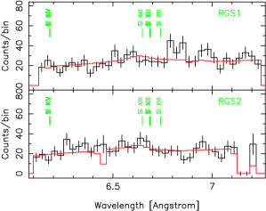
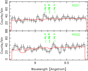
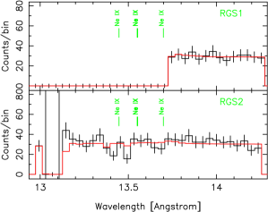
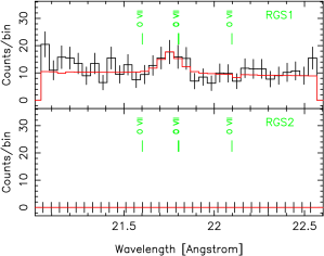
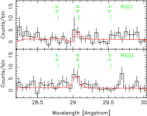
Figure 4: Helium-like triplets for the “ingress” interval.

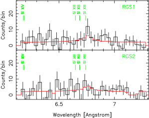
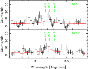
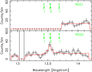
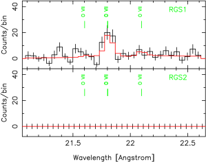
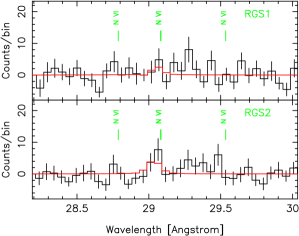
Figure 5: Helium-like triplets for the “eclipse” interval.

we show our best fits to these triplets and in Table 1 we show the best-fit values and confidence intervals for these line fluxes, shifts and widths. The fact that we detect only the intercombination lines of the helium-like triplets is reflected in the fact that we obtain only lower limits on $G$ and only upper limits on $R$.

Table 1: Measured Helium-like Triplet Parameters

						power-law
Element	$I$	$G$	$R$	$\sigma_{v,r}$(km s-1)	$v_{\rm r}$(km s-1)	K	$\alpha$
ingress
N	1.2${}^{+0.7}_{-0.6}$	$>$4	$\cdots$	$<$800	$-$300${}^{+400}_{-300}$	36${}^{+10}_{-36}$	0${}^{+\infty}_{-2}$
O	2.6${}^{+1.4}_{-1.5}$	$>$3	$<$0.3	500${}^{+600}_{-500}$	$-$500${}^{+600}_{-\infty}$	135${}^{+14}_{-111}$	0${}^{+\infty}_{-3}$
Ne	1.4${}^{+4.2}_{-1.4}$	$\cdots$	$\cdots$	$\cdots$	$\cdots$	170$\pm$30	$-$0.9${}^{+\infty}_{-2.0}$
Mg	2${}^{+6}_{-2}$	$\cdots$	$\cdots$	$\cdots$	$\cdots$	205${}^{+16}_{-50}$	$-$1.1${}^{+1.1}_{-0.3}$
Si	22${}^{+17}_{-16}$	$\cdots$	$\cdots$	$\cdots$	$\cdots$	280${}^{+90}_{-70}$	$-1.3\pm 0.5$
eclipse
N	0.22$\pm$0.18	$>$1.6	$<$0.63	$<$500	$-$400${}^{+500}_{-200}$	$<$1.3	$\cdots$
O	1.1$\pm$0.4	18${}^{+\infty}_{-14}$	0.26${}^{+0.34}_{-0.26}$	$<$300	90${}^{+130}_{-270}$	$<$0.0002	21.5${}^{+0.6}_{-13.6}$
Ne	1.8${}^{+0.7}_{-0.8}$	$>$9	0.2${}^{+0.3}_{-0.2}$	$<$600	$-$400${}^{+500}_{-300}$	6.5$\pm$0.7	-6${}^{+5}_{-\infty}$
Mg	2.2${}^{+0.9}_{-0.7}$	$>$2	$<$0.25	$<$1300	$-$600${}^{+600}_{-\infty}$	3.8${}^{+1863.5}_{-0.6}$	0${}^{+\infty}_{-3}$
Si	2.4${}^{+2.4}_{-2.0}$	$\cdots$	$\cdots$	$\cdots$	$\cdots$	2.5${}^{+1863.9}_{-0.8}$	0${}^{+\infty}_{-9}$

Note. — As a confidence limit on $\sigma_{v,r}$, $v_{\rm r}$, or $\alpha$, $\infty$ indicates that parameter boundaries are within the confidence limits. The entry “ $\cdots$ ” indicates that the data do not constrain this quantity.

The hydrogen-like $n=2\to 1$ transitions consist only of an unresolved doublet and we fit these doublets using two Gaussians with the ratio of the fluxes of those two lines fixed at 2:1, proportional to the statistical weights of the upper levels and the ratio expected for recombination. Furthermore, we restrict $\sigma_{v}$ to be less than 2500 km s^-1 and $v_{r}$ to be between $-$2500 and 2500 km s^-1. In Table 2, we show the fit parameters for the hydrogen-like lines. Again, $I$ indicates the total photon flux for the doublet.

Table 2: Measured Hydrogen-like Line parameters

				power-law
$Z$	$I$($10^{-6}$s-1cm-1)	$\sigma_{v,r}$(km s-1)	$v_{\rm r}$(km s-1)	norm	$\alpha$
ingress
6	0.5${}^{+0.6}_{-0.5}$	$\cdots$	$\cdots$	$<$1900	$\cdots$
7	1.0${}^{+0.7}_{-0.8}$	$<$1200	600${}^{+500}_{-1800}$	174${}^{+17}_{-159}$	0${}^{+\infty}_{-3}$
8	4${}^{+3}_{-2}$	900${}^{+1100}_{-900}$	$-$2300${}^{+900}_{-\infty}$	16${}^{+26}_{-13}$	$-$6${}^{+4}_{-\infty}$
10	7$\pm$5	2500${}^{+\infty}_{-2000}$	$\cdots$	171${}^{+14}_{-13}$	0.0${}^{+\infty}_{-1.8}$
12	1.4${}^{+9.4}_{-1.4}$	$\cdots$	$\cdots$	170$\pm$30	$-$0.4${}^{+\infty}_{-0.3}$
14	44${}^{+16}_{-22}$	$\cdots$	2000${}^{+\infty}_{-4000}$	29000${}^{+42000}_{-17000}$	$-$8.6${}^{+1.4}_{-1.2}$
eclipse
6	0.3$\pm$0.3	1300${}^{+\infty}_{-900}$	$-$1500${}^{+1900}_{-\infty}$	$<$8	$\cdots$
7	0.7$\pm$0.2	$<$400	0$\pm$200	9$\pm$3	$\cdots$
8	1.7$\pm$0.3	$<$400	160${}^{+70}_{-140}$	8.4$\pm$1.9	0${}^{+\infty}_{-3}$
10	1.0$\pm$0.6	$\cdots$	200${}^{+900}_{-1100}$	7.5$\pm$1.4	0${}^{+\infty}_{-5}$
12	0.9${}^{+1.0}_{-0.9}$	$\cdots$	$\cdots$	17${}^{+1892}_{-4}$	$\cdots$
14	$<$2.0	$\cdots$	$\cdots$	3.3${}^{+2632.6}_{-1.6}$	$\cdots$

Note. — The entry “ $\cdots$ ” indicates that the data do not constrain this quantity.

3 Line Fluxes as Measures of the Distribution of Scatters in Physical and Velocity Space

The emission lines from high-mass X-ray binaries result from recombination and resonant line scattering in wind of the high-mass star. The line emission from these processes depends on the distribution of the wind material in coordinate space and, in the case of resonant line scattering, in velocity space. Therefore, the line fluxes we measure provide a constraint on these distributions of the wind material. However, the equations that describe these distributions are complex and rather than attempt to derive constraints directly from the line fluxes, we believe it will be more illuminating to create a simple model described by a few parameters and then derive constraints on these parameters. In §3.1, we derive equations for line luminosities due to recombination and resonant line scattering. In §3.2, we describe a modification to those luminosities for the case of the helium-like triplets due to ultraviolet radiation of the high-mass star. In §3.3 we describe the simple models and our constraints on their parameters.

3.1 Recombination and Resonant Line Scattering

In a plasma in photoionization equilibrium, photons are absorbed from the continuum in photoionizing transitions and line photons are emitted as electrons and ions recombine. If the plasma is optically thin in the photoionizing continuum, the recombination line luminosity may be expressed as

$$L_{{\rm rec}}=h\nu_{0}\frac{\pi{}e^{2}}{m_{e}c}(4\pi)^{-1}\int\!\!\!\int\eta n_{{\rm Ion}}ds\,d\Omega\int_{\nu_{\rm th}}^{\infty}\frac{L_{\nu}}{4\pi{}h\nu}\frac{df}{d\nu}d\nu$$ (4)

where $h$ is Planck’s constant, $\nu_{0}$ is the frequency of the line, $e$ and $m_{e}$ are the electronic charge and mass, $n_{{\rm Ion}}$ is the density of the ion that emits the line, $\eta$ is fraction of recombinations to the ion which result in emission of the line, $L_{\nu}$ is the specific luminosity of the compact X-ray source, $\nu_{\rm th}$ is the ionization threshold frequency of the emitting ion in its ground state, and $df/d\nu$ is its continuum oscillator strength, and $s$ and $\Omega$ are the distance from and solid angle subtended at the compact X-ray source.

In any plasma, line photons are absorbed and reemitted in resonance line transitions. The net effect of this is only to redirect line photons. However, depending the geometry of the plasma and radiation source, resonant line scattering may result in absorption or emission lines being observed. For the geometry of interest in this work — an occulted compact radiation source with radiation scattered into the observer’s line of sight by plasma — resonant scattering results in emission lines and the line luminosity due to scattering may be expressed as

$$L_{{\rm scat}}=L_{\nu_{0}}(4\pi)^{-1}\int\!\!\!\int(1-e^{-\tau(\nu,{\bf\Omega})})d\nu{}d\Omega$$ (5)

where $\tau$ is the line optical depth through the plasma along a line from the compact radiation source. The line optical depth is given by

$$\tau=f\frac{\pi{}e^{2}}{m_{e}c}\int{}n_{\rm Ion}\phi(\nu)ds$$ (6)

where $f$ is the line oscillator strength and the function $\phi$ describes the line profile. Neglecting natural line broadening and considering only Doppler line broadening, we have

$$\phi(\nu)\equiv\frac{c}{\nu_{0}}g(c(\nu/\nu_{0}-1))$$ (7)

where $g$ is the local distribution of the ions’ velocity component in the direction along the line of sight from the compact X-ray source and is normalized such that

$$\int_{-\infty}^{\infty}g(v)dv\equiv 1.$$ (8)

However, we assume that ion velocities are very small compared to $c$ so that $g(v)$ is non-zero only for $|v|\ll{}c$. With this definition,

$$\int_{0}^{\infty}\phi(\nu)d\nu=1.$$ (9)

As we will ultimately be interested in calculating observed line fluxes the spatial integrals in equations 4 and 5 should be restricted to the volume that is both illuminated by the compact radiation source and observable (i.e., not occulted by the star). In principle, the radiation from the compact source that reaches the observable plasma may be depleted at the line frequency by line scattering in the occulted region, reducing the observable line luminosity relative to that described by equation 5. However, as scattering does not destroy photons but merely redirects them, for most plasma geometries, the total number of line photons reaching the observable region will not be significantly affected by scattering in the occulted region. Only for a specialized plasma geometry: a long, narrow distribution of plasma, oriented along a line of sight from the compact radiation source will equation 5 be significantly inaccurate. Furthermore, if the part of the wind where the line emission occurs is moving supersonically (as HMXB winds are known to do) the line frequencies in different parts of the wind will be shifted apart so that resonant line scattering in one part of the wind will not be affected by resonant line scattering in another part.

In equation 4, we have $\eta$ inside the spatial integral, allowing for the possibility that the recombination efficiencies may depend on the local conditions. In fact, for helium-like lines, the forbidden line may be “pumped” into the intercombination line at high densities or high ultraviolet radiation intensities and we define $\eta$ so that the effects of this pumping are absorbed into it. Near a hot star such as Sk 160, the B0 companion of SMC X-1, the ultraviolet radiation intensity is high. Therefore, the line luminosities due to resonant scattering depend on the distance from the star. In the next section, we describe this in more detail.

3.2 Helium-like Triplets

As can be seen from the equations above, the observed flux of any one line depends in a complicated way on the distribution of the emitting ions in both coordinate and velocity space. Therefore, the constraint that can be derived from a single line is quite complex. However, because the resonance line of each helium-like triplet has a significant oscillator strength while the other two lines do not, only the resonance line is affected by resonant scattering. Therefore, only the flux of the resonance line depends on the velocity distribution of the emitting ions and by measuring the flux of all three lines of the triplet, it is possible to derive more specific constraints on the distribution of the emitting ions in space and velocity than can be obtained from the flux of any one line.

As previously mentioned, the recombination efficiencies of the intercombination and forbidden lines are not constant but depend on the local conditions. This is due to the fact that the upper level of the forbidden line, the ${}^{3}S_{1}$ level, is metastable and an ion in that state may be excited by absorption of an ultraviolet photon or collision with an electron to any of the ${}^{3}P$ levels. Two of these levels (${}^{3}P_{2}$ and ${}^{3}P_{1}$) make up the upper levels of the intercombination line. Therefore, at high densities or high ultraviolet radiation intensities, the effective recombination efficiency of the intercombination line is increased and the effective recombination efficiency of the forbidden line is decreased. This effect has been used by several authors to estimate the distance of emitting ions from isolated hot stars. However, several of the calculations have neglected the fact that once an ion is excited from the ${}^{3}S_{1}$ state to a ${}^{3}P$ state, it may decay back to the ${}^{3}S_{1}$ state by emission of an ultraviolet photon rather than decay to ground by emission of an intercombination line photon. We write the recombination line efficiencies including this effect as

$$\eta_{\rm i} = \eta_{\rm i}^{\prime}+\eta_{\rm f}^{\prime}(1-b_{\rm f})$$ (10)

$$\eta_{\rm f} = \eta_{\rm f}^{\prime}{}b_{\rm f}$$ (11)

where $\eta_{\rm i}^{\prime}$ and $\eta_{\rm f}^{\prime}$ are the recombination efficiencies without ${}^{3}S_{1}\to{}^{3}P$ excitation and $b_{\rm f}$ is the branching ratio for radiative decay of the ${}^{3}S_{1}$ state to ground. In order to derive an expression for this branching ratio, we solve the rate equations of Mewe & Schrijver (1978, equations 18 and 19) and neglect inner-shell ionization, all collisions, and induced radiative decay. To write our expression, we use the notation of Porquet et al. (2001) and denote the ${}^{3}S_{1}$ level by $m$ (for “metastable”), the ground ($1s^{2}\,{}^{1}S_{0}$) by $g$ and denote the level ${}^{3}P_{k}$ by $p_{k}$ where $k$ may be 0, 1, or 2 and get

$$b_{\rm f}\equiv\frac{A_{mg}}{A_{mg}+T}$$ (12)

where

$$T\equiv\sum_{k=0}^{2}w_{mp_{k}}\frac{A_{p_{k}g}}{A_{p_{k}g}+A_{p_{k}m}}$$ (13)

where $w_{mp_{k}}$ is the excitation rate from the ${}^{3}S_{1}$ to ${}^{3}P_{k}$.

For photoexcitation, the $w$ values are given by

$$w_{mp_{k}}=\frac{4\pi{}^{2}e^{2}}{m_{e}c}f_{mp_{k}}\frac{J_{\nu_{mp_{k}}}}{h\nu_{mp_{k}}}$$ (14)

where $J_{\nu_{mp_{k}}}$ is the mean intensity of radiation (i.e., the intensity averaged over solid angle) at the frequency $\nu_{mp_{k}}$ and $\nu_{mp_{k}}$ and $f_{mp_{k}}$ are, respectively, the frequency and oscillator strength of the transition $m\to{}p_{k}$. The frequencies $\nu_{mp_{k}}$ for elements from carbon to iron range from the near to the extreme ultraviolet. Because the quantity $\eta_{\rm i}+\eta_{\rm f}$ and the value of $\eta_{\rm r}$ do not depend on the ultraviolet pumping, neither does the value of the $G$ ratio but the value of the $R$ ratio does.

3.3 Simple Model

From the observed fluxes of the three lines of a given helium-like triplet, it is possible to derive constraints on the distribution of the helium-like ions in coordinate and velocity space. However, because of the complexity of the equations describing the line luminosities, the constraints that can be derived are also complex. Therefore, we compute line fluxes for two simple parameterized models for the distribution of material. Then we derive constraints on those parameters from the observed line fluxes. We do not actually expect the distribution of material in the wind of SMC X-1 to be described by these simple models in detail. However, from these model parameter constraints it is possible to make approximate inferences about the distribution of the wind of SMC X-1 in coordinate and velocity space.

In our models, each ion exists exclusively within a solid angle $\Omega$ subtended at the neutron star, and is distributed such that the column density along lines of sight from the neutron star has the single value $N$ within the solid angle $\Omega$. The distribution of ion velocities along lines of sight from the neutron star in our model is uniform over some range with width $\Delta{}v$ (which need not be centered on zero). Also, to simplify the calculation of ultraviolet pumping, we take the entire plasma to be at a single distance $r$ from the surface of the companion star which we take to be a sphere emitting as a blackbody with a temperature of $T_{\star}=$30,000 K, the approximate effective temperature for a star of type B0 such as Sk 160.

For this model, the UV radiation density is

$$J_{\nu}=W(r)B_{\nu}(T_{\star})$$ (15)

where $B_{\nu}$ is the Planck function,

$$W(r)\equiv\frac{1}{2}\left[1-\left(1-\left(\frac{r_{\star}}{r}\right)^{2}\right)^{1/2}\right],$$ (16)

and $r_{\star}$ is the stellar radius. The luminosity of a line due to recombination is then

$$L_{{\rm rec}}=h\nu_{0}\frac{\pi{}e^{2}}{mc}(4\pi)^{-1}\eta\Omega{}N\int_{\nu_{\rm th}}^{\infty}\frac{L_{\nu}}{4\pi{}h\nu}\frac{df}{d\nu}d\nu$$ (17)

and the line luminosity due to scattering is

$$L_{{\rm scat}}=L_{\nu_{0}}(4\pi)^{-1}\frac{\nu_{0}}{c}\Omega\Delta{}v(1-e^{-f\frac{\pi{}e^{2}}{m\nu_{0}}\frac{N}{\Delta{}v}}).$$ (18)

or, equivalently,

$$L_{{\rm scat}}=L_{\nu_{0}}(4\pi)^{-1}\frac{\nu_{0}}{c}\Omega{}N\frac{1-e^{-f\frac{\pi{}e^{2}}{m\nu_{0}}\frac{N}{\Delta{}v}}}{N/\Delta{}v}.$$ (19)

It can be seen from the above expressions that it is not necessary to specify all of the model parameters in order to determine the line luminosities. It is sufficient to specify only the parameter combinations $\Omega{}N$ and $N/\Delta{}v$ rather than the values of the three parameters contained in those two combinations. If we replace the three parameters with the two parameter combinations then the fluxes of the lines depend linearly on $\Omega{}N$, the sum of the luminosities of the intercombination and forbidden lines depends only on $\Omega{}N$, the $G$ ratio depends only on $N/\Delta{}v$, and the $R$ ratio depends only on $r$.

In principle, it should be possible to derive constraints on the model parameters from the constraints on the line fluxes in Table 1. However, for the line emission mechanisms we consider here, the $G$ and $R$ ratios can only take on values within a finite range (e.g., see Wojdowski et al. 2003 Figure 8 for the range of the $G$ ratio for Si XIII). In at least one case, our best fit value of $G$ falls outside of this range. Therefore, in order to derive meaningful constraints on the physical model parameters, we redo the fits with the $G$ and $R$ values constrained to be within the range allowed by scattering and recombination as described above. In all cases, we are able to obtain good fits with these constraints imposed.

In order to relate our model parameters to line fluxes and derive constraints on our model parameters, we use the following data. We get recombination efficiencies (without ${}^{3}S_{1}\to^{3}P$ pumping) by dividing effective line recombination rates from Kinkhabwala et al. (2003) by total recombination rates from Verner et al. (1996). We have written equations for line luminosities in terms of the specific luminosity of the X-ray source. Of course, we measure fluxes and any luminosities we derive are subject to uncertainty in the distance to the object. However, if we write equations 4 and 5 in terms of fluxes, factors of distance cancel. Therefore, in our calculations we use fluxes and our results do not depend on the distance to SMC X-1. For the specific luminosity of the SMC X-1 neutron star $L_{\nu}$ we use

$${\cal F}=K\left(\frac{\epsilon}{1\,{\rm keV}}\right)^{-\alpha}$$ (20)

where ${\cal F}$ is the specific photon flux per unit photon energy interval which is related to $L_{\nu}$ by $L_{\nu}=(4\pi{}d^{2})^{-1}h^{2}\nu{\cal F}$ and $\epsilon$ is photon energy with $K=0.0267$ photons cm^-2 keV^-1 and $\alpha=1$ from a fit to the uneclipsed ASCA spectrum of SMC X-1 (Wojdowski et al., 2000). The value of 1 we use for $\alpha$ is an approximation to the best-fit value of 0.94$\pm$0.02. For the continuum oscillator strength of the helium-like ions above the ionization threshold we use

$$\frac{df}{d\nu}=2\nu_{\rm th}^{2}\nu^{-3}$$ (21)

(c.f., Wojdowski et al., 2003). For all elements, we take the oscillator strength of the resonance line to be 0.7, which is accurate to 5%. For line frequencies (wavelengths) and spontaneous decay rates we use values from the Astrophysical Plasma Emission Database (APED, Smith et al., 2001). We take the oscillator strengths $f_{mp_{0}}$ to be zero and derive the oscillator strengths $f_{mp_{1}}$ and $f_{mp_{2}}$ from the spontaneous deexcitation rates of APED. We give the results of our model parameter constraints in Table 3.3.

Table 3: Simple Model Parameters Derived from Helium-like Line Emission

element	$T_{\rm rec}$(eV)	$\Delta\tau$	$r/r_{\star}$	$N/\Delta{}v$	$\Omega(4\pi)^{-1}N$	$\Omega(4\pi)^{-1}\Delta{}v$	$T_{\rm rec}$
				($10^{15}$ cm-2(km s-1)-1)	($10^{15}$ cm-2)	(km s-1)	reference
N	3.0	$>$4.2	$<$57	$>1.0$	0.22$\pm$0.18	$<$0.39	1
O	4.0	$>$20	18${}^{+11}_{-17}$	$>6.4$	1.3$\pm$0.4	$<$0.27	1
Ne	12	$>$22	$<$6.6	$>11$	2.2${}^{+0.9}_{-1.0}$	$<$0.27	2
Mg	21	$>$4.2	$<$1.4	$>3.2$	3.4${}^{+1.4}_{-1.1}$	$<$1.5	2
Si	75	$\cdots$	$\cdots$	5.1${}^{+5.1}_{-4.2}$	$\cdots$	$\cdots$	2

References. — (1) Kinkhabwala et al. 2003; (2) Sako et al. 1999

4 Summary/Discussion

We have observed SMC X-1 in eclipse with XMM-Newton and, with the RGS, resolved the helium-like triplets of nitrogen, oxygen, neon, and magnesium. To our knowledge, this is the first time helium-like triplets from SMC X-1 have been resolved and the first time the helium-like triplets of nitrogen, oxygen, or neon have been resolved for any HMXB. In all cases, only one component of the triplet, the intercombination line, is observably present. The lack of observable forbidden line fluxes in the triplet is easily explained by photoexcitation pumping of the forbidden line into the intercombination line by the ultraviolet radiation of the B0 star Sk 160 and allows upper limits to be set on distance of the emitting helium-like ions from Sk 160. The absence of observable fluxes in the resonance lines is consistent with what we expect from recombination in the photoionized wind. However, the fact that the resonance lines are not enhanced by resonant scattering implies a lower limit on the optical depth of the wind in the resonance line and, therefore, constraints on the structure and kinematics of the wind are also implied.

We have modeled the helium-like line emission as recombination and scattering emission from a region that is partly obscured by the companion star and is described by a single solid angle ($\Omega$) and column density ($N$) and the velocities along lines of sight from the neutron star have a boxcar distribution with width $\Delta{}v$ for each of the ions. We have inferred infer the quantity $\Omega\Delta{}N$ from the sum of the flux of the intercombination and forbidden lines which are not affected by resonant line scattering. We infer the quantity $N/\Delta{}v$ from flux of the resonance line relative to the sum of the other two (the inverse of the $G$ ratio). From the constraints on these two quantities, we also obtain a constraint on the quantity $\Omega\Delta{}v$. Because we do not detect the resonance line, we obtain only lower limits on $N/\Delta{}v$ and only upper limits on $\Omega{}\Delta{}v$.

As previously mentioned, in our analysis we have assumed that photons escape isotropically along lines from the location of their production or first scattering. While we do expect recombination emission to be isotropic, resonant line scattering is not isotropic. The angular distribution for resonant line scattering is a linear combination of an isotropic distribution and an dipole distribution (see, e.g., Chandrasekhar, 1960, Ch. 19). Furthermore, for large optical depths that are comparable to or greater than unity such as we infer, photons may undergo several scatterings before escaping. In this case, photons will escape preferentially along directions where the optical depth is least. In general, the calculation of photon escape direction is also complicated by the fact that photons may travel large distances across the plasma before escaping. While it is difficult to include this possibility in analytic calculations, it is straightforward using Monte Carlo techniques. However, if the region that emits the helium-like line emission has supersonic velocity differentials, as we know that the bulk of the wind does, the transfer of resonant line photons is essentially local (the Sobolev approximation, Castor 1970) and can be approached analytically. For a supersonically expanding wind, the optical depth in a direction given by the coordinate $x$ is inversely proportional to $dv_{x}/dx$. If the flow moves along lines from a single point and $y$ is the distance from that point, then these derivatives, in directions parallel and perpendicular to the flow, respectively, are $dv/dy$ and $v/y$. While these quantities will not generally be equal, they will generally be of the same order over the bulk of the wind and, therefore, if we assume complete redistribution in frequency and direction for individual scatterings, then the radiation will escape isotropically (see Castor, 1970). In fact, individual scattering events do not redistribute frequency and direction completely and so even with $v/s=dv/ds$, radiation does not escape isotropically. However the difference from the case of complete redistribution is no greater than 10%–20% (Caroff et al. 1972, see also Mihalas 1980). In light of these facts, we proceed to explore the implications of our results. However, it must be kept in mind that the approximations we have made for the radiative line transfer may quantitatively affect our conclusions.

The implication of our results on fundamental wind parameters, such as the mass-loss rate and the terminal wind velocity, is complex owing to factors such as the complex dependence of the ion fractions on density in photoionization balance. Therefore, interpreting these results in terms of fundamental wind parameters is difficult to do without computing line fluxes for complete wind models which is beyond the scope of this work. However, the upper limits on $(\Omega/4\pi)\Delta{}v$ that we obtain, approximately 1 km s^-1, are quite small compared to 1000 km s^-1, the order of the terminal wind velocities of massive stars and the wind velocity in a simulation of the wind of SMC X-1 by Blondin & Woo (1995). Therefore, the part of the wind that emits the helium-like lines cannot be homogeneously distributed around the entire wind. Instead, we believe that our results indicate either that the volume (or volumes) containing the helium-like ions of the various elements subtend a small solid angle at the neutron star or that the helium-like ions exist primarily in a region where the wind is at a small fraction of its terminal velocity or, perhaps, some combination of both.

One possible explanation of our results is that the helium-like ions exist primarily in dense clumps throughout the wind. Dense clumps in the wind of an HMXB have previously been invoked in the case of Vela X-1 by Sako et al. (1999) in order to explain the strong fluorescence lines observed from that system. Another possible explanation is that helium-like ions exist mainly near the surface of the star where the density is higher, the ionization less, and the velocity lower than in the outer parts of the wind (see, e.g., Liedahl et al., 2001). Furthermore, the part of a volume along the surface of the companion star with a thickness significantly less than one stellar radius that is visible during eclipse would subtend a solid angle significantly less than $4\pi$ from the neutron star. In Figure 6 we illustrate both of these possibilities.

Figure 6: In this figure we illustrate to possible distributions of the helium-like ions consistent with the helium-like line fluxes we measure. In the first panel we illustrate the possibility that the helium-like ions are in clumps distributed throughout the wind. In the second panel we illustrate the possibility that the helium-like ions are near the surface of the companion star.

Definitive tests of these hypotheses would require calculations of the line emission from detailed wind models and that is beyond the scope of this work. However, we expect that our results, including the remarkably small values of $\Omega\Delta{}v$ are consistent with current expectations about the nature of winds in HMXBs.

References

- Blondin (1994) Blondin, J. M. 1994, ApJ, 435, 756
- Blondin & Woo (1995) Blondin, J. M. & Woo, J. W. 1995, ApJ, 445, 889
- Blumenthal et al. (1972) Blumenthal, G. R., Drake, G. W. F., & Tucker, W. H. 1972, ApJ, 172, 205
- Caroff et al. (1972) Caroff, L. J., Noerdlinger, P. D., & Scargle, J. D. 1972, ApJ, 176, 439
- Castor (1970) Castor, J. I. 1970, MNRAS, 149, 111
- Chandrasekhar (1960) Chandrasekhar, S. 1960, Radiative Transfer (New York, NY: Dover Publications, Inc.)
- Kinkhabwala et al. (2003) Kinkhabwala, A., Behar, E., Sako, M., Gu, M. F., Kahn, S. M., & Paerels, F. B. S. 2003, ApJ, submitted, astro-ph/0304332
- Liedahl et al. (2001) Liedahl, D. A., Wojdowski, P. S., Jimenez-Garate, M. A., & Sako, M. 2001, in ASP Conf. Ser. 247: Spectroscopic Challenges of Photoionized Plasmas, 417, astro-ph/0105084
- Mewe & Schrijver (1978) Mewe, R. & Schrijver, J. 1978, A&A, 65, 99
- Mihalas (1980) Mihalas, D. 1980, ApJ, 238, 1034
- Porquet et al. (2001) Porquet, D., Mewe, R., Dubau, J., Raassen, A. J. J., & Kaastra, J. S. 2001, A&A, 376, 1113
- Sako et al. (1999) Sako, M., Liedahl, D. A., Kahn, S. M., & Paerels, F. 1999, ApJ, 525, 921
- Smith et al. (2001) Smith, R. K., Brickhouse, N. S., Liedahl, D. A., & Raymond, J. C. 2001, ApJ, 556, L91
- Verner et al. (1996) Verner, D. A., Ferland, G. J., Korista, K. T., & Yakovlev, D. G. 1996, ApJ, 465, 487
- Vrtilek et al. (2001) Vrtilek, S. D., Raymond, J. C., Boroson, B., Kallman, T., Quaintrell, H., & McCray, R. 2001, ApJ, 563, L139
- Wojdowski et al. (2000) Wojdowski, P. S., Clark, G. W., & Kallman, T. R. 2000, ApJ, 541, 963
- Wojdowski et al. (2003) Wojdowski, P. S., Liedahl, D. A., Sako, M., Kahn, S. M., & Paerels, F. 2003, ApJ, 582, 959