Abstract

Many illnesses are associated with an alteration of the immune system homeostasis due to a combination of factors, including exogenous bacterial insult, endogenous breakdown (e.g., development of a disease that results in immuno suppression), or an exogenous hit like surgery that simultaneously alters immune responsiveness and provides access to bacteria, or genetic disorder. We conjecture that, as a consequence of the co-evolution of the human immune system with the ecology of pathogens, the homeostasis of the immune system requires the influx of pathogens. This allows the immune system to keep the ever-present pathogens under control and to react and adjust fast to bursts of infections. We construct the simplest and most general system of rate equations which describes the dynamics of five compartments: healthy cells, altered cells, adaptive and innate immune cells, and pathogens. We study four regimes obtained with or without auto-immune disorder and with or without spontaneous proliferation of infected cells. For each of the four regimes, the phase space is always characterized by four (but not necessary identical) coexisting stationary structurally stable states. Over all four regimes among the $4\times 4$ possibilities, there are only seven different states that are naturally described by the model: (i) strong healthy immune system, (ii) healthy organism with evanescent immune cells, (iii) chronic infections, (iv) strong infections, (v) cancer, (vi) critically ill state and (vii) death. Our description provides a natural framework for describing the relationships and transitions between these seven states. The analysis of stability conditions demonstrates that these seven states depend on the balance between the robustness of the immune system and the influx of pathogens. In particular, the healthy state A is found to exist only under the influence of a sufficiently large pathogen flux, which suggests that health is not the absence of pathogens, but rather a strong ability to find balance by counteracting any pathogen attack.

1 Introduction and general background

Our goal is to develop a model of a biological organism, defined as the collection of organs, tissues, cells, molecules involved in the reaction of the body against damaging stressors, which can take the form of (i) foreign biological material, (ii) damaged, aging and/or aggressive inner biological material and (iii) inorganic substances.

In a first broad-brush approach, the occurrence of illness is usually attributed to the following factors, which often act in combination, sometimes synergistically.

1. Microorganisms (bacteries, viruses, fungi, parasites) and the more recent extensions to prions. This reflects the germ theory of diseases which states that many diseases are caused by microorganisms, and that microorganisms grow by reproduction at the expense of the host, rather than diseases being spontaneously generated. We refer to the microbial origin of diseases as one of the “exogenous” insults to which the body is subjected.

2. Exogenous accumulative load of stressors in the environment, over-work, over-eating and other excesses, psychological and emotional factors (anger, fear, sadness, and so on) may lead to fatigue and/or epigenetic expressions. These various stressors impact the immune system by destabilizing the feedback processes of the cell-cell communication paths known to exist for the immune system: direct interaction with neighbor or self (juxtacrine and autocrine, respectively), short distances (paracrine, such as neurotransmitters), long distance endocrine (via hormones) and long distance nerves (such as vagus nerve).

3. Genetic variation (which include polymorphisms that affect outcome, as well as “disorders” or mutations, per se) caused by an unwelcomed mutation as in cancers, by the accidental duplication of a chromosome, or the defective genes inherited from the person’s parents (hereditary disease). One should distinguish between two types of hereditary diseases, those that are immuno-genetic diseases and immune disorders. The former are the expression of a major immune disfunction (as for example in trisomy 21 or the Turner syndrome) or of the deficiency of an enzyme essential to life (such as in mucoviscidosies, leucodystrophies, Wilson disease, and so on). These affections are triggered within the first few months of life and, for most of them, are life-threatening. The only treatment, which is at its beginnings, consists in gene transfer via a viral vector. In contrast, acquired immune disorders appear later, often during adult life. These diseases frequently are expressing defects affecting those parts coding the immune system in the region HLA of chromosome 6. At present, more than 45 auto-immune illnesses have been linked to the idiosynchratic characteristics of this region. We refer to the genetic disorder origin of diseases as “structural” and the present model offers a relevant framework.

4. Senescence, engineered death (cells “wear out”).

Most changes that occur in response to stimuli are adaptive, allowing the system to return back to its “attractor” state, often referred to as homeostasis. Damaging responses can result from host failure, overwhelming stimulus, or a combination of the two, and as a consequence, the host state may then not return to the original attractor, perhaps a new (different) attractor/state. A normal system may encounter an overwhelming stimulus (e.g., sepsis). Rarer occurrence in everyday life are the transient and partial failure of the immune system which may lead to various degrees of inappropriate response: (i) different hypersensitivities, in which the system responds inappropriately to harmless compounds (allergies and intolerances), (ii) autoimmunity, in which the immune system (mainly via its antibodies) attacks its own tissues, e.g., systemic lupus erythematosus, rheumatoid arthritis, chronic lymphocytic thyroiditis and myasthenia gravis, (iii) immunodeficiency, in which parts of the immune system fail to provide an adequate response (an example of failure to respond is cancer, in which the immune system fails to recognize the tumoral cells as dangerous).

Our hypothesis developed below in the mathematical model is based on the recognition that the human body and immune system function in a form of homeostasis, a dynamical equilibrium whose balance is continuously subjected to various external and internal stresses. Genuine epidemic diseases are relatively rare compared with illnesses that can be attributed to the transition of the homeostasis to an unbalanced state. Thus, given that the absence of illness, defined as health, is a form of homeostasis, living organisms regulate their internal environment so as to maintain a stable condition, by means of multiple dynamic equilibrium adjustments controlled by inter-related mechanisms of regulation. Main examples of homeostasis in mammals include the regulation of the amounts of water and minerals in the body by osmoregulation happening in the kidneys, the removal of metabolic waste by excretion performed by excretory organs such as the kidneys and lungs, the regulation of body temperature mainly done by the skin, the regulation of blood glucose level, mainly done by the liver and the insulin secreted by the pancreas. The mechanism of homeostasis is mostly negative feedback, according to which a system responds in such a way as to reverse the direction of change. There are also positive feedback systems, although they are apparently less frequent (for example, uterine contractions during parturition). But in contrast with other homeostatic systems, the immune system is probably better described by the fact that “The system never settles down to a steady-state, but rather, constantly changes with local flare ups and storms, and with periods of relative quiescence,” as expressed in the mathematical models developed in (Perelson, 2002; Perelson and Weisbuch, 1997; Nelson and Perelson, 2002). Our proposed model sees these “flares and storms” as transient nonlinear adjustments to fluctuating exogenous fluxes. We delay to a sequel paper the analysis of the dynamics of our mathematical system under the influence of time varying pathogen fluxes and under varying conditions. Here, we construct the model based on general concepts, and classify all its equilibrium states, each of them associated with a large class of affections.

The paper is organized as follows. Section 2 articulates our endogenous versus exogenous hypothesis, motivating the construction of the model presented in section 3. Section 3.1 gives the general mathematical framework in terms of nonlinear kinetic equations of the concentrations of five different classes of cells (or biological compartments). Section 3.2 specifies the kinetic rates of each elementary interaction between these five species of cells leading to the general form of the equations given in Section 3.3. Section 3.4 provides their dimensionless reduced form and section 3.5 presents our a priori expectations on the behavior of this model. Section 4 (respectively 5) presents the properties of the equilibrium states found when infected cells are not reproducing (respectively are reproducing) by themselves. Section 6 concludes. The Appendix presents the Lyapunov stability analysis around the fixed points.

2 Hypothesis of endogenous versus exogenous origins of diseases

The human immune system is subjected to incessant “attacks” by antigens of many different forms. Here, we use the term “antigen” to refer to all substances which are recognized as “non-self” endowed with an antigenic functionality, which includes pathogens, cell debris as well as toxins. A typical human being carries about $10^{14}$ bacteria (of course many of them symbiotic) and probably many more viruses. In comparison, the number of cells constituting the self is only about $10^{13}$ (ten trillions). In this context, the immune system is constantly challenged, it is performing a continuing “fight” and adaptation to ensure the integrity of the body. This can be viewed as a continuous flux of “small” perturbations to which the immune system has learned to adapt and to more or less cope with (Mazmanian et al., 2005; Palmer et al., 2007). Most of the time, an individual is in good health.

A first scenario is that a normal system may encounter an unusually strong insult leading to a disease. This is the most generally accepted scenario. As an example, consider the extreme case of a healthy human landing in the middle of a virulent cholera epidemic in Africa or sustaining severe injury in a car crash. We refer to this situation as an “exogenous” shock as the immune system has suddenly to cope with a serious attack from the corresponding pathogens or physical destructions.

Let us now consider a second hypothetical scenario, which we call “endogenous.” With the same typical fluxes of antigens, by stress or other destabilization external influences, or simply by chance, sometimes the immune system of an individual wanes and he becomes sick. This can occur after some fatigue (overwork, bad eating, stress, pain, psychological effects, and so on). In such a case, we cannot say that the illness is really due to a specific microbial attack, the microbes have been already present before; it is only that the immune system has gone a bit down. Perhaps, a succession of small random perturbations may add “coherently” in an unlucky run of random occurrences and lead to sickness, as suggested by system models of other complex systems (Sornette and Helmstetter, 2003; Sornette et al., 2003, 2004; Sornette, 2005). A given disease may have several completely distinct origins, e.g., liver cirrhosis which can be due to chronic viral infection, alcoholism, eating excesses (NASH, Non- Alcoholic Steatorrhoeic Hepatitis) or auto-immunity. Often, the revealed sickness could also be viewed as a positive, i.e., robust response (via inflammation, fever) to an invading organism. The perception of being ill and the need for rest may be adaptive and part of the overall dynamical response towards homeostasis. We refer to this class of events in which the immune system homeostasis is perturbed away from its domain of dynamical balance as an endogenously generated illness.

We are aware that this definition of “endogenous” may appear fuzzy, as a result of the many possible variations. If we have to be blunt, endogenous is everything that is not exogenous! Previous works have found specific dynamical diagnostics of endogenous evolution versus exogenous shock (Sornette and Helmstetter, 2003; Sornette et al., 2003, 2004; Sornette, 2005), which we will not pursue here as our emphasis is in the classification of the different homeostatic equilibrium states. We will defer to a future work for the dynamical aspects of the model.

We do not address here aging which also leads to failing immunity, as it is associated with a slow secular non-stationary state whose effect we neglect for time scales shorter than the average lifetime. Indeed, even the slow development of chronic diseases found in our model classification occurs over times scales of no more than a few decades and can thus be (marginally) separated from aging per se.

Based on these observations, our hypothesis is that a fundamental understanding of health, of illnesses, and of the immune system, requires an approach based on the concept of a self-organization of the immune system into a homeostasis under the continuous flux of external influences. We propose that many of the illnesses carried by humans are in significant part endogenous in nature and that, in order to understand the response of a human immune system to exogenous shocks, it is necessary to understand its endogenous organization and the fact that spontaneous fluctuations in the dynamics of the immune system will occur as a result of many coherently interfering factors, which may lead to any of a variety of pathological states mentioned above. We propose to go beyond the exogenous-environmental-structural origins of illnesses summarized in the introductory section, to encompass a complex system approach in which the human immune system and the whole body are regulated endogenously under the influence of a continuous and intermittent flux of perturbations. We conjecture that, if the regulatory immune system was not constantly subjected to antigens, it would probably decay in part and the defense would go down as its adaptive part would not be sustained, thus becoming vulnerable to future bursts of pathogen fluxes. Thus, we claim that the correct point of reference is not to consider a microbe-free or gene-defect-free body, but a homeostatic immune system within a homeostatic body, under the impact of many fluxes, in particular fluxes of pathogens and of stresses taking many of the forms mentioned above. An analogy may serve to illustrate our point: consider the fate of the bones and muscles of a typical individual, which need to be continuously under the influence of a suitable gravity field, i.e., under stress (in the mechanical sense of the term!). Otherwise, as demonstrated by astronauts under zero-G, loss of bone and muscle, cardiovascular deconditioning, loss of red blood cells and plasma, possible compromise of the immune system, and finally, an inappropriate interpretation of otolith system signals all occur, with no appropriate counter-measures yet known (Young, 1999).

We conjecture that the healthy individual has a homeostatic immune system working at a robust level of stability, allowing it (1) to keep ever present pathogens under control and (2) to react and adjust fast to new infections and other stresses. Under such fluxes, the complex regulatory immune systems exhibit spontaneous fluctuations and shocks, in the form of illnesses, which are themselves modulated by other factors. In other words, we propose to view illnesses as emergent properties of a complex interplay and balance between the immune system, the pathogens and the other stress factors. We hypothesize that the emergent properties of the normal system (health) are different from those of the damaged system (disease). Recent works on other complex systems suggest that there are ways to find specific diagnostics distinguishing between endogenous and exogenous causes of crises and to derive precursors and possible remedies (Sornette and Helmstetter, 2003; Sornette et al., 2003, 2004: Sornette, 2005). Our hypothesis of an endogenous origin of illnesses resonates with the recent proposal that the adaptive immune system may have evolved in vertebrates to recognize and manage the complex communities of coevolved bacteria (McFall-Ngai, 2007): more than 2000 bacterial species have been found to be typically associated as partners to a human immune system, compared with fewer than 100 species of identified human bacterial pathogens, with exposure to them that are rare and transient.

Our endo-exo hypothesis extends the “hygiene hypothesis” (Strachan, 1989), which states that modern medicine and sanitation may give rise to an under-stimulated and subsequently overactive immune system that is responsible for high incidences of immune-related ailments such as allergy and autoimmune disease. Strachan (1989) thus proposed that infections and unhygienic contact might confer protection against the development of allergic illnesses. Researchers in the fields of epidemiology, clinical science, and immunology are now exploring the role of overt viral and bacterial infections, the significance of environmental exposure to microbial compounds, and the effect of both on underlying responses of the innate and adaptive immunity (Schaub, 2006). Bollinger et al. (2007) has recently suggested that the hygiene hypothesis may explain the increased rate of appendicitis ($\sim 6\%$ incidence) in industrialized countries, in view of the important immune-related function of the appendix. Our endo-exo hypothesis is also a distinct generalization of Blaser and Kirschner (2007)’s proposal that microbial persistent relationships with human hosts represent a co-evolved series of nested equilibria, operating simultaneously at multiple scales, to achieve an overall homeostasis. Blaser and Kirschner (2007) emphasize the maintenance of persistent host-adapted infections via ESS (Evolutionary Stable Strategies, a subset of Nash equilibria in game theory) played by different pathogens between themselves and the host selected for human-adapted microbes. In contrast, we emphasize the co-evolution of the immune system and the pathogens as a key element to ensure a stable and robust homeostasis.

The next section presents a model which embodies these ideas in the simplest possible framework, that of kinetic reactions occurring between five different types of cells. The interactions between these five compartments are thought to be the outcome of the co-evolution between the organism, its immune system and the pathogens. However, it is not the purpose of our model to describe this evolution, since the time scales modeled here are typical of the recovery times following pathogen insults, which are much shorter than those involved in evolution.

As reviewed by Louzoun (2007), mathematical models used in immunology and their scope have changed drastically in the past 10 years. With the advent of high-throughput methods, genomic data, and explosive computing power, immunological modeling now uses high-dimensional computational models with many (hundreds or thousands of coupled ordinary differential equations (ODEs)) or Monte Carlo simulations of molecular-based approaches. Here, in contrast, we develop a five-dimensional system of the coupled normal cells-immune system(s)-infected cells-pathogens, which is a direct descendent of the classical models that were based on simple ODEs, difference equations, and cellular automata. While the classical models focused on the simpler dynamics obtained between a very small number (typically two or three) of reagent types (e.g. one type of receptor and one type of antigen or two T-cell populations) (Louzoun, 2007), we are more ambitious with the goal of framing an holistic approach to the homeostasis of the immune system(s) seen to be continuously interacting with other compartments of the organism and with pathogens. Our motto is well-captured by the quote from the biocyberneticist Ludwig von Bertalanffy: “Over-simplifications, progressively corrected in subsequent development, are the most potent or indeed the only means toward conceptual mastery of nature.” We believe that, notwithstanding the development of large-scale computer intensive models, there is still and there will always be the need for simpler approaches. Any knowledge should be seen as the collection of a hierarchy of descriptions, from the more general level with few variables and fluxes, which like a cartoon provides an outline of the main traits of the portrait, to the more detailed microscopic approaches. In between, a series of intermediate levels form the bridges between the two extreme modeling levels. Examples are found in all sciences. For instance, in hydrodynamics, going from the micro- to the macro-scales, we have the micro-level of molecular dynamics, the density functional approaches, the Master equations, the Fokker-Planck equations and finally the Navier-Stokes equation at the largest coarse-grained scale. The coarse-graining approach to modeling is based either on averaging the micro-dynamics or (and this is the route followed here) by using a “Landau” approach based on symmetry and conservation laws that allows us to identify the leading variables and their interactions. As is well-known in statistical physics, this approach may introduce new terms that cannot be a priori predicted from the microscopic biological level, and which account in an effective emergent way for the many complicated pathways of interactions. It would be a fundamental mistake to expect that all terms can be explained or justified at the microscopic level. At a higher level, new terms and novel effective interactions should be expected (Anderson, 1972).

In the sequel, we start from a simple but already rather rich framework, that will provide a guideline for subsequent developments.

3 Mathematical formulation of the homeostasis dynamical processes associated with the immune system

3.1 General formulation

In order to formulate mathematically the various interactions between cells and pathogens, we resort to the method of rate equations. The method of rate equations is commonly employed for characterizing the evolution of competing species. The general description of this approach can be found in the book by Hofbauer and Sigmund (2002). In the rate-equation approach, one considers the average properties of a system and its constituents, with the averaging assumed to be done over the whole body. Therefore, the spatial structure of the latter can be arbitrary.

Our model can be viewed as a significant extension of simple two-dimensional models of viral infection involving just normal cells with population $N_{1}$ and altered cells with population number $N_{2}$. One of the simplest representative of this family reads (Nowak, 2006)

$${dN_{1}\over dt} = k-uN_{1}-bN_{1}N_{2}\;,$$ (1)

$${dN_{2}\over dt} = bN_{1}N_{2}-(u+v)N_{2}~{},$$ (2)

where $N_{1}$ (resp. $N_{2}$) is the number of normal (resp. infected) cells. The parameter $k$ represents the birth flux of normal cell, $u$ is their normal death rate and the last term $-bN_{1}N_{2}$ in the first equation is the rate of infection of normal cells when they come in contact with altered cells. The destruction term for the population $N_{1}$ is a creation term for the population $N_{2}$. The last term $-(u+v)N_{2}$ in the second equation with $v>0$ embodies the increased mortality rate due to the alteration. This model is sufficient to represent simple infection diseases, with a competant immune system in the presence of circulating germs.

However, there is much more to the immune system dynamics than just its response to external pathogens. The immune system is a complex network of interacting components which also evolve and change, accumulating history-dependent characteristics, properties, strengths and deficiencies. Specifically, a useful model of the immune system should be able to include in a single framework the four main classes of clinical affections: allergies, chronic infections, auto-immune diseases and cancers. The model we discuss below aims at presenting a coherent system view of these different affections.

We consider five different agents constituting a living organism. These are:

(i)

normal healthy cells, whose number will be denoted by $N_{1}$;

(ii)

altered, or infected, cells, whose number is $N_{2}$;

(iii)

adaptive, or specific, immune cells, quantified by the number $N_{3}$;

(iv)

innate, or nonspecific, immune cells, with the number $N_{4}$;

(v)

pathogens, their number being $N_{5}$.

The non-specific immune response includes polynucleus cells, pro-inflammatory enzymes and the complement system. The specific immune response includes the lymphocytes and their product antibodies. Dividing the immune response into two components comes at the cost of augmenting the complexity of the system, but seems necessary to capture how inflammation and other non-specific responses might lead to ill-adapted or even negative effects leading to feedbacks on the specific part of the immune system, possibly at the origin of allergies, chronic infections and auto-immune diseases. However, we use below a parametrization which allows one to combine the two components of the immune system into a single effective one, thus decreasing the complexity of the system to four coupled ODEs. Differentiating the specific interactions and differences between the two immune systems will be the subject of another study.

The dynamics of the agents described above, and their interactions, can be described similarly to those of other competing species in the models of population evolution, using a system of ODEs obeying the Markov property. The general rate equations for the competing species thus read

$$\frac{dN_{i}}{dt}=R_{i}N_{i}+F_{i}\;,$$

where $i=1,...,5$, $R_{i}$ are rate functions, and $F_{i}$ are external influxes. Rather than a constant incoming rate of normal cells as in (1), we use a proportional growth term $R_{1}N_{1}$, to emphasize the endogenous nature of the dynamics. Higher order nonlinear terms ensure saturation to a constant number of normal cells. In contrast, using a constant incoming rate of healthy cells relies on the existence of a reservoir, whose dynamics should not be kept exogenous since our goal is to provide a self-consistent classification of the different states of the immune system-pathogen complex.

The rate functions are dependent of the agent numbers, so that $R_{i}=R_{i}(N_{1},N_{2},N_{3},N_{4},N_{5})$. Also, both $R_{i}$ and $F_{i}$ can depend on time $t$. The rate functions, in general, can be modeled in different forms, having any kind of nonlinearity prescribed by the underlying process. The most often employed form for the rate functions, which we shall also use, is

$$R_{i}=A_{i}+\sum_{j}A_{ij}N_{j}\;,$$ (3)

which can be seen as a Taylor expansion in powers of the agent numbers. Since $A_{1}>0$ for the normal cells, the corresponding decay term $-A_{11}N_{1}^{2}$ is nonlinear. Both terms taken together make endogenous the homeostatic equilibrium of the normal cells, thus avoiding the need for an external source. As discussed below, except in the case of spontaneously proliferating infected cells, all other decay terms are otherwise linear.

Generally, we could include as well indirect interactions with higher-order nonlinearities in expression (3). For instance, the third-order terms $A_{ijk}N_{i}N_{j}N_{k}$ could be included. We do not consider such terms for two reasons. First, such indirect interactions are usually less important. Second, their influence, to a large extent, has already been taken into account by a combination of several second-order terms, such as $A_{ij}N_{i}N_{j}$. In the majority of cases, the above form of the rate equations is quite sufficient for catching the main features of the considered dynamics.

We are going to describe the leading processes and their associated equations for the main terms of the rate equations. These terms take into account all basic interactions between the constituents of a living organism. The discussed direct interactions yield the nonlinear terms of second order.

The structure of the kinetic equations must satisfy the following general rules:

(i) Same-order nonlinearities. Nonlinear terms, characterizing interactions between cells, have to be of the same order of nonlinearity.

(ii) Self-consistency of description. Equations include the major processes between cells. All interaction parameters are to be treated on the same footing. The modulation of these parameters by secondary processes must be either taken into account everywhere or neglected everywhere.

(iii) Action-counteraction dichotomy. Each process $A_{ij}N_{i}N_{j}$, representing the interaction between an $i$-cell with a $j$-cell, must have its counterpart process $A_{ji}N_{j}N_{i}$ (with $A_{ji}$ not necessarily opposite to $A_{ij}$).

3.2 Specific determination of the kinetic rates

3.2.1 Kinetics of healthy cells $N_{1}$

(1) Healthy cells die with a natural decay rate and they are also produced by a specialized system of cells. The net (total) linear rate of death-birth of healthy cells is $A_{1}$ and the corresponding term is $A_{1}N_{1}$.

(2) The decay of healthy cells is described by the nonlinear term $-A_{11}N_{1}^{2}$.

(3) The adaptive immune system occasionally attacks healthy cells, which provokes auto-immune diseases. This is described by the term $-A_{13}N_{1}N_{3}$.

(4) The innate immune system sometimes also attacks healthy cells (e.g. through inflammation), which is represented by the term $-A_{14}N_{1}N_{4}$.

(5) Healthy cells are infected by pathogens, a process given by the term $-A_{15}N_{1}N_{5}$.

3.2.2 Kinetics of infected (or anomalous) cells $N_{2}$

(1) Infected cells die with a natural rate $A_{2}$, hence the decay term $-A_{2}N_{2}$ with $A_{2}>0$. For $A_{2}>0$, i.e., such that the term $-A_{2}N_{2}$ corresponds to a net death quotient, infected cells cannot significantly duplicate themselves.

(1bis) It is also interesting to consider, the case where infected cells multiply with a net positive growth rate $|A_{2}|$ corresponding to choosing $A_{2}<0$. As the analysis will show, this will allow us to obtain states that can be interpreted as cancer afflictions. For instance, chronic inflammation (as in the case of stomach lining) can lead to cancer (Helicobacter pylori infection can lead to stomach ulcers short term and stomach cancer long term). We also use the terminology “cancer” loosely to refer to situations in which the multiplication of infected cells during chronic infections occurs as if it was a cancer according to a dynamic process similar to the cellular tumor growth.

(2) The decay process can include a nonlinear contribution with the term $-A_{22}N_{2}^{2}$ with $A_{22}\geq 0$.

(3) Infected cells are killed by the adaptive immune system, thus the term $-A_{23}N_{2}N_{3}$.

(4) They are also killed by the innate immune system, so the term $-A_{24}N_{2}N_{4}$.

(5) The natural decay rate of infected cells can be increased by interacting with pathogens, which implies the term $-A_{25}N_{2}N_{5}$.

(6) The number of ill cells increases by the infection of healthy cells by pathogens, which is represented by the term $A_{51}N_{5}N_{1}$.

3.2.3 Kinetics of the immune system

The immune system of vertebrates can be divided into the innate component (macrophages, neutrophils, and many types of proteins involved in inflammation responses) and the adaptive immune system (antibodies and lymphocytes B and T). These two components interact with each other, cooperating and regulating each other. Hormonal fluxes and the metabolism of fatty acids (precursors of prostaglandins with opposite effects) also play an important role in the regulation of pro- or anti-inflamatory signals. We thus specify the dynamics of the two immune system components as follows.

Recent research show that that ‘danger signals’, such as those found during viral infections, can be recognized by T and B cells of the adaptive immune system (Marsland et al., 2005a,b). It was generally considered that such sensing of ‘danger signals’ was limited to cells of the innate immune system. The fact that T cells have evolved to recognize ’danger signals’ opens a wide spectrum of possibilities including novel mechanisms for the maintenance of immune memory, the development of autoimmunity and general T cell homeostasis. We take into account this phenomenon in our description of the activation of the immune cells.

Kinetics of the adaptive immune system $N_{3}$

(1) Immune cells in the adaptive immune system die by apoptosis, which is described by the term $-A_{3}N_{3}$.

(2) For generality, the nonlinear decay, with the term $-A_{33}N_{3}^{2}$ is included, though it may be subdominant.

(3) The activity of immune cells is supported by healthy cells, whose part, the marrow, reproduces the immune cells; these processes are described by the term $A_{31}N_{3}N_{1}$.

(4) Adaptive immune cells are activated by infected cells, which gives the term $A_{32}N_{3}N_{2}$.

(5) The adaptive immune system can be inhibited by the innate part of the immune system, which corresponds to the term $-A_{34}N_{3}N_{4}$. For instance, allergic inflammation of the lung inhibits pulmonary antimicrobial host defense (Beisswenger et al., 2006). This process may be part of the control of the immune response after the removal of the infection or of the traumatism in order to avoid an auto-immune excess. More generally, overwhelming activation of innate immunity during sepsis produces profound, relatively long-lived depression of adaptive immunity, evidenced by sepsis-induced increased apoptosis of lymphocytes which decimates the population (Hotchkiss and Karl, 2003). Another, specific instance is the evolution of bacterial “escape mechanisms,” such as activation of innate immunity resulting in a cellular response that inhibits adaptive immunity. For example, macrophages infected with Mycobacterium tuberculosis secrete interleukin-6 which inhibits the response of neighboring (uninfected) macrophages to interferon-gamma (Nagabhushanam et al., 2003).

(6) Adaptive immune cells are activated by pathogens, implying the term $A_{35}N_{3}N_{5}$. In reality, the adaptive immune system is activated by antigen presenting cells, such as dendritic cells, macrophages, and other elements of the innate immune system. Because we would like to account for both the triggering as well as inhibitory effect of the innate immune system on the adaptive one, we have chosen to separate its actions, so that the activation is here proxied as if by a direct action of the pathogens, while the inhibition is explicitly written as the direct interaction $-A_{34}N_{3}N_{4}$ previously discussed.

Kinetics of the innate immune system $N_{4}$

(1) The natural decay is given by the term $-A_{4}N_{4}$.

(2) The decay can be increased by the nonlinear term $-A_{44}N_{4}^{2}$, which, though, may be quite small.

(3) The proliferation of immune cells, supported by healthy cells, is characterized by the term $A_{41}N_{4}N_{1}$.

(4) The activation by damaged cells gives the term $A_{42}N_{4}N_{2}$.

(5) The innate immune system can be activated by the adaptive part of this system, yielding the term $A_{43}N_{4}N_{3}$. At the biological level, this activation can proceed via feedback loops. The adaptive immune system secretes specific antibody (IgE in classical allergies, IgG4 for food intolerance). The complex AG-IgE (N4) activates mastocytes, which themselves liberate mediators of the non-specific inflammatory reaction (more than 300 proteases can be involved). The latter repress the specific immune system via the negative feedback of the Jayle cycle, leading to a deficit in antibodies, except for the IgE and/or IgG4, which induce a positive feedback towards a stronger inflammation response, via the degranulation of mastocytes and the attraction of the eosinophils.

(6) Pathogens activate the innate immune system, hence the term $A_{45}N_{4}N_{5}$.

3.2.4 Kinetics of pathogens (or allergens, chemical or ionised particles) $N_{5}$

(1) Pathogens have a finite lifetime, thus the existence of the term $-A_{5}N_{5}$, where $A_{5}$ is the “clearance rate” of the pathogens.

(2) In general, the nonlinear death (or elimination) term $-A_{55}N_{5}^{2}$ can also exist.

(3) By the action-counteraction principle that we follow for the coarse-grained description of the dynamics of the five compartments, the existence of the term $A_{25}N_{2}N_{5}$ in the equation determining the rate $dN_{2}/dt$ of change of the number of infected cells should be accompanied by a term $A_{52}N_{5}N_{2}$ entering in the equation for $dN_{5}/dt$. An attempt for a possible biological interpretation is as follows. When infected cells die by lysis catalyzed by the presence of pathogens, they release the pathogens they contained. A mass action description is then given by the term $A_{52}N_{5}N_{2}$. One could argue that the rate of production of pathogens due to lysis of infected cells should be better described by a term proportional to the number $N_{2}$ of infected cells, to the rate of lysis and to the number of infectious virus particles produced by the infected cell upon lysis. But consistent with our modeling strategy, we keep the above term $A_{52}N_{5}N_{2}$ as a coarse-grained description of how the interactions between the infected cells and the pathogens affect the dynamics of the later.

(4) Pathogens are killed by the adaptive immune system, giving the term $-A_{53}N_{5}N_{3}$.

(5) They are also killed or hindered by the innate immune system, leading to the term $-A_{54}N_{5}N_{4}$.

(6) There exists a continuous supply of pathogens into the organism from the exterior, represented by the influx $F$, which is, in general, time varying (but here we will take this flux constant in our analysis of stationary equilibrium states).

3.3 Kinetic equations

Summarizing the processes described above, we obtain the following system of kinetic equations

$$\frac{dN_{1}}{dt}=A_{1}N_{1}-A_{11}N_{1}^{2}-A_{13}N_{1}N_{3}-A_{14}N_{1}N_{4}-A_{15}N_{1}N_{5}\;,$$ (4)

$$\frac{dN_{2}}{dt}=-A_{2}N_{2}-A_{22}N_{2}^{2}-A_{23}N_{2}N_{3}-A_{24}N_{2}N_{4}-A_{25}N_{2}N_{5}+A_{51}N_{5}N_{1}\;,$$ (5)

$$\frac{dN_{3}}{dt}=-A_{3}N_{3}-A_{33}N_{3}^{2}+A_{31}N_{3}N_{1}+A_{32}N_{3}N_{2}-A_{34}N_{3}N_{4}+A_{35}N_{3}N_{5}\;,$$ (6)

$$\frac{dN_{4}}{dt}=-A_{4}N_{4}-A_{44}N_{4}^{2}+A_{41}N_{4}N_{1}+A_{42}N_{4}N_{2}+A_{43}N_{4}N_{3}+A_{45}N_{4}N_{5}\;,$$ (7)

$$\frac{dN_{5}}{dt}=-A_{5}N_{5}-A_{55}N_{5}^{2}+A_{52}N_{5}N_{2}-A_{53}N_{5}N_{3}-A_{54}N_{5}N_{4}+F\;.$$ (8)

Remark: The two equations for the adaptive and innate immune compartments are structurally the same, except for one important feature, namely the difference in the sign of their mutual interactions.

• The term $-A_{34}N_{3}N_{4}$ in the dynamics of $\frac{dN_{3}}{dt}$ expresses (for $A_{34}>0$) a repression of the active immune cells induced by the innate system. This feedback of $N_{4}$ on $N_{3}$ occurs with a delay whose deficiency may cause auto-immune diseases.

• In contrast, the term $+A_{43}N_{4}N_{3}$ in the dynamics of $\frac{dN_{4}}{dt}$ expresses (for $A_{43}>0$) the activation of the innate system by the active immune cells. This corresponds to a vulnerability towards allergies. The reverse sign $A_{43}<0$ also occurs (not considered here) due to the high specificity of the adaptive cells $N_{3}$ which, by reducing the infections, may inhibit the activation of the innate immune system.

However, since the actions of both adaptive and innate components on the other cell types $N_{1},N_{2}$ and $N_{5}$ are structurally and qualitatively identical, the presence or absence of these different regulations are not expected to lead to significant differences in the obtained classification of illnesses. One can expect that, at our present level of description of the dynamics of the $5$ cell types, the two immune system components can be combined into a single one as they act qualitatively as a single effective system.

3.4 Reduction to dimensionless quantities

Since the cell numbers can be extremely large, it is convenient to work with normalized quantities, reduced to a normalization constant $N$ (which is not the total number of cells of the organism). For this purpose, we introduce the normalized cell numbers

$$x_{i}\equiv\frac{N_{i}}{N}\qquad(i=1,2,3,4,5)\;.$$ (9)

It is also convenient to deal with dimensionless quantities for decay rates and interaction parameters and to measure time in relative units. Let the latter be denoted by $\tau$. Then the dimensionless decay rates are given by

$$\alpha_{i}\equiv A_{i}\tau$$ (10)

and the dimensionless interaction parameters by

$$a_{ij}\equiv A_{ij}N\tau\;.$$ (11)

The dimensionless pathogen influx is given by

$$\varphi\equiv\frac{\tau}{N}\;F\;.$$ (12)

Using these notations, and measuring time in units of $\tau$, we come to the system of dimensionless kinetic equations in the form

$$\frac{dx_{i}}{dt}=f_{i}\;,$$ (13)

where $x_{i}$ are the normalized cell numbers (9) and the right-hand sides are

$$f_{1}=\alpha_{1}x_{1}-a_{11}x_{1}^{2}-a_{13}x_{1}x_{3}-a_{14}x_{1}x_{4}-a_{15}x_{1}x_{5}\;,$$ (14)

$$f_{2}=-\alpha_{2}x_{2}-a_{22}x_{2}^{2}-a_{23}x_{2}x_{3}-a_{24}x_{2}x_{4}-a_{25}x_{2}x_{5}+a_{51}x_{5}x_{1}\;,$$ (15)

$$f_{3}=-\alpha_{3}x_{3}-a_{33}x_{3}^{2}+a_{31}x_{3}x_{1}+a_{32}x_{3}x_{2}-a_{34}x_{3}x_{4}+a_{35}x_{3}x_{5}\;,$$ (16)

$$f_{4}=-\alpha_{4}x_{4}-a_{44}x_{4}^{2}+a_{41}x_{4}x_{1}+a_{42}x_{4}x_{2}+a_{43}x_{4}x_{3}+a_{45}x_{4}x_{5}\;,$$ (17)

$$f_{5}=-\alpha_{5}x_{5}-a_{55}x_{5}^{2}+a_{52}x_{5}x_{2}-a_{53}x_{5}x_{3}-a_{54}x_{5}x_{4}+\varphi\;.$$ (18)

These are the main equations for the organism homeostasis we shall analyse. The behavior of the dynamical systems of such a high dimensionality can possess quite nontrivial features (Arneodo et al., 1980; Hofbauer and Sigmund, 2002; Ginoux et al., 2005).

3.5 A priori consideration

This system is reminiscent of two preys-two predators systems (see e.g. (Hsu et al., 2001; Xiang and Song, 2006)). The healthy cells $N_{1}$ corresponds to “food” or to a first “prey” “hunted” by the immune cells (in case of auto-immune disorder tendency $a_{13}>0$, $a_{14}>0$) and a fifth species, the pathogens. The infected cells $N_{2}$ corresponds to a second prey hunted also by the immune cells. The two types of immune cells $N_{3}$ and $N_{4}$ are the predators, which in addition interact directly through repressive-promoting asymmetric interactions. Note that the predation or cytotrophic mechanism of the immune system is a priori beneficial for the organism, ensuring the renovation of tissues by elimination of aging or damaged cells. The crucial novel feature is the presence of the fifth species, the pathogens, which play a rather complex mixed role: it is like a predator of the first prey $N_{1}$, while it is a catalyst of food intake for the second prey $N_{2}$ as well as for the two predators. Previous studies of one prey-two predators and of two preys-two predators have exhibited very rich phase diagrams. Having a fifth pathogen component, we expect even more complex dynamics, and our finding of a rather strong structural stability presented below comes as a surprise.

The dynamical model, defined by Eqs. (13)-(18), is a five-dimensional dynamical system with 29 parameters. It seems, at first glance, that such a large number of parameters, which are not strictly defined, makes it impossible to extract reasonable conclusions from such a complex model. However, fortunately, the qualitative behavior of dynamical systems often depends mostly, not on the absolute values of the control parameters, but rather on their signs. As emphasized by Brown et al. (2003, 2004), dynamical systems modeling complex biological systems always have a large numbers of poorly known, or even unknown, parameters. Despite of this, such systems can be used to make useful qualitative predictions even with parameter indeterminacy. This reflects the fact that models which have been constructed on the basis of good physical and biological guidelines enjoy the property that their qualitative behavior is weakly influenced by the change of the parameter values within finite bounds (Brown et al., 2003, 2004).

In the language of the theory of dynamical systems (Scott, 2005), this property is known as structural stability. The analysis of our model (13)-(18) performed by varying the control parameters over wide ranges confirm the existence of structural stability. It turned out that the dynamical system (13)-(18) is remarkably structurally stable, always displaying four stable stationary states for all parameter values. However, the nature and properties of some of these four states change, consistent with the existence of different illnesses.

We now describe in detail the results obtained respectively for $A_{2}>0$ (infected cells tend to die) and $A_{2}<0$ (infected cells tend to proliferate). In each of these two cases, we also consider what can be considered in some sense two opposite regimes, respectively without and with an auto-immune attack of immune cells on normal cells. Interesting coexistence and boundaries between different states characterize possible paths from health to illness (allergies, chronic infections, auto-immune diseases, cancer), critical illness, and death.

4 Existence and stability of stationary states with decaying ill cells ($A_{2}>0)$

4.1 Setting of the parameters

In general, the analysis of the stationary states and their stability for a five-dimensional dynamical system, such as given by Eqs. (13)-(18), can only be accomplished numerically. In order to simplify the representation, we assume the following features that are justified by the medical literature at the basis of our model. First, we take the same apoptosis rates of both compartments of the immune system, setting

$$\alpha\equiv\alpha_{3}=\alpha_{4}\;.$$ (19)

This parameter $\alpha$ can be arbitrary. Other cell rates will be taken with

$$\alpha_{1}=\alpha_{2}=\alpha_{5}=1\;.$$ (20)

The nonlinear decay plays an important role only for healthy cells, since the term $a_{11}$ limits the growth of the body, which, if $a_{11}$ was zero, would grow without bounds due to the positive $\alpha_{1}$. Because of this, we fix

$$a_{11}=1\;.$$ (21)

At the same time, the nonlinear decay of other cells can be neglected, since their linear decay rates are already negative and thus should dominate. Indeed, when a linear term is negative, it leads to a natural exponential decay. The negative nonlinear term is then not necessary. Technically, its presence would just modify a little the quantitative values of the normalized cell numbers, without impacting on the qualitative structure of the phase diagrams. So, we take

$$a_{22}=a_{33}=a_{44}=a_{55}=0\;.$$ (22)

To be able to derive analytically at least some of the formulas, we set, for simplicity,

$$a_{15}=a_{23}=a_{24}=a_{25}=a_{51}=a_{32}=a_{34}=$$

$$=a_{35}=a_{42}=a_{43}=a_{45}=a_{52}=a_{53}=a_{54}=1\;.$$ (23)

The two opposite cases presented below differ from each other by whether or not the immune system attacks healthy cells, causing autoimmune diseases.

4.2 No auto-immune disorder

If the immune system attacks only the infected cells and the pathogens, but does not attack healthy cells, then

$$a_{13}=a_{31}=a_{14}=a_{41}=0\;.$$ (24)

In this case, the right-hand sides of the dynamical system (13) become

$$f_{1}=x_{1}(1-x_{1}-x_{5})\;,\qquad f_{2}=-x_{2}(1+x_{3}+x_{4}+x_{5})+x_{1}x_{5}\;,$$

$$f_{3}=x_{3}(x_{2}-x_{4}+x_{5}-\alpha)\;,\qquad f_{4}=x_{4}(x_{2}+x_{3}+x_{5}-\alpha)\;,$$

$$f_{5}=x_{5}(x_{2}-x_{3}-x_{4}-1)+\varphi\;.$$ (25)

For what follows, it is convenient to introduce the total normalized cell numbers of immune cells

$$y\equiv x_{3}+x_{4}\;.$$ (26)

In a remark after equations (4-8), we already alluded to the fact that the two immune system components could be combined into a single one as they act qualitatively as a single effective system on the other species $N_{1},N_{2}$ and $N_{5}$. Here, this holds quantitatively as there is an exact cancellation of the presence of the $-x_{3}x_{4}$ term in $f_{3}$ by the corresponding $+x_{3}x_{4}$ term in $f_{4}$, which together with the symmetry between $x_{3}$ and $x_{4}$ in the other equations, ensures that the dependence on $x_{3}$ and $x_{4}$ in all equations for $dx_{1}/dt,dx_{2}/dt,dy/dt$ and $dx_{5}/dt$ only appear via their sum variable $y$ defined in (26). Of course, this exact cancellation of the $x_{3}x_{4}$ term in $f_{3}$ and $f_{4}$ and the symmetric role of $x_{3}$ and $x_{4}$ only occur due to the special symmetric choice of the system parameters in Eq. (23). Only with such a symmetry, can the immune system be treated as a total part of the organism, without separating it into the innate and adaptive components. The difference between the latter arises if the parameters, characterizing the parts of the immune system, differ from each other. In real life, these parameters are probably slightly different, thus breaking the symmetry between the components of the immune system. Many clinical disorders, and in particular many allergic manifestations, are underpinned by some dynamical asymmetry, i.e., by a delay in the feedback exerted by one immune component onto the other. This may explain why episodic acute events are not chronic disorders as, after a while, the symmetry is restored. But, for the sake of simplicity, we preserve for a while this symmetry, which allows us to reduce the five-dimensional dynamical system to a four-dimensional one.

The symmetric choice of the system parameters in Eq. (23) allows us, for the time being, to make no distinctions between the parts of the immune system. Then, considering the stationary states which are classified below, we have the equivalence of two cases, when $y^{*}=x_{3}^{*}$, while $x_{4}^{*}=0$, or when $y^{*}=x_{4}^{*}$, but $x_{3}^{*}=0$. This follows directly from the consideration of the corresponding five-dimensional dynamical system with the “forces” given by (25).

The stationary states are given by the solutions of the equations $f_{i}=0$, in which we assume the pathogen flux $\varphi$ to be constant. The stability of these states is investigated by means of the Lyapunov stability analysis (see Appendix A). For this purpose, we calculate the Jacobian matrix $[J_{ij}]$, with the elements $J_{ij}=\partial f_{i}/\partial x_{j}$, find its eigenvalues, and evaluate the latter at the corresponding fixed points. All that machinery is rather cumbersome, and we present only the results, omitting intermediate calculations. We find four stable stationary states ($A,B,C$ and $D$).

Figure 1 presents the phase diagram, or domain of stability of each of the four states, which we denote as $A$, $B$, $C$, and $D$, in the parameter plane ($\alpha,\varphi$). These four states are denominated without indices to distinguish them from the other cases studied below in which we consider the possibility for auto-immune (condition (24) is not met) or cancer ($A_{2}<0$) tendencies. This diagram is obtained as follows.

State $A$ (strong active immune system)

The domain of stability of State $A$ is defined by the union of the two sets of conditions:

$$0<\alpha<\frac{1}{2}\;,\qquad\varphi>\alpha(1-\alpha)\;,$$ (27)

$$\frac{1}{2}<\alpha<1\;,\qquad\varphi>\alpha^{2}\;.$$ (28)

In other words, State A occurs when either conditions (27) or (28) hold. In a nutshell, these conditions require that (1) the immune system is characterized by a relatively small apoptosis rate ($\alpha<1$) and (2) the flux $\varphi$ of pathogens should not be too small.

The solutions expressing the values of the numbers of cells corresponding to the fixed point state $A$ are extremely cumbersome, and we do not present their analytical expressions but rather their graphical dependence in Figure 2 as functions of the apoptosis rate $\alpha$ for three different values of the pathogen flux $\varphi$. Increasing the apoptosis rate reduces the normalized cell numbers of healthy cells because the reduced number of immune cells imply a less effective defense against the pathogens. State $A$ can survive under arbitrary high pathogen influx, as the immune system is very strong.

For a large pathogen influx, $\varphi>1$, the stationary cell numbers are well represented by their asymptotic forms

$$x_{1}^{*}\;\simeq\;(1-\alpha)+(1-\alpha)\;\frac{\alpha^{2}}{\varphi}\;-\;2(1-\alpha)^{2}\;\frac{\alpha^{3}}{\varphi^{2}}\;,$$

$$x_{2}^{*}\;\simeq\;(1-\alpha)\;\frac{\alpha^{2}}{\varphi}\;-\;2(1-\alpha)^{2}\;\frac{\alpha^{3}}{\varphi^{2}}\;,$$

$$y^{*}\;\simeq\;\frac{\varphi}{\alpha}\;-\;\alpha-(1-\alpha)\left(1-2\alpha\right)\;\frac{\alpha}{\varphi}+(1-\alpha)^{2}(2-5\alpha)\;\frac{\alpha^{2}}{\varphi^{2}}\;,$$

$$x_{5}^{*}\;\simeq\;\alpha\;-\;(1-\alpha)\;\frac{\alpha^{2}}{\varphi}+2(1-\alpha)^{2}\;\frac{\alpha^{3}}{\varphi^{2}}\;.$$ (29)

We thus have, for $\varphi\to+\infty$,

$$x_{1}^{*}\to 1-\alpha~{},~{}~{}~{}x_{2}^{*}\to 0~{},~{}~{}~{}y^{*}\to{\varphi\over\alpha}~{},~{}~{}~{}x_{5}^{*}\to\alpha~{}.$$ (30)

These asymptotic expressions embody the remarkable observations that can be made upon examination of Figure 2, namely the very weak dependence of $x_{1}^{*}$ and $x_{5}^{*}$ as a function of $\varphi$, coming together with the very large dependence of $y^{*}$ and to a lesser extent of $x_{2}^{*}$ as a function of $\varphi$. Indeed, we see in expression (30) that, as the organism is subjected to an increasing pathogen concentration $\varphi$, the immune response blows up proportionally ($y^{*}\to\varphi/\alpha$), ensuring an almost independent concentration of healthy cells. This strong response of the immune system has the concomitant effect of putting at bay the pathogens whose concentration $x_{5}^{*}$ is very weakly depending on $\varphi$. This strong immune system response has also the rather counter-intuitive consequence that the number $x_{2}^{*}$ of infected cells is a decreasing function of the pathogen flux $\varphi$.

In summary, State A describes an organism with a “healthy” immune system, capable of controlling any amount of exogenous flux of pathogens. This occurs only for a sufficiently small apoptosis rate ($\alpha<1$) and under the influence of a sufficiently large pathogen flux $\varphi$. The later condition is a vivid embodiment of our conjecture formulated in Section 2 that a healthy homeostasis state requires a sufficiently strong pathogen flux; in other words, health is not the absence of pathogens, but rather a strong ability to find balance by counteracting any pathogen attack.

When the flux $\varphi$ of pathogens decreases below the limits given by conditions (27) or (28), an interesting phenomenon appears: State A with a very active immune system is replaced by State B with an evanescent immune system. In other words, there is a critical threshold for the pathogen flux $\varphi$ below which the immune system collapses.

State $B$ (evanescent immune system)

The second State $B$ is characterized by the following stationary cell numbers:

$$x_{1}^{*}=1+\frac{1-\varphi}{3Z}\;-\;Z\;,\qquad x_{2}^{*}=1\;-\;\frac{3\varphi Z}{3Z^{2}-(1-\varphi)}\;,$$

$$x_{3}^{*}=0\;,\qquad x_{4}^{*}=0\;,\qquad y^{*}=0\;,\qquad x_{5}^{*}=Z\;-\;\frac{1-\varphi}{3Z}\;,$$ (31)

in which $Z=Z(\varphi)$ is defined as

$$Z\equiv\left[\frac{\varphi}{2}+\sqrt{\frac{1}{27}(1-\varphi)^{3}+\frac{\varphi^{2}}{4}}\right]^{1/3}\;.$$ (32)

The expressions of $x_{1}^{*},x_{2}^{*}$ and $x_{5}^{*}$ in (31) can approximately be written as

$$x_{1}^{*}\cong 1-\varphi\;,\qquad x_{2}^{*}\cong(1-\varphi)\varphi\;,\qquad x_{5}^{*}\cong\varphi\;.$$ (33)

Note that none of the cell numbers depend on the apoptosis rate $\alpha$, due to the absence of immune cells. State $B$ is an organism with vanishing immune cells, but which manages to survive solely from its regenerative power when the pathogens are not too virulent. The behavior of the non-zero stationary cell normalized cell numbers for State $B$ as functions of the pathogen flux $\varphi$ is shown in Fig. 3.

State $B$ has the following domain of existence:

$$\alpha>x_{2}^{*}+x_{5}^{*}\;,\qquad 0\leq\varphi\leq 1\;,$$ (34)

which can be well approximated by

$$\alpha>(2-\varphi)\varphi\;,\qquad 0\leq\varphi\leq 1\;.$$ (35)

Consider an organism which starts in State A with a strong responsive immune system with some fixed $\alpha<1$. Suppose that, for some reason, the pathogen flux decreases so that the boundary $(2-\varphi)\varphi=\alpha$ is crossed and the organism evolves to State B (see Figure 1). Comparing the two states, we see that State B here corresponds to an organism that has no responsive immune cells, because the immune system is insufficiently stimulated by pathogens. This may seem okay as long as $\alpha$ remains smaller than $1$, as a stronger pathogen flux will suddenly trigger the immune response and shift the organism back to State A. However, something bad can happen from this lack of stimulus: for larger apoptosis rates $\alpha>1$, the organism manages to survive in State B as long as the pathogen flux $\varphi$ remains small. But would a burst of pathogen influx occur, State B would be replaced abruptly by death (State D discussed below), without the immune system being able to do anything. Thus, State B cannot be considered healthy as it is vulnerable to a change of pathogen flux that may have catastrophic consequences.

Structurally, the stability of State $B$ relies on a condition which is the qualitative antinomy of the condition of stability for State $A$. Indeed, State $B$ exists only for sufficiently small fluxes of pathogens and large apoptosis rate (weak immune system). In contrast, State $A$ can absorb any pathogen flux, given that the apoptosis rate is sufficiently small (sufficiently strong immune system). State $B$ describes for instance the situation of cancer patients after chemotherapy: the chemotherapy accelerates cell death, a weakened immune systems results, and the patients frequently develop sepsis spontaneously, usually with their own organisms/bacteria. Death rates are relatively high.

State $C$ (critically ill, $1<\alpha<\varphi$)

In State $C$, the stationary cell numbers are

$$x_{1}^{*}=0\;,\qquad x_{2}^{*}=0\;,\qquad y^{*}=\frac{\varphi}{\alpha}\;-\;1\;,\qquad x_{5}^{*}=\alpha\;.$$ (36)

There are no healthy cells, though the immune system still fights pathogens. The domain of stability of State $C$ is given by the inequality

$$1<\alpha<\varphi\;.$$ (37)

State C is reached from State A, when the pathogen flux is large, by weakening the immune system (i.e., increasing the apoptosis rate $\alpha$). When the boundary $\alpha=1$ is reached, State A is replaced by State C: the number of normal cells as well as the number of infected cells collapse. It is as if the organism would put all its energy on the proliferation of the immune cells to fight the pathogens. The immune system is able to stabilize the number of pathogens to a fixed value $\alpha$ for any pathogen flux $\varphi>\alpha$, solely controlled by the apoptosis rate $\alpha$.

Figure 4 shows indeed that the number of immune cells increases with the pathogen flux $\varphi$ and can be very large if $\alpha$ is not too large. State C can be interpreted as a critically-ill state, where the organism’s survival is dependent upon the successful eradication of the pathogens, diverting if necessary energy from other activities.

The organism in the critically ill State $C$ can recover by strengthening its immune system, i.e., by decreasing the apoptosis rate $\alpha$ below the boundary value $1$, leading to a transition back to State $A$ characterized by a non-zero number of normal cells, hence a partial recovery, in the presence of the strong flux of pathogens.

Interestingly, in State $C$, it would be lethal to decrease the flux $\varphi$ of pathogens at fixed apoptotis rate $\alpha$, as this would lead the organism to the death State $D$ discussed below. Perhaps, this suggests that it is more appropriate to stimulate the immune system of critically-ill patients than to try to ensure a pathogen-free environment. It is the still strong pathogen flux which somehow maintains the organism alive, by stimulating its weak immune system. Decreasing the pathogen flux removes any stimulation and lead to the death State $D$, that we now describe.

We conjecture that State $C$ may provide an approximate description of the so-called “critically ill” state of patients in intensive care units, suggesting the interpretation that the dynamics of the immune system in critical illness is a form of “self-destruct.” This raises the question of whether clinicians can cheat death by trying to avoid programmed self-destruction?

State $D$ (death, $1<\varphi<\alpha$)

State $D$ is characterized by a vanishing number of living body cells and only pathogens are present:

$$x_{1}^{*}=0\;,\qquad x_{2}^{*}=0\;,\qquad x_{3}^{*}=x_{4}^{*}=y^{*}=0\;,\qquad x_{5}^{*}=\varphi\;.$$ (38)

State $D$ is stable in the domain

$$1<\varphi<\alpha\;.$$ (39)

4.3 Auto-immune disorder

Rather than imposing condition (24), we now consider the regime where

$$a_{13}=a_{31}=a_{14}=a_{41}=1\;.$$ (40)

All the other parameters are set as in the previous section 4.2. The right-hand sides of the kinetic equations (13) now read

$$f_{1}=x_{1}(1-x_{1}-x_{3}-x_{4}-x_{5})\;,\qquad f_{2}=-x_{2}(1+x_{3}+x_{4}+x_{5})+x_{1}x_{5}\;,$$

$$f_{3}=x_{3}(x_{1}+x_{2}-x_{4}+x_{5}-\alpha)\;,\qquad f_{4}=x_{4}(x_{1}+x_{2}+x_{3}+x_{5}-\alpha)\;,$$

$$f_{5}=x_{5}(x_{2}-x_{3}-x_{4}-1)+\varphi\;.$$ (41)

The symmetric choice of the system parameters in Eqs. (23) and (40) together with the exact cancellation of the $x_{3}x_{4}$ term in $f_{3}$ and $f_{4}$ ensures that we can again use the total normalized number $y$ of immune cells defined in (26).

The analysis shows that there are again only four stable stationary states. Three of them, $B,C$ and $D$, are identical to those found in the previous section 4.2, with however distorted domains of stability for $B$ and $C$. The death state $D$ is identical in its characteristics and domain of stability. The main change is that State $A$, characterized by a strong active immune system, is changed into a new state that we call $A_{\rm aut}$. Figure 5 presents the phase diagram, or domain of stability of each of the four states ($A_{\rm aut}$, $B$, $C$, and $D$) in the parameter plane ($\alpha,\varphi$). One can see that the new state $A_{\rm aut}$ has a reduced domain of stability compared with State $A$, reflecting the effect of the auto-immune attack of normal cells by immune cells.

State $A_{\rm aut}$ (strong immune system with auto-immune disorder)

This State is stable in the domain defined by

$$0<\alpha<2(2-\sqrt{2})=1.172\;,\qquad\varphi_{1}<\varphi<\varphi_{2}\;,$$ (42)

where $\varphi_{1}$ and $\varphi_{2}$ are given by

$$\varphi_{1}\equiv\max\left\{0,\;\frac{1}{2}(2-\alpha)\left(2-\alpha-\sqrt{\alpha^{2}-8\alpha+8}\right)\right\}\;,$$

$$\varphi_{2}\equiv\min\left\{(2-\alpha)\alpha,\;\frac{1}{2}(2-\alpha)\left(2-\alpha+\sqrt{\alpha^{2}-8\alpha+8}\right)\right\}\;.$$ (43)

Note that, in contrast with State $A$, State $A_{\rm aut}$ is not able to sustain a virulent attack of pathogens since it evolves into the critically ill state $C$ under large $\varphi$ (see below). This occurs notwithstanding the conditions of moderate to small apostosis rates $\alpha$ which are similar to those governing State $A$.

The difference between State $A_{\rm aut}$ and State $A$ is exemplified in the dependence of the cell numbers associated with the fixed point $A_{\rm aut}$ as a function of $\alpha$ and $\varphi$:

$$x_{1}^{*}=\frac{1}{2}\left[\alpha+2-\sqrt{(2-\alpha)^{2}+\frac{8\varphi}{2-\alpha}}\right]\;,$$

$$x_{2}^{*}=\frac{1}{2}\left[\alpha-2-\frac{2\varphi}{2-\alpha}+\sqrt{(2-\alpha)^{2}+\frac{8\varphi}{2-\alpha}}\right]\;,$$

$$y^{*}=\frac{1}{2}\left[\sqrt{(2-\alpha)^{2}+\frac{8\varphi}{2-\alpha}}\;-\alpha\;-\;\frac{2\varphi}{2-\alpha}\right]\;,$$

$$x_{5}^{*}=\frac{\varphi}{2-\alpha}\;.$$ (44)

These expressions are illustrated in Figure 6 which shows the behavior of the stationary solutions (44) as functions of the apoptosis rate $\alpha$ for different pathogen influx $\varphi$. The main difference with State $A$ shown in Figure 2 is found in the behavior of the number $x_{1}^{*}$ of normal cells. In Figure 2 for State A, $x_{1}^{*}$ is a decreasing function of $\alpha$, while in Figure 6 for State $A_{\rm aut}$, $x_{1}^{*}$ is an increasing function of $\alpha$. This point is particularly well demonstrated by the asymptotic values of expressions (44) for a vanishing pathogen flux $\varphi\to 0$:

$$x_{1}^{*}\to\alpha~{},~{}~{}~{}x_{2}^{*}\to 0~{},~{}~{}~{}y^{*}\to 1-\alpha~{},~{}~{}~{}x_{5}^{*}\to 0~{}.$$ (45)

The expressions (45) exhibit two characteristics of an auto-immune disorder, which cripples the organism even in quasi-absence of an external flux of pathogens. First, for a very strong immune system (small apoptosis rate $\alpha$), the organism is mostly active through its immune cells, while normal or infected cells have disappeared and free pathogens are absent. Second, the number of normal cells recovers only for a sufficiently weak immune system ($\alpha\to 1)$. A third characteristic of an auto-immune disease is observed in the lower left panel of Figure 6, which shows a very weak dependence of the number $y^{*}$ of immune cells as a function of the pathogen flux $\varphi$. This results from the fact that the immune cells do not react anymore to just the pathogen and infected cells but also to the normal cells. They thus develop a balance controlled endogenously within the organism, that is weakly influenced by the pathogens.

The origin of these characteristics of State $A_{\rm aut}$ is obviously found in the fact that immune cells tend to also attack normal cells, and therefore a larger apoptosis rate is favorable for the survival of these normal cells. But this state can only hold up for not too large pathogen flux rates: the immune cells, whose population needs to be controlled by apoptosis if the normal cells are not to be decimated, would be overwhelmed otherwise.

In summary, State $A_{\rm aut}$ has clear characteristics of an auto-immune disease, aided or catalyzed by pathogens.

State $B$ (evanescent immune system)

The expressions of the cell numbers in the State $B$ found here are identical to those (31) and (32) reported in Section 4.2. The graphical representation of the stationary solutions for State $B$ is the same as for solutions (31) in Fig. 3.

The only difference lies in the domain of stability which now read

$$\alpha>1+x_{2}^{*}\;,\qquad 0\leq\varphi\leq 1\;.$$ (46)

The boundary between States $A_{\rm aut}$ and $B$ is given by the line, in the $(\alpha,\varphi)$ plane, of equation

$$\alpha=1+x_{2}^{*}(\varphi)=1+\varphi-\left(\frac{\varphi}{2-\alpha}\right)^{2}\;.$$ (47)

For $\varphi<1$, the stability conditions can be approximately represented as

$$\alpha>1+(1-\varphi)\varphi\;,\qquad 0\leq\varphi\leq 1\;.$$ (48)

As in Section 4.2, State $B$ is an organism with no immune cells, but which manages to survive in the presence of pathogens, solely from its regenerative power when the pathogens are not too virulent. Notwithstanding the propensity for immune cells to attack normal cells considered in the present section, State $B$ has no auto-immune disease due to the complete neutralization of immune cells. As a consequence, the organism is entirely subjected to the whims of the pathogen fluxes which control the number of normal cells and of infected cells in the presence of the regenerative power of the normal cells, as seen from expressions (31) and (32).

A novel feature is the existence of a “re-entrant” transition in the range $1<\alpha<\alpha_{\rm re}\approx 1.25$. For a fixed apoptosis rate $\alpha$ in this range, a very small pathogen flux $\varphi$ puts the organism in State $B$. Increasing $\varphi$ leads to the first crossing of the boundary (47): the increase of the pathogen flux stimulates the immune system which then generates a non-zero number of immune cells. As a consequence, the pathogens are better combatted at the cost of a slight auto-immune affliction (State $A_{\rm aut}$). A further increases of $\varphi$ pushes the organism back to State B, and then to the death State D.

States $A_{\rm aut}$ and $B$ illustrate a trade-off between either having an auto-immune disease aided by pathogens or being apparently cured of the auto-immune disease, at the cost of the neutralization of the immune cells which makes the organism vulnerable to exogenous fluxes of pathogens. Indeed, increasing $\varphi$ above $1$ leads to the death State $D$ as discussed below.

State $C$ (critically ill)

The expressions of the cell numbers in the State $C$ found here are identical to those (36) reported in Section 4.2, with no normal or infected cells. The organism has only immune cells fighting the pathogens. State $C$ is an armed balance between the immune cells and pathogens, at the expense of the normal and infected cells.

The difference with Section 4.2 is that the domain of stability of State $C$ is much wider, since the organism now suffers attacks from both immune cells and pathogens. The domain of stability of State $C$ is defined by the inequalities

$$0<\alpha<1\;,\qquad\varphi>\alpha(2-\alpha)$$ (49)

and by the conditions

$$1<\alpha<\varphi\;.$$ (50)

The transition from State $A_{\rm aut}$ to State $C$ as $\varphi$ increases and crosses the line $\varphi=\alpha(2-\alpha)$ illustrates the run-away effect of an auto-immune disease occurring with a strong immune system which attacks the normal cells. In the absence of the auto-immune mechanism, the critical state $C$ is reached only for a sufficiently weak immune system and a sufficiently large pathogen flux (case of Section 4.2). Here, in the presence of the auto-immune effect, the critically ill state occurs for arbitrary strong immune systems, as soon as the pathogen flux is larger than the threshold $\varphi=\alpha(2-\alpha)$. In the presence of the auto-immune effect, the organism has no solution but to surrender to the immune system which is kept in balance in reaction to the pathogen flux.

These properties characterize our model system in which we have not really accounted adequately for the high specificity of the adaptive immune system. With adaptation and specificity, the opposite is known to occur. An input of bacteria, e.g. via subcutaneous injection, known historically as the method of “fixation abscess” (Canuyt, 1932), may divert (for some time) the production of antibodies which attack tissues, and as long as the bacterial infection evolves, the immune illness is disactivated. We should be able to take into account this effect by reintroducing the asymmetry between the two compartments of the immune system, a task left for a future report.

State $D$ (death)

The expressions of the cell numbers in the State $D$ as well as the domain of stability found here are identical to those (38) and (39) reported in Section 4.2. The absence of normal, infected and immune cells characterizes the death state.

5 Existence and stability of stationary states with proliferating ill cells ($A_{2}<0$)

5.1 Choice of parameters

We now consider the possibility that the infected cells have a tendency to proliferate, which can be captured by taking the coefficient $\alpha_{2}$ in (15) to become negative. We thus impose the typical value

$$\alpha_{2}=-1\;.$$ (51)

This is the principal difference compared with condition (20). For the other decay rates, we assume the same values, as in Eq. (20), that is, $\alpha_{1}=\alpha_{5}=1$. The apoptosis rate of the immune system is denoted by $\alpha$, as in Eq.(19). For all other coefficients, we take the same values as in Eqs. (21), (22), and (23) and, as in the previous section 4, we consider the two possibilities of absence and presence of an auto-immune disorder.

A remark is in order to justify the choice $a_{22}=0$ for $\alpha_{2}<0$. Recall that the choice $a_{22}=0$ was justified for $\alpha_{2}>0$ by the fact that the term associated with the coefficient $a_{22}$ provided only a small second-order effect in the limitation of the number of infected cells. For $\alpha_{2}<0$, the linear term leads in principle to an exponential explosion and the second order term associated with the coefficient $a_{22}$ should then become relevant. However, our study of the influence of this term shows that the inclusion of the term with coefficient $a_{22}$ introduces a significant complication in the expressions of the number of cells of the different stationary states, while keeping unchanged the stability regions. In a nutshell, this can be understood from the fact the other cells provide sufficient negative feedbacks on the infected cells to maintain their number finite, so that the second-order term proportional to $a_{22}$ remains of minor importance, and can therefore be safely dropped out of the equations, without a significant alteration of the results.

5.2 Infected cells can proliferate and no auto-immune disorder

In absence of auto-immune disorder as in Subsection 4.2, condition (24) holds. Taking into account condition (51) for the tendency of infected cells to proliferate, the forces of the dynamical system (13) are

$$f_{1}=x_{1}(1-x_{1}-x_{5})\;,$$

$$f_{2}=x_{2}(1-x_{3}-x_{4}-x_{5})+x_{1}x_{5}\;,$$

$$f_{3}=x_{3}(x_{2}-x_{4}+x_{5}-\alpha)\;,$$

$$f_{4}=x_{4}(x_{2}+x_{3}+x_{5}-\alpha)\;,$$

$$f_{5}=x_{5}(x_{2}-x_{3}-x_{4}-1)+\varphi\;.$$ (52)

The analysis shows that there are again four stable stationary states, which confirms the surprising structural stability of the dynamical system. These states and the region of their stability are presented in Fig. 7.

State $A_{\rm chr}$

The existence of a fixed point describing stationary solutions in which infected cells exhibit the tendency of proliferation can be interpreted as the presence of a chronic disease. Therefore, we mark the state as $A_{\rm chr}$. The expressions for the stationary solutions in State $A_{\rm chr}$ are extremely cumbersome. Their numerical analysis is illustrated in Fig. 8. Approximate expressions of the cell and pathogen numbers for $\alpha<1$ and $\varphi>1$ are

$$x_{1}^{*}\;\simeq\;(1-\alpha)\left(1+\frac{\alpha^{2}}{\varphi}+2\;\frac{\alpha^{4}}{\varphi^{2}}\right)\;,$$

$$x_{2}^{*}\;\simeq\;(1-\alpha)\left(\frac{\alpha^{2}}{\varphi}+2\;\frac{\alpha^{4}}{\varphi^{2}}\right)\;,$$

$$y^{*}\;\simeq\;\frac{\varphi}{\alpha}\;-\;\alpha+(1-\alpha)(1+2\alpha)\;\frac{\alpha}{\varphi}\;+\;(1-\alpha)(1+5\alpha)\;\frac{\alpha^{3}}{\varphi^{2}}\;,$$

$$x_{5}^{*}\simeq\alpha-(1-\alpha)\;\frac{\alpha^{2}}{\varphi}\;-\;2(1-\alpha)\;\frac{\alpha^{4}}{\varphi^{2}}\;.$$

The asymptotic behavior here is analogous, up to $O(1/\varphi)$ terms, to Eqs. (29). We thus have, for $\varphi\to+\infty$

$$x_{1}^{*}\to 1-\alpha~{},~{}~{}~{}x_{2}^{*}\to 0~{},~{}~{}~{}y^{*}\to{\varphi\over\alpha}~{},~{}~{}~{}x_{5}^{*}\to\alpha~{}.$$ (53)

This limit is the same as (30) of Section 4.2.

One observes a first important difference with the situation described in Subsection 4.2 for State $A$. In State $A_{\rm chr}$, one can now observe large dependencies of $x_{1}^{*}$ and $x_{5}^{*}$ as a function of $\varphi$ accompanied by the large growth of the number of infected cells as $\alpha$ and/or $\varphi$ increase.

State $A_{\rm chr}$ for $\alpha<1$ survives under any pathogen flux $\varphi\geq 0$. The domain of unique existence of State $A_{\rm chr}$ extends also to the region $1<\alpha<2-\varphi$ with $\varphi<1$. There is a third domain limited by the the vertical line $(\alpha=1;\varphi\geq 1)$, $(\alpha+\varphi=2;\varphi<1)$ and the curved line shown in Figure 7 in which bistability occurs: state $A_{\rm chr}$ can coexist with one of the States $B$, $C$, or $D$ in the intersections with their respective domains of stability, which are described below.

State $B_{\rm can}$

The stationary cell numbers corresponding to this state are

$$x_{1}^{*}=0\;,\qquad x_{2}^{*}=1-\varphi\;,\qquad x_{3}^{*}=x_{4}^{*}=0\;,\qquad y^{*}=0\;,\qquad x_{5}^{*}=1\;.$$ (54)

As compared to State $B$ of Subsection 4.2, defined by Eqs. (31), the State $B_{\rm can}$, described by Eqs. (54), does not contain healthy cells, but only infected cells, and pathogens, without any normal or immune cells. The stability region of this state is defined by the inequalities

$$\alpha+\varphi>2\;,\qquad 0<\varphi<1\;.$$ (55)

We interpret this State $B_{\rm can}$ as a form of cancer, for instance Cachexy, in which infected (which proxy for tumoral) cells have taken over while the immune system does not react anymore. Note also that the number of pathogens is large, even for very small pathogen fluxes. The proliferation propensity of the infected cells has developed an endogenous illness. This form of cancer can be seen as an inherent stable organization of the organism, when the immune system is weak and the body does not impede the spontaneous growth of infected cells.

State $C$ (critical illness)

This state is identical both in the expression of the number of cells and its domain of stability to that studied in section 4.2.

State $D$ (dead)

The death state is also identical both in the expression of the number of cells and its domain of stability to that studied in section 4.2.

As is seen in Fig. 7, there are three bistability regions that can be denoted as

$$\left.\begin{array}[]{l}A_{\rm chr}+B_{\rm can}\\ A_{\rm chr}+C\\ A_{\rm chr}+D\end{array}\right\}{\rm bistability\;regions.}$$ (59)

The existence of bistability means that the state of the organism depends on the initial conditions. In other words, it is history dependent. Consider for instance the domain of coexistence of $A_{\rm chr}$ and $B_{\rm can}$. Each of these two states is characterized by its basin of attraction in the space of the variables $\{x_{i}|\;i=1,2,3,4,5\}$. If the variables are initially, say, in the basin of attraction of $A_{\rm chr}$, the cell numbers will converge with time towards the values associated with State $A_{\rm chr}$. On the other hand, if the variables are initially in the basin of attraction of $B_{\rm can}$, the cell numbers will converge with time towards the values associated with State $B_{\rm can}$.

Using standard results in the theory of stochastic processes, we predict that, under the presence of stochastic forcing such as occurring if $\varphi$ has a noisy component for instance, the existence of bistability implies that the organism can spontaneously jump from one state to the other with which it shares its domain of stability in the $(\alpha,\varphi)$ plane. Thus, an organism with chronic disease (State $A_{\rm chr}$) may acquire “spontaneously” a cancer. It also possible to imagine spontaneous remission of cancer to a chronic disease illness. This case is actually at the basis of immuno-therapies based on the danger theory (Matzinger, 2002).

These results also apply to the two others domains of stability with even more gloomy scenarios: a chronic disease (State $A_{\rm chr}$) may lead suddenly to a critically ill state (state $C$) or worse to death (State $D$). Such abrupt transition is reminiscent of well-known cases, for instance when banal hepatitis can be followed by death in less than 24 hours. The actual realization of these transitions depend on the strength of the “barrier” separating the two coexisting states and on the amplitude and nature of the stochastic forcing (which can occur in the pathogen flux, as well as in variations of other characteristics of the organism). The study of these transitions is left to another paper.

5.3 Infected cells can proliferate and auto-immune disorder

The situation here is analogous to that of Subsection 4.3, with the important change of the sign of the decay rate of infected cells, so that condition (51) now holds. The forces of the dynamical system (13) are thus given by

$$f_{1}=x_{1}(1-x_{1}-x_{3}-x_{4}-x_{5})\;,$$

$$f_{2}=x_{2}(1-x_{3}-x_{4}-x_{5})+x_{1}x_{5}\;,$$

$$f_{3}=x_{3}(x_{1}+x_{2}-x_{4}+x_{5}-\alpha)\;,$$

$$f_{4}=x_{4}(x_{1}+x_{2}+x_{3}+x_{5}-\alpha)\;,$$

$$f_{5}=x_{5}(x_{2}-x_{3}-x_{4}-1)+\varphi\;.$$ (60)

Again there are four types of stable stationary solutions, whose domains of stability in the plane $(\alpha,\varphi)$ are presented in Fig. 9.

A common denominator of all four states is that the number $x_{1}^{*}$ of normal cells is vanishing, showing that, when infected cells can proliferate and there is an auto-immune disorder, the organism is badly ill (typical of a post liver cirrhosis involving viral infection and auto-immune disorder which in 10% of cases evolves into an primitive hepatocellular carcinoma). Contrary to the case of Subsection 5.2, here there are no bistability regions. The destiny of the organism does not depend on its initial conditions, but is prescribed by the organism parameters and pathogen flux. The description of the four states is as follows.

State $A_{\rm inf}$ (Strong infection)

The numbers of cells are

$$x_{1}^{*}=0\;,\qquad x_{2}^{*}=\frac{2\alpha-\alpha^{2}-\varphi}{2-\alpha}\;,\qquad y^{*}=\frac{2-\alpha-\varphi}{2-\alpha}\;,\qquad x_{5}^{*}=\frac{\varphi}{2-\alpha}\;.$$ (61)

This state is stable in the region of the $\alpha-\varphi$ plane where

$$0<\alpha\leq 1\;,\qquad\varphi<\alpha(2-\alpha)$$ (62)

and

$$1<\alpha<2\;,\qquad\alpha+\varphi<2\;.$$ (63)

Though the organism is still alive, it is very ill, since there are no healthy cells. This constitutes a drastic difference compared with State $A_{\rm aut}$ of Subsection 4.3. The behaviors of the normalized cell numbers and pathogens, defined by Eqs. (61), are shown in Fig. 10 and can be qualitatively understood as the results of the additive effects of the two defects of this organism (infected cells can proliferate and there is an auto-immune disorder).

State $B_{\rm can}$

This state is identical both in the expression of the number of cells and its domain of stability to that studied in section 5.2.

State $C$ (critical ill)

The present State $C$ is identical in its cell numbers and in its domain of stability in the plane $(\alpha,\varphi)$ to State C of Section 4.3. The organism has only immune cells fighting the pathogens. As in State $C$ of Section 4.3, the domain of stability is quite large, since the organism suffers attacks from both immune cells and pathogens.

State $D$ (dead)

The death state is also identical both in the expression of the number of cells and its domain of stability to that studied in the other sections.

6 Discussion

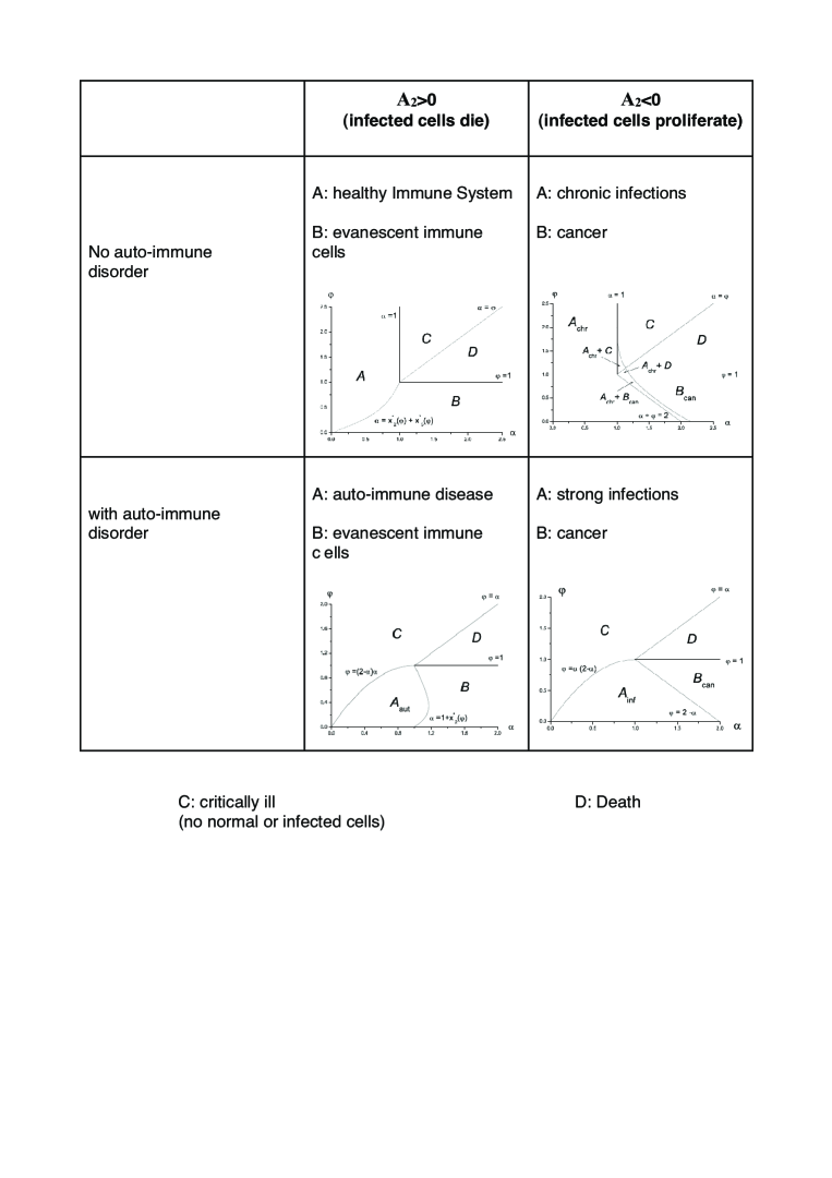
Figure 11: Synthetic table summary of the different states of the organism. $C$ denotes the critically ill state. $D$ represents death.

We have derived a model of immune system homeostasis, describing complex interactions between healthy cells, infected cells, immune system, and pathogens. The model is represented in full generality by a five-dimensional dynamical system, but we have considered here a simplified four dimensional system obtained by assuming symmetric strengths of the responses of the innate and adaptive components of the immune system. The richness of this system provides a classification of a rather diverse set of afflictions typified by important human diseases. Here, we have concentrated our attention on the investigation of the basic topological structure of the dynamical system. Analysing the existence of stationary states and their stability, we have discovered that the model is surprisingly structurally stable when changing two sets of control parameters. We have specifically explored the influence of an auto-immune disorder and of the possibility of infected cells to proliferate. We have thus considered four cases represented schematically in Figure 11:

1. no auto-immune disorder ($a_{13}=a_{31}=a_{14}=a_{41}=0$) and no proliferation of infected cells ($a_{2}>0$)

2. auto-immune disorder ($a_{13}=a_{31}=a_{14}=a_{41}>0$) and no proliferation of infected cells ($a_{2}>0$)

3. no auto-immune disorder ($a_{13}=a_{31}=a_{14}=a_{41}=0$) and proliferation of infected cells ($a_{2}<0$)

4. auto-immune disorder ($a_{13}=a_{31}=a_{14}=a_{41}>0$) and proliferation of infected cells ($a_{2}<0$).

By doing this, we consider the parameters $a_{2}$ and $a_{13},a_{31},a_{14},a_{41}$ as determined exogenously. Their variations which span the four above regions leads to different states, as shown in figure 11. In reality, one would like to have a more complete description in which the dynamics of these parameters is not imposed externally but is endogenized. Our present approach allows us to classify the different states under the condition that the auto-immune propensity and the proliferation tendency of infected cells are kept fixed. Making endogenous the dynamics of these control parameters (which in this way would become more like “order parameters”) may give rise to new phenomena, but this is beyond the first exploratory scope of the present paper.

An example of the possible time evolution of the parameters $a_{13},a_{31},a_{14},a_{41}$ occurs during chronic infections characterized by a strong response of the immune system, which may eventually evolve to some auto-immune disorder due to the strengthening synthesis of antibodies reacting to the membranes of the infected cells deteriorating into attacks of the membrane of normal cells. This phenomenon occurs for instance for hepatic cirrhosis due to hepatitis C virus (HCV), in which cirrhosis is due to the chronic inflammatory response against the liver cells rather than the virus itself.

In each of the four cases, we find four stable stationary states whose boundaries are determined by the values of the system parameters and in particular by the apoptosis rate $\alpha$ and the pathogen flux $\varphi$. The transitions between the states is reminiscent of the phase transitions in statistical systems (Yukalov and Shumovsky, 1990; Sornette, 2006). The occurrence of a given state essentially depends on the balance between the strength of the immune system, characterized by its apoptosis rate, and the external influx of pathogens, which supports the concept that the homeostasis of the organism is governed by a competition between endogenous and exogenous factors. It is important to stress that stable stationary states exist only if the apoptosis in the immune system prevails over the reproduction of immune cells, so that the effective rate $\alpha$ be positive.

This study and the proposed model presented in section 3 has been motivated by the endo-exo hypothesis discussed in section 2. The existence of State A, which describes an organism with a “healthy” immune system, capable of controlling any amount of exogenous pathogen flux, provides a clear embodiment of this concept. The fact that the healthy state A exists only under the influence of a sufficiently large pathogen flux $\varphi$ suggests that health is not the absence of pathogens, but rather a strong ability to find balance by counteracting any pathogen attack. Furthermore, we also find that the critically ill State C can recover to State A by increasing the strength of the immune system (decreasing the apoptosis rate $\alpha$) but evolves to the death State D if an attempt is made of decreasing too much the pathogen flux. This paradoxical behavior illustrates again that pathogens seem, in our system, to be necessary to ensure recovery and health.

We thus propose that a fundamental change in the way we should think about health and illnesses is required. As an example, a concept such as the basic reproductive ratio $R_{0}$, defined as the average number of secondary cases transmitted by a single infected individual that is placed into a fully susceptible population, is useless in our context. Indeed, $R_{0}$ assumes that there is such a thing as a non-infected state. Then, $R_{0}$ quantifies the initial rate of spread of a disease that appears and invades the initially non-infected population. In the standard classification, there will be an epidemic if $R_{0}>1$, while the epidemic dies out before spreading explosively in the population if $R_{0}<1$. In our case, $R_{0}$ would describe the evolution of the populations of different cells in the organism, starting from an initial state in which $x_{2}\ll 1$ (almost complete absence of infected cells), when a burst of pathogens is suddenly introduced. As can be seen from equations (5) or, in reduced form, (13) with (15), when $x_{2}$ is small (very few infected cells), the equation controlling the early dynamics of infected cells is $dx_{2}/dt=-x_{2}\left(\alpha_{2}+a_{23}y+a_{25}x_{5}\right)+a_{51}x_{1}x_{5}$. Since $a_{23}$ and $a_{25}$ are always positive, when $\alpha_{2}>0$, the initial proportional growth rate (the bracket term in factor of $x_{2}$ in the r.h.s.) is always positive, and minus this term is always negative, so that $R_{0}$ is by definition always less than $1$. In the case where $\alpha_{2}<0$ (referred to above as the regime with “proliferation of infected cells), $R_{0}$ can be larger than $1$ if $\alpha_{2}+a_{23}y+a_{25}x_{5}$ is negative. However, this analysis is misleading because it neglects the different channel $a_{51}x_{1}x_{5}$, in the presence of the complex feedback loops described by equations (13) with (15) and the fact that any set of parameters corresponds to a well-defined equilibrium state (except for the case of proliferating infected cells in the absence of auto-immune disorder, in which there is a zone of coexistence of two equilibrium states as shown in figure 7). The argument on the uselessness of the concept of $R_{0}$ in our context can be made clearer by considering an hypothetical pure organism with initial values $x_{2}=y=x_{5}=0$, i.e., made only of normal cells, for which $R_{0}=1-\alpha_{2}$. Hence, the sign of $\alpha_{2}$ determines the initial spread of the disease, according to the standard approach. But, as our analysis has shown, this measure is completely misleading and cannot represent the complex reality of the dynamical evolution of the organism into an homeostatic state characterized by a subtle balance between the immune system response to ever present pathogens and infected cells. Our approach has emphasized that a correct description of the homeostatic equilibrium of an organism is through the determination of the stable fixed points of the system dynamics. Once the organism is in a given stationary state, its dynamics is controlled by the Lyapunov exponents which take automatically into account the different coupling terms between the dynamical variables. By definition of the stability of the fixed points, the Lyapunov exponents are all negative. In contrast, the concept of the basic reproductive ratio implies that it makes sense to imagine the situation of a completely non-infected organism which is suddenly plunged into a situation described by a specific value of the pair $(\alpha,\phi)$ and of the parameters controlling for the existence or absence of an auto-immune disorder and of the proliferation of infected cells. The basic reproductive ratio would then quantify how this hypothetical organism would see its number of infected cells grow initially, to eventually converge to the corresponding equilibrium state associated with these control parameters.

It is possible to generalize the concept of the basic reproductive ratio into the rate of evolution from one state to a neighboring one when the border between two domains of stability is crossed. But this corresponds to a different approach, based on changing the control parameters, in contrast with the initial-value approach implied by the basic reproductive ratio $R_{0}$. Such dynamical evolution is left for another study.

Our results provide insights in so-called regeneration medicine (spontaneous recovery from near extinction, or similarly defined). Actually, our phase diagrams illustrate several cases where regeneration can spontaneously occur. The most obvious one is shown in figure 7 in the coexistence regions for the case of a patient with proliferating ill cells in the absence of auto-immune disorder. In the presence of ubiquitous random perturbations and noise, we predicted that a patient in the critically ill state $C$ or in the cancer state $B_{\rm can}$ can spontaneously recover (partially) to the chronically ill state $A_{\rm chr}$. This regeneration can be viewed as an “emergent” property of the immune system, in the sense that it is a fundamental equilibrium structure derived non-trivially from the basic rules of interactions between the five compartments of the organism. Another paradoxical instance where spontaneous regeneration occurs is shown in figure 1: as discussed in section 4.2, a patient with an evanescent and highly vulnerable immune system may recover to the healthy state $A$ upon an increase of the flux of pathogens, all other things remaining equal! By making endogenous the dynamics of $\alpha$ and $\phi$, no doubt that other paradoxical and surprising regeneration processes will be found. In light of the increasing importance of regenerative medicine and the promise it holds for the future of the critically ill and injured, our model provides an attractive starting point to formulate the different instances of regeneration that can exist.

It goes without saying that, in real life, the parameters of the dynamical system, characterizing any organism, are not necessarily constant, and external conditions are always varying. Therefore, the next step requires us to study the dynamics of the suggested model, including random variations of the pathogen influx and of system parameters. It would, however, be unreasonable to blindly fix the parameters, having so many of them. We plan in our future work to consider the model dynamics specifying the parameters for some particular medical situations.

Appendix A. Lyapunov Stability Analysis

The stability analysis of the considered system of equations is based on the following Lyapunov theorem (see, e.g., Chetaev 1990).

Theorem. Let us consider a system of nonlinear autonomous differential equations

$$\frac{dx_{i}}{dt}=f_{i}(x),\qquad\qquad\qquad\qquad(A.1)$$

where $x\equiv\{x_{i}:\;i=1,2,\ldots,n\}$. Let $x^{*}=\{x_{i}^{*}\}$ be a set of stationary solutions to Eq. (A.1) and the functions $f_{i}(x)$, for all $i=1,2,\ldots,n$, be holomorphic in the vicinity of $x^{*}$. And let $J_{i}(x)$ be the eigenvalues of the Jacobian matrix $[J_{ij}(x)]=[\partial f_{i}/\partial x_{j}]$.

If all Lyapunov exponents $\lambda_{i}\equiv{\rm Re}J_{j}(x^{*})$ are negative, then the solution $x^{*}$ is asymptotically stable, hence, Lyapunov stable. In contrast, if at least one of the Lyapunov exponents $\lambda_{i}$ is positive, then the solution $x^{*}$ is unstable.

In our case, the right-hand sides of Eq. (13), defined in Eqs. (14) to (18), are holomorphic by construction. Thus, the condition for the validity of the Lyapunov theorem is satisfied. We accomplished the stability analysis for each of the four different situations investigated in our paper.

(i) For the case of decaying ill cells without auto-immune disorder, the dynamical system is characterized by the right-hand sides of Eqs. (25) and (26). The equations for the stationary solutions are

$$x_{1}(1-x_{1}-x_{5})=0\;,\qquad x_{2}(1+x_{5}+y)-x_{1}x_{5}=0\;,$$

$$y(x_{2}+x_{5}-\alpha)=0\;,\qquad x_{5}(x_{2}-y-1)+\varphi=0\;.$$

This system of equations has 10 sets of stationary solutions $\{x_{1}^{(k)},x_{2}^{(k)},y^{(k)},x_{5}^{(k)}\}$, with $k=1,\ldots,10$.

Out of these 10 fixed points, only four of them are admissible as possible states of the organism, in the sense that all their normalized cell concentrations are non-negative. The other 6 fixed points are not considered further, as they lie in the non-biological part of the phase diagram $\{x_{1},x_{2},y,x_{5}\}$. The four admissible fixed points are denoted $A$, $B$, $C$, $D$ (see classification of these solutions and their expressions in Sec. 4.2). The corresponding domain of existence of these four different fixed points are presented in Fig. 1.

Then, following closely the Lyapunov theorem, we calculate the Jacobians for each of the four sets $A$, $B$, $C$, $D$ of admissible fixed points and determine the corresponding eigenvalues. We check if the real parts of the eigenvalues are negative. The procedure is straightforward. The analytical expressions for the eigenvalues were obtained by Mathematica. We do not provide here the exact formulas of the eigenvalues because they are extremely cumbersome. Numerical, and when possible, analytical investigations of the real parts of the eigenvalues as functions of parameters $\alpha$ and $\varphi$ have been performed. These investigations led to the determination of the regions of stability (negative values of the real parts of the eigenvalues) for each of the four fixed points according to the phase diagram shown in Fig. 1.

(ii) The case of decaying ill cells with auto-immune disorder is described by the functions (41). The equations for the stationary solutions are

$$x_{1}(1-x_{1}-x_{5}-y)=0\;,\qquad x_{2}(1+x_{5}+y)-x_{1}x_{5}=0\;,$$

$$y(x_{1}+x_{2}+x_{5}-\alpha)=0\;,\qquad x_{5}(x_{2}-y-1)+\varphi=0\;.$$

There are 9 sets of solutions to this system of equations, but only 4 of them are admissible, having all non-negative normalized cell concentrations. These 4 sets of solutions are again denoted as $A$, $B$, $C$, $D$, and are presented in Sec.4.3.

The stability of these four stationary solutions is checked by following the Lyapunov theorem. Our investigations show that all real parts of the eigenvalues of the corresponding Jacobian matrices are negative inside the regions shown in Fig. 5, qualifying the stability of these fixed points $A$, $B$, $C$, $D$ in their respective domains of existence.

(iii) The homeostasis with proliferating ill cells without auto-immune disorder is characterized by the functions given by (52). The stationary solutions are given by the equations

$$x_{1}(1-x_{1}-x_{5})=0\;,\qquad x_{2}(1-x_{5}-y)+x_{1}x_{5}=0\;,$$

$$y(x_{2}+x_{5}-\alpha)=0\;,\qquad x_{5}(x_{2}-y-1)+\varphi=0\;.$$

There are 10 sets of solutions to this system of equations, and again only 4 sets are admissible. These sets of solutions correspond to the states $A$, $B$, $C$, $D$, and are presented in Sec.5.2. The regions of existence of these solutions are shown in Fig. 7. According to the Lyapunov stability analysis, the given states are found to be stable in the corresponding existence regions.

(iv) The case of proliferating ill cells with auto-immune disorder is characterized by the dynamical system with the functions given in (60). The system of equations for the stationary solutions reads as

$$x_{1}(x_{1}+x_{5}+y-1)=0\;,\qquad x_{2}(1-x_{5}-y)+x_{1}x_{5}=0\;,$$

$$y(x_{1}+x_{2}+x_{5}-\alpha)=0\;,\qquad x_{5}(x_{2}-y-1)+\varphi=0\;.$$

There are 9 sets of solutions to this system of equations. And again, only 4 sets of solutions are admissible. These sets of solutions $A$, $B$, $C$, $D$ are described in Sec.5.3. The regions of existence of these solutions are shown in Fig. 9. According to the Lyapunov stability analysis, the given states are stable in the corresponding existence regions.

For each of these cases, we found all stationary solutions and analysed their stability according to the Lyapunov theorem. It turned out that all solutions in the considered cases (Sections 4.2, 4.3, 5.2, and 5.3) are stable in their domains of existence. In addition to the Lyapunov stability analysis, we have checked the stability of the fixed points by intensive direct numerical calculations solving the system (13) for different initial values taken in the vicinity of the stationary points and for different parameters $\alpha$ and $\varphi$. The direct numerical calculations for the whole dynamical system were found to be in complete agreement with the stability analysis based on the Lyapunov theorem.

References

Anderson, P.W., 1972. More is Different, Science 177 (4047), 393-396.

Arneodo, A., Coullet, P., Tresser, C., 1980. Occurrence of strange attractors in three-dimensional Volterra equations. Phys. Lett. A 79, 259-263.

Beisswenger C, Kandler K, Hess C, Garn H, Felgentreff K, Wegmann M, Renz H, Vogelmeier C, Bals R. (2006) Allergic airway inflammation inhibits pulmonary antibacterial host defense, J Immunol. 177, 1833-1837.

Benton, T.G., 2006. Revealing the ghost in the machine: Using spectral analysis to understand the influence of noise on population dynamics. Proc. Natl. Acad. Sci. 103, 18387-18388.

Blaser, MJ. and D. Kirschner, 2007. The equilibria that allow bacterial persistence in human hosts, Nature 449, 843-849.

Bollinger, R.R., A.S. Barbas, E.L. Bush, S.S. Lin and W. Parker, 2007. Biofilms in the large bowel suggest an apparent function of the human vermiform appendix, J. Theor. Biology, in press, doi:10.1016/j.jtbi.2007.08.032

Brown, K.S., Hill, C.C., Calero, G.A., Myers, C.R., Lee, K.H., Sethna, J.P., Cerione, R.A., 2004. The statistical mechanics of complex signaling networks: nerve growth factor signaling. Phys. Biol. 1, 184-195.

Brown, K.S., Sethna, J.P., 2003. Statistical mechanics approaches to models with many poorly known parameters. Phys. Rev. E 68, 021904-9.

Canuyt, G., 1932. Fixation Abscess, The Journal of Laryngology & Otology 47, 235-242.

Chetaev N.G., 1990. Stability of Motion. Nauka, Moscow.

Ginoux, J.M., Rossetto, B., Jamet, J.L., 2005. Chaos in a three-dimensional Volterra-Gause model of predator-prey type. Int. J. Bifurc. Chaos 15, 1689-1708.

Hofbauer, J., Sigmund, K., 2002. Evolutionary Games and Population Dynamics. Cambridge University, Cambridge.

Hsu, S.-B. T.-W. Hwang, Y. Kuang, 2001. Rich dynamics of a ratio-dependent one-prey two-predators model, J. Math. Biol. 43, 377-396.

Krammer, P.H., 2000. CD95’s deadly mission in the immune system. Nature 407, 789-795.

Louzoun, Y., 2007. The evolution of mathematical immunology, Immunological Reviews, 216, 9-20.

Marsland, B.J,. Nembrini, C., Schmitz, N., Abel, B., Krautwald, S., Bachmann, and M.F., Kopf, M., 2005a. Innate signals compensate for the absence of PKC-theta during in vivo CD8(+) T cell effector and memory responses, Proc Natl Acad Sci U S A. 102(40), 14374-14379.

Marsland, B.J., Battig, P., Bauer, M., Ruedl, C., Lassing, U., Beerli, R.R., Dietmeier, K., Ivanova, L., Pfister, T., Vogt, L., Nakano, H., Nembrini, C., Saudan, P., Kopf, M., and Bachmann, M.F. 2005b. CCL19 and CCL21 induce a potent proinflammatory differentiation program in licensed dendritic cells. Immunity 22(4), 493-505.

Matzinger, P., 2002. The Danger Model: A renewed sense of self, Science 296, 301-305.

Mazmanian, S.K., Liu, C.H., Tzianabos, A.O., Kasper, D.L., 2005. An immunomodulatory molecule of symbiotic bacteria directs maturation of the host immune system. Cell 122, 107-118.

McFall-Ngai, M., 2007. Care for the community, Nature 445, 153-153.

Nelson, P.W., Perelson, A.S., 2002. Mathematical analysis of delay differential equation models of HIV-1 infection. Math. Biosciences 179, 73-94.

Nowak, M.A., 2006. Evolutionary Dynamics: Exploring the Equations of Life, Belknap Press.

Palmer, C., Bick, E.M., DiGiulio, D.B., Relman, D.A., Brown, P.O., 2007. Development of the human infant intestinal microbiota. Plos Biology 5, 1556-1573.

Perelson, A.S., 2002. Modelling viral and immune system dynamics. Nature 2, 28-36.

Perelson, A.S., Weisbuch, G., 1997. Immunology for physicists. Rev. Mod. Phys. 69, 1219-1268.

Reuman, D.C., Desharnais, R.A., Constantino, R.F., Ahmad, O.S., Cohen, J.E., 2006. Power spectra reveal the influence of stochasticity on nonlinear population dynamics. Proc. Natl. Acad. Sci. 103, 18860-18865.

Schaub, B., R. Lauener, and E. von Mutius, 2006. The many faces of the hygiene hypothesis J. Allergy Clin. Immunol. 117(5), 969-977.

Scott, A., 2005. Encyclopedia of Nonlinear Science. Routledge, New York.

Sornette, D., 2005. Endogenous versus exogenous origins of crises. In: Extreme Events in Nature and Society, Albeverio, S., Jentsch, V., Kantz, H. eds., Springer, Heidelberg.

Sornette, D., 2006. Critical Phenomena in Natural Sciences. Springer, Berlin.

Sornette, D., Deschatres, F., Gilbert, T., Ageon, Y., 2004. Endogenous versus exogenous shocks in complex networks: an empirical test using book sale ranking. Phys. Rev. Lett. 93, 228701.

Sornette, D., Helmstetter, A., 2003. Endogenous versus exogenous shocks in systems with memory. Physica A 318, 577-591.

Sornette, D., Malevergne, Y., Muzy, J.F., 2003. Tail risk: what causes crashes. Risk 16, 67-71.

Strachan, D.P. 1989. Hay fever, hygiene, and household size, British Medical J. 299, 1259-1260.

Xiang, Z. and X. Song, 2006. Extinction and permanence of a two-prey two-predator system with impulsive on the predator, Chaos Solit. Fract. 29, 1121-1136.

Young, L.R., 1999. Artificial gravity considerations for a Mars Exploration Mission, Ann. NY Acad. Sci. 871, 367-378.

Yukalov V.I., Shumovsky, A.S., 1990. Lectures on Phase Transitions. World Scientific, Singapore.

Figure 1: Phase portrait in the plane $\alpha,\varphi$ showing the stability regions for four stationary states (A, B,C, and D), when the immune system does not attack healthy cells (no auto-immune disorder).

                 

                 

Figure 2: State $A$: Stationary solutions for the normalized cell numbers and pathogens as functions of the apoptosis rate $\alpha$ for different pathogen fluxes $\varphi=0.5$ (solid line), $\varphi=1$ (dashed line), and $\varphi=5$ (dotted line) in the case of no auto-immune disorder.

Figure 3: State $B$: Stationary solutions (31) for the normalized cell numbers and pathogens as functions of $\varphi$ in the absence of auto-immune disorder. $x_{1}(\varphi)$ (solid line), $x_{2}(\varphi)$ (dashed line), and $x_{5}(\varphi)$ (dotted line).

Figure 4: State $C$: Stationary solution (36) for the immune normalized cell numbers $y^{*}(\alpha,\varphi)$ as a function of $\alpha$ for different $\varphi=1.5$ (solid line), $\varphi=3$ (dashed line), and $\varphi=5$ (dotted line) in the absence of auto-immune disorder.

Figure 5: Phase portrait for the stability regions of the stationary states, in the case with auto-immune disorder.

                 

                 

Figure 6: State $A_{\rm aut}$: Stationary solutions for the normalized cell numbers and pathogens as functions of the apoptosis rate $\alpha$ for different pathogen fluxes $\varphi=0.2$ (solid line), $\varphi=0.6$ (dashed line), and $\varphi=0.9$ (dotted line) in the case with auto-immune disorder. The solutions are shown in the region of their existence.

Figure 7: Phase portrait on the plane $\alpha,\varphi$ for the case of proliferating ill cells in the absence of auto-immune disorder

                 

                 

Figure 8: State $A_{\rm chr}$: Stationary solutions for the normalized cell numbers and pathogens as functions of the apoptosis rate $\alpha$ for several pathogen fluxes $\varphi=0.2$ (solid line), $\varphi=0.9$ (dashed line), and $\varphi=2$ (dotted line), in the case 5.2 of proliferating ill cells, in the absence of auto-immune disorder.

Figure 9: Phase portrait on the $\alpha-\varphi$ plane for the stability regions of the stationary solutions in the case of proliferating ill cells and of auto-immune disorder.

                 

Figure 10: State $A_{\rm inf}$ of Subsection 5.3, defined by Eqs. (61). The nontrivial solutions for the normalized cell numbers and pathogens as functions of $\alpha$ for different $\varphi=0.2$ (solid line), $\varphi=0.6$ (dashed line), and $\varphi=0.9$ (dotted line), in the case of proliferating ill cells in the presence of auto-immune disorder.