Localizing coalescing massive black hole binaries with gravitational waves
Abstract
Massive black hole binary coalescences are prime targets for space-based gravitational wave (GW) observatories such as LISA. GW measurements can localize the position of a coalescing binary on the sky to an ellipse with a major axis of a few tens of arcminutes to a few degrees, depending on source redshift, and a minor axis which is times smaller. Neglecting weak gravitational lensing, the GWs would also determine the source’s luminosity distance to better than percent accuracy for close sources, degrading to several percent for more distant sources. Weak lensing cannot, in fact, be neglected and is expected to limit the accuracy with which distances can be fixed to errors no less than a few percent. Assuming a well-measured cosmology, the source’s redshift could be inferred with similar accuracy. GWs alone can thus pinpoint a binary to a three-dimensional “pixel” which can help guide searches for the hosts of these events. We examine the time evolution of this pixel, studying it at merger and at several intervals before merger. One day before merger, the major axis of the error ellipse is typically larger than its final value by a factor of . The minor axis is larger by a factor of , and, neglecting lensing, the error in the luminosity distance is larger by a factor of . This large change over a short period of time is due to spin-induced precession, which is strongest in the final days before merger. The evolution is slower as we go back further in time. For , we find that GWs will localize a coalescing binary to within as early as a month prior to merger and determine distance (and hence redshift) to several percent.
1 Introduction
Among the most important sources of gravitational waves (GWs) in the low-frequency band of space-based detectors are the coalescences of massive black hole binaries (MBHBs). Binaries containing black holes with masses in the range are predicted to form through the hierarchical growth of structure as dark matter halos (and the galaxies they host) repeatedly merge; see, for example, Sesana et al. (2007) and Micic et al. (2007) for recent discussion. The Laser Interferometer Space Antenna (LISA) is being designed to have a sensitivity that would allow detailed measurement of the waves from these binaries. “Intrinsic” parameters — the masses and spins of the black holes which compose the binary — should be determined with very high accuracy, with relative errors typically to , depending on system mass and redshift; see Lang & Hughes (2006, hereafter Paper I) for recent discussion. By measuring an ensemble of coalescences over a range of redshifts, MBHB GWs may serve as a kind of structure tracer, tracking the growth and spin evolution of black holes over cosmic time.
“Extrinsic” system parameters, describing a binary’s location and orientation relative to the detector, are also determined by measuring its GWs. In Paper I, we showed that a binary’s position on the sky can be localized at to an ellipse with a major axis of a few tens of arcminutes and a minor axis a factor of smaller. At higher redshift (), these values degrade by a factor of a few, reaching a few degrees in the long direction and tens of arcminutes to a degree or two in the short one. We also found that, neglecting errors due to weak gravitational lensing, a source’s luminosity distance typically can be determined to better at low redshift (), degrading to several percent at higher redshift ().
The intrinsic ability of GWs to determine the distance to a coalescing binary is phenomenal. Coalescing MBHB systems constitute exquisitely well calibrated distance measures, with the calibration provided by general relativity. Unfortunately, this percent-level or better accuracy could only be achieved if we measured MBHB coalescences in an empty universe. In our universe, weak lensing will magnify or demagnify the GWs, and we will infer a luminosity distance smaller (for magnification) or larger (for demagnification) than the true value. This phenomenon affects all high-redshift standard candles. Its impact on Type Ia supernovae in particular has been discussed in detail (Frieman, 1997; Holz & Wald, 1998; Holz, 1998). It will not be possible to correct for this effect (Dalal et al., 2003) since much of the lensing “noise” arises from structure on subarcminute scales that is not probed by shear maps (which map the distribution of matter on scales greater than or so). Since we will not know the extent of the magnification when we measure MBHB waves, we must simply accept the fact that lensing introduces a dispersion of several percent in determining the distance to these GW events (see, e.g., Wang et al. [2002] to compute this dispersion as a function of redshift). When we quote distance measurement errors, we will typically quote only the intrinsic GW measurement error, neglecting lensing’s impact. When the intrinsic GW distance error is , lensing will blur it to the several percent level.
Note that a source’s redshift cannot be directly determined using only GWs. Gravitational wave measurements infer system parameters through their impact on certain dynamical timescales, such as orbital frequencies and the rate at which these frequencies evolve. Since these time scales all suffer cosmological redshift, is degenerate with other parameters. For example, any mass parameter is actually measured as . However, if the binary’s luminosity distance is determined, its redshift can then be inferred by assuming a cosmography. For most binaries, the redshift can be determined to several percent (with an error budget dominated by gravitational lensing111At redshifts , the error is actually dominated by peculiar velocity effects (Kocsis et al., 2006); however, the event rate is probably negligible at such low redshifts. As such, we will focus on gravitational lensing as the main source of systematic redshift error.). We thus expect that GW measurements will locate a binary to within a three-dimensional “GW pixel” which at has a cross-sectional area of to and a depth several percent.
It is anticipated that there will be great interest in searching the GW pixel for electromagnetic (e.g., optical, X-ray, radio) counterparts to MBHB GW events. Finding such a counterpart would be much easier if galactic activity were catalyzed in association with the coalescence (Kocsis et al., 2006). The nature of that activity is likely to depend rather strongly on the mass of the coalescing system (Dotti et al., 2006). For example, Armitage & Natarajan (2002) predict strong outflows and galactic activity prior to the final black hole merger as the smaller member of the binary drives gas onto the larger member, consistent with the high-mass () predictions of Dotti et al. (2006). Milosavljević & Phinney (2005) describe an X-ray afterglow that would ignite after gas refills the volume that is swept clean by the coalescing binary; Dotti et al. predict this outcome for smaller systems (). Recent work by Bode & Phinney (2007) suggests that the final burst of radiation from a coalescing binary (which can convert of the system’s mass to GWs very suddenly) may excite radial waves, and consequently electromagnetic variability, in an accretion disk due to the quick change in the disk’s Keplerian potential. Such a signature may be essentially mass independent. On the other hand, the coalescence may be electromagnetically quiet, in which case we face the potentially daunting task of searching the three-dimensional pixel for galaxies with morphology consistent with a (relatively) recent merger, or that have a central velocity dispersion consistent with the inferred final black hole mass (assuming that the relation [Ferrarese & Merritt 2000; Gebhardt et al. 2000] holds at the redshift of these sources, and so soon after merger).
If the host galaxy or some other counterpart can be identified, we could then contemplate combining GW information with electromagnetic data. For instance, combining LISA mass measurements with the luminosity of the counterpart may allow us to directly measure the Eddington ratio (Kocsis et al., 2006). Identifying a counterpart would also allow us to more accurately characterize the system. For example, much of the intrinsic luminosity distance error is due to correlations between distance and sky position. Finding an electromagnetic counterpart essentially determines a binary’s position precisely, breaking those correlations. Previous studies have found that intrinsic distance error can be reduced by almost an order of magnitude if the position is known (Hughes, 2002; Holz & Hughes, 2005). (Lensing errors still dominate in such a case, so that the distance remains determined only at the few percent level.) A counterpart may also make it possible to simultaneously determine a source’s luminosity distance and redshift. Such a “standard siren” (the GW analog of a standard candle) would very usefully complement other high-redshift standard candles (Holz & Hughes, 2005), such as Type Ia supernovae (Phillips, 1993; Riess et al., 1995; Wang et al., 2003). A direct measurement of redshift will also break the mass-redshift degeneracy more accurately than can be done with just the luminosity distance and some assumed cosmological parameters. Breaking this degeneracy is critical when studying the growth of black holes with cosmic time (Hughes, 2002).
Many analyses (Cutler, 1998; Hughes, 2002; Vecchio, 2004; Berti et al., 2005; Holz & Hughes, 2005) have quantified how well LISA can determine MBHB parameters, including sky position and distance, using maximum likelihood Fisher matrix estimation. Our results from Paper I, given earlier, include the effects of “spin-induced precession” — precession of both the orbital plane and the individual spins of the black holes due to post-Newtonian spin-interaction effects. A significant result from that analysis is that spin-induced precession improves sky position accuracy by about half an order of magnitude in each direction versus previous analyses. This result can be partially understood as due to the breaking of a degeneracy between position and orientation angles: thanks to precession, the binary’s orientation evolves with time and can be untangled from sky position. This effect was already known due to pioneering work by Vecchio (2004); by taking the analysis to higher order and considering a broader range of sources, we were able to show that this improvement held for essentially all astrophysically interesting MBHB sources.
The purpose of this paper is to examine the localization of MBHB systems more thoroughly, in particular how the GW pixel evolves as the final merger is approached. Paper I only presented results for measurements that proceed all the way to merger. It will clearly be of some interest to monitor potential hosts for the binary event some time before the merger happens; if nothing else, telescopes will need prior warning to schedule observing campaigns. Understanding the rate at which localization evolves can also have an important impact on the design of the LISA mission, clarifying how often it will be necessary to downlink data about MBHB systems in order to effectively guide surveys.
Our main goal is to understand for what range of masses and redshifts prior localization of a binary using GWs will be possible. A previous analysis by Kocsis et al. (2007b; hereafter K07) also examined this problem in great detail, but without including the impact of spin-induced precession. One of our goals is to see to what extent precession physics changes the conclusions of K07. We find that precession has a fairly small impact on the time evolution of the GW pixel except in the last few days before the final merger, at which point its impact can be tremendous. Precession typically changes the area of the sky position error ellipse by a factor of (up to in extreme cases) in just the final day. This is in accord with the predictions of K07 (and even earlier predictions by N. Cornish 2005, unpublished).
The structure of this paper is as follows. First, in § 2, we briefly review the basics of the MBHB gravitational waveform and the parameter estimation formalism that we use; this section is essentially a synopsis of relevant material from Paper I. Section 2.1 reviews the form of the GWs that we use in our analysis, while § 2.2 describes how those waves are measured by the LISA constellation. We describe the measurement formalism we use in § 2.3. In § 2.4, we summarize our results from Paper I regarding the final localization accuracy that LISA can expect to achieve.
We turn to a detailed discussion of the time evolution of the GW pixel in § 3. We begin by summarizing the key ideas behind the “harmonic mode decomposition” of K07 in § 3.1. This technique cleverly allows calculation of the GW pixel and its time evolution with much less computational effort than our method (albeit without including the impact of spin precession). Unfortunately, we have discovered that some of the approximations used by K07 introduce a systematic underestimate of the final sky position error by a factor of or more in angle; the approximations are much more reliable a week or more prior to the black holes’ final merger. Modulo this underestimate, the K07 results agree well with a version of our code which does not include spin precession (particularly a week or more in advance of merger, when their underestimate is not severe). K07 thus serves as a useful point of comparison to establish the impact of precession on source localization.
Section 3.2 is dedicated to our results, including comparison to K07 when appropriate. We find that all relevant parameter errors decrease slowly with time until the last day before merger, when they drop more dramatically. This sudden drop is not found in K07, nor is it present in a variant of our analysis that ignores spin precession. It clearly can be attributed to the impact of precession on the waveform. Before this last day, the major axis is times, the minor axis times, and the intrinsic error in the luminosity distance times bigger than at merger for most binaries (i.e., all except the highest masses). Going back to one week (one month) before merger, these numbers change to () for the major axis, () for the minor axis, and () for the error in the luminosity distance. As a result, for , most binaries can be located within a few square degrees a week before merger and a month before merger. The intrinsic distance errors are also small enough this early that remains dominated by gravitational lensing errors of several percent. Advanced localization of MBHB coalescences thus seems plausible for these binaries; the situation is less promising for sources at higher redshift.
As a corollary to our study of the time evolution, we also examine the sky position dependence of errors (§ 3.3). The errors depend strongly on the polar angle with respect to the ecliptic, increasing in the ecliptic plane to as much as over the median for the major axis, over the median for the minor axis, and over the median for errors in the luminosity distance. The errors have a much weaker dependence on the azimuthal angle. When we convert to Galactic coordinates, we find that the best localization regions appear to lie fairly far out of the Galactic plane, offering hope that searches for counterparts will not be too badly impacted by foreground contamination.
We conclude this paper in § 4. Besides summarizing our results, we discuss shortcomings of this analysis and future work which could help to better understand how well GWs can localize MBHB sources.
Throughout the paper we set ; a convenient conversion factor in this system is s. When discussing results, we always quote masses as they would be measured in the rest frame of the source. These masses must be multiplied by a factor of when used in any of the equations describing the system’s dynamics or its GWs (particularly the equations of § 2). We convert between distance and redshift using a spatially flat cosmology with (and hence ) and Hubble constant .
2 Determining the sky position and distance accuracy of LISA
In this section, we present necessary background. We begin by summarizing the inspiral GW signal and its measurement by LISA. We then describe the parameter estimation formalism that we use in our code. More details on these topics can be found in Paper I and references therein. Finally, we present a synopsis of the results from Paper I, summarizing the final sky position and distance accuracy that LISA can expect to achieve. Detailed discussion of how this accuracy evolves as a function of time is deferred to § 3.
2.1 MBHB gravitational waves
As is by now traditional, we break the GWs generated by a coalescing binary black hole system into three more or less distinct epochs: (1) a slowly evolving inspiral, in which the black holes gradually spiral toward each other as the orbit decays due to GW emission; (2) a loud merger, in which the black holes come together and form a single body; and (3) a ringdown, in which the merged remnant of the binary settles down to its final state. Our analysis focuses on the inspiral, the most long-lived epoch of coalescence and the epoch in which spin precession plays a major dynamical role. The inspiral’s duration means that LISA’s position and orientation changes considerably during the measurement; this, plus the impact of precession, is largely responsible for pinning down the sky position of coalescing sources.
The inspiral GW signal is modeled using the post-Newtonian (PN) formalism (Blanchet, 2006; Blanchet et al., 1995; Will & Wiseman, 1996). More specifically, we use the “restricted” PN approximation. The waveform can be written schematically as (Cutler & Flanagan, 1994)
| (1) |
where labels PN order, is a harmonic index, and is the orbital phase. In the restricted PN case, we discard all amplitudes except the strongest Newtonian quadrupole, . The phase, however, is computed to a desired PN order (here the second one, or 2PN). It has been recognized for some time that important additional information is carried by subleading harmonics (e.g., Hellings & Moore 2003). Recent work (Arun et al., 2007; Trias & Sintes, 2008) has confirmed that sky position and distance are more sharply constrained when these terms are included in the wave model (although there still appears to be some disagreement among different groups as to the extent of the improvement). We plan to include these terms in future work, examining how higher harmonics and precession combine to localize MBHB systems.
Spin-induced precession arises from geodetic and gravitomagnetic influences on the angular momentum vectors present in the binary. Averaged over an orbit, the leading-order spin precession equations are (Apostolatos et al., 1994; Kidder, 1995)
| (2) | |||||
| (3) |
where and are the masses of holes 1 and 2, is the total mass, is the reduced mass, is the normal to the orbital plane, and are the spins of the holes, and is their orbital separation in harmonic coordinates. Since total angular momentum is conserved on short timescales (ignoring the inspiral), the orbital angular momentum precesses to compensate. These precessions drive several modifications to the orbital phase. One correction is due to spin-orbit and spin-spin terms in the post-Newtonian expression for orbital frequency: Precession makes these terms time dependent, adding a new modulation to the GW phase. Another correction arises from the changing orientation of the orbital plane (Apostolatos et al., 1994).
The waveform is described as two polarizations propagating in the direction, where gives the direction to the binary on the sky:
| (4) | |||||
| (5) |
where is the frequency of the waves, is the luminosity distance, is the wave phase (twice the orbital phase in the quadrupole approximation), and is the precessional correction to the orbital phase due to the changing orientation of the orbital plane. The “chirp mass” , which controls the frequency evolution, or chirp, of the signal, is given by . Note that the relative weight of the polarizations is determined by the binary’s inclination to the line of sight , where .
2.2 MBHB gravitational waves as measured by LISA
The baseline LISA mission consists of three spacecraft arranged in an equilateral triangle with arms of length km. The center of this constellation orbits the Sun behind the earth, with the triangle oriented at to the ecliptic. The individual spacecraft thus orbit in different planes, causing the triangle to “roll” about itself in its orbit. To model LISA’s response to a signal, we use the long wavelength () approximation introduced by Cutler (1998). The three arms of the triangle act as a pair of two-arm detectors; the signals from the three arms are combined in such a way that the noise spectrum in each “synthesized” detector is independent of the other. Each detector measures both GW polarizations, weighted by antenna response functions and , where labels the synthesized detector. These functions depend on the source’s sky position as measured in the detector frame. Because of the constellation’s rolling orbital motion, these functions are time dependent. The motion around the Sun also causes a Doppler shift in the signal’s frequency. This time dependence allows the sky position of the source to be measured.
An additional time dependence is produced by the precession of the binary’s orbital plane. We saw above that the polarizations strongly depend on the binary’s inclination to the line of sight (via ). The antenna pattern functions also depend on the component of that is perpendicular to the line of sight. Since precession changes the direction of the orbital plane, the measured polarizations would vary in time even if the detector were static. The timescale of these precessions is much shorter than the LISA orbital timescale of 1 yr, so they provide a great deal of additional information about sky position.
We perform the parameter estimation analysis in the frequency domain, so we Fourier transform the signal using the stationary phase approximation. The final measured waveform is given by
| (6) |
where is the “polarization amplitude,” is the “polarization phase,” and is the Doppler phase. The first two encode modulations due to the relative polarization weightings and antenna pattern functions; the latter is due to the Doppler shift in the GW frequency. Full expressions for these functions can be found in Paper I. To second post-Newtonian order, the phase is given by (Poisson & Will, 1995)
| (7) | |||||
where , is the “merger time” (the time at which formally diverges in the post-Newtonian framework), is the phase at , and and are “spin-orbit” and “spin-spin” parameters, respectively, encoding the manner in which interactions between the spins and the orbits impact the phase. See Paper I for precise definitions. For our purposes, the most important property of and is that they oscillate due to precession, modulating the phase . Note that waveform (6) depends on 15 parameters: 2 masses, 6 initial spin components, 1 distance, 2 sky angles, 2 initial orbital plane angles, , and .
The end of inspiral/beginning of merger is a somewhat ad hoc and fuzzy boundary. Indeed, recent numerical computations have shown that the GWs produced by a binary that coalesces into a single body do not show any particular special feature as the black holes come together, instead smoothly chirping through this transition (Buonanno et al., 2007; Pan et al., 2008). Since we are not including numerical merger waves in our analysis, we require some point to terminate our post-Newtonian expansion. Most studies show that the inspiral comes to an end when the separation of the bodies in harmonic coordinates is roughly ; at this point, the system’s GW frequency is approximately given by
| (8) |
where is the Keplerian orbital angular frequency. (The factor converts from angular frequency to frequency; the additional factor of accounts for the quadrupolar nature of gravitational waves.) We use equation (8) throughout our analysis to terminate the inspiral.
2.3 Summary of parameter measurement formalism
To estimate how well LISA will be able to measure MBHB parameters, we use the maximum likelihood formalism developed by Finn (1992). The GW signal described above is corrupted by noise to produce a measured signal . We assume the noise is zero mean, wide-sense stationary, Gaussian, and uncorrelated between the two detectors (). It can be characterized by its (one sided) power spectral density (PSD) , which is described in detail in § IIIB of Paper I. The PSD includes instrumental noise intrinsic to the detector, based on the model described by Larson et al. (2000) and implemented on the World Wide Web222See http://www.srl.caltech.edu/~shane/sensitivity/., with important numerical factors described in § IIC of Berti et al. (2005). It also includes astrophysical noise arising from a confused background of Galactic (Nelemans et al., 2001) and extragalactic (Farmer & Phinney, 2003) white dwarf binaries. With the noise PSD, we can define the inner product between two signals and as
| (9) |
We write a GW as , where the components of the vector represent the 15 parameters describing MBHB waves. We assume that a detection has occurred — that a signal with particular parameters is present in the data — and that maximum likelihood (ML) estimates (Cutler & Flanagan, 1994) of these parameters have been found. The signal-to-noise ratio (S/N) is then given by
| (10) |
Our ultimate goal is to understand the errors in the ML parameters. To do so, we examine the probability that the GW parameters are given by , expanded around the ML estimate (Cutler & Flanagan, 1994; Poisson & Will, 1995):
| (11) |
where and
| (12) |
evaluated at , is known as the Fisher matrix. This expression holds for large values of the S/N and is known as the Gaussian approximation. For the two-detector case, we can exploit the independence of the noises to write the total Fisher matrix as the sum of the individual Fisher matrices. If we define the covariance matrix , we can then estimate the measurement error in some parameter ,
| (13) |
as well as the correlation between two parameters,
| (14) |
We are particularly interested in the sky position, which we parameterize by the coordinates (, ).333The bar over the angles conforms to the notation in Paper I for quantities measured in the solar system barycenter frame, as opposed to those measured in the time-varying detector frame. We want to convert from errors in these two parameters to an error ellipse on the sky. To do so, we first perform a change of coordinates from to . For small deviations from the ML estimate, we have . Next, we recognize that due to the geometric properties of the sphere, the same corresponds to a different “proper” angle depending on the value of : . With these modifications, equation (11) becomes
| (15) |
Here denotes the proper errors accounting for the metric of the sphere, and represents the equivalent Fisher matrix with all conversion factors absorbed inside:
| (16) | ||||
| (17) | ||||
| (18) |
and so on for the rest of the elements. The inverse of this matrix is the proper covariance matrix, . Consider now just the subspace of the covariance matrix containing the sky position variables. Let the eigenvalues of this subspace be . If we define the error ellipse such that the probability that the source lies outside of it is (corresponding to a confidence interval), then the major and minor axes are given by and , respectively. Expressed in terms of the original covariance matrix, these are
| (19) |
Many previous analyses have reported the ellipse’s area or , the side of a square of equivalent area, as the sky position error (Cutler, 1998; Vecchio, 2004; Berti et al., 2005; Holz & Hughes, 2005). Information about the ellipse’s shape, crucial input to coordinating GW observations with telescopes, is not included in such a measure. By examining both and , this information is restored.
In an empty universe, the third dimension of our pixel would be determined from the luminosity distance error, . As already discussed, this quantity is often so small that weak gravitational lensing is expected to dominate the distance error budget. We thus expect
| (20) |
where the lensing dispersion is described in, for example, Wang et al. (2002). If cosmological parameter errors can be neglected, then one typically finds that the redshift error is about equal to the distance error (Hughes, 2002): , independent of redshift.
2.4 Final position and distance accuracy
We conclude this section by reviewing the final accuracy with which MBHB sky position and distance can be determined with GWs. In Paper I, we described the code which implements the measurement formalism described in §§ 2.1 – 2.3 above. This formalism is coupled to a Monte Carlo engine: We specify the rest frame masses and redshift and then randomly choose the sky position, initial angular momentum and spin directions, and spin magnitudes for each binary. We also uniformly distribute the time parameter of each binary over the assumed duration of the LISA mission (which we take to be 3 yr). Some binaries are therefore already “on” when the mission begins, and as such may radiate in band for less time than other binaries which enter the band later. The random distribution of merger times also means that the relative azimuth between a binary’s sky position and LISA’s orbital position at merger, , is itself randomly distributed, even if we choose to focus on a particular . We discuss the implications of this in more detail in § 3.3. Computing the errors for a large number of binaries ( for each mass and redshift set, unless otherwise stated) allows us to make statements about the distribution of parameter errors for different mass and redshift combinations.
Table 1 summarizes the final accuracy of MBHB sky position and distance measurements. Here we show the median measurement accuracy from many Monte Carlo surveys. Several trends are particularly noteworthy. At all redshifts, the accuracy is worst for the largest masses. This is because the most massive systems are in band for the least amount of time: The frequency at which inspiral ends is inversely proportional to mass (see eq. [8]), and more massive systems move more rapidly from low frequency to high frequency. The short time these systems spend in band means that LISA measures a relatively small number of modulations (whether induced by the constellation’s orbit or by spin precession). Second, note that the results for tend to be less accurate than results with similar total mass but for which . The cause of this phenomenon lies in precession equations (2) and (3): When , the two spins precess at different rates, imposing richer modulations on the measured GWs. Since is a rather artificial limit, we expect that the more accurate results for nonunity mass ratio will be the rule.
| 1 | 27.3 | 13.3 | 0.0729 | 0.00398 | ||
| 16.9 | 7.33 | 0.0233 | 0.00240 | |||
| 23.3 | 11.8 | 0.0556 | 0.00357 | |||
| 27.2 | 6.62 | 0.0235 | 0.00320 | |||
| 31.3 | 13.2 | 0.0705 | 0.00393 | |||
| 40.2 | 21.9 | 0.176 | 0.00560 | |||
| 34.1 | 9.20 | 0.0445 | 0.00376 | |||
| 32.3 | 14.7 | 0.0839 | 0.00419 | |||
| 43.3 | 22.3 | 0.193 | 0.00689 | |||
| 37.6 | 12.2 | 0.0670 | 0.00457 | |||
| 42.1 | 19.0 | 0.142 | 0.00610 | |||
| 81.3 | 38.6 | 0.680 | 0.0250 | |||
| 3 | 81.0 | 40.8 | 0.665 | 0.0123 | ||
| 92.5 | 39.5 | 0.656 | 0.0126 | |||
| 142 | 75.7 | 2.15 | 0.0201 | |||
| 141 | 36.6 | 0.739 | 0.0155 | |||
| 129 | 56.7 | 1.25 | 0.0161 | |||
| 158 | 84.3 | 2.64 | 0.0237 | |||
| 132 | 40.3 | 0.751 | 0.0153 | |||
| 142 | 64.6 | 1.65 | 0.0193 | |||
| 224 | 111 | 5.08 | 0.0422 | |||
| 206 | 78.5 | 2.74 | 0.0293 | |||
| 297 | 152 | 9.40 | 0.0805 | |||
| 2000 | 583 | 256 | 2.41 | |||
| 5 | 169 | 85.7 | 2.93 | 0.0260 | ||
| 217 | 95.8 | 3.73 | 0.0284 | |||
| 295 | 161 | 9.29 | 0.0409 | |||
| 248 | 66.8 | 2.35 | 0.0273 | |||
| 233 | 101 | 3.96 | 0.0294 | |||
| 315 | 162 | 10.2 | 0.0501 | |||
| 265 | 86.4 | 3.27 | 0.0318 | |||
| 304 | 139 | 7.52 | 0.0436 | |||
| 538 | 260 | 29.5 | 0.140 | |||
| 577 | 290 | 31.9 | 0.124 | |||
| 1720 | 621 | 234 | 1.24 | |||
| 180000 | 29600 | 377 |
Independent of these trends, an important result is that MBHB systems are pinned down on the sky fairly accurately at . Modulo the higher mass binaries, the median major axis of the sky position error ellipse is typically about , and the median minor axis is about , with a total ellipse area considerably smaller than (ranging from about 0.02 to 0.2 ). Sources at are located accurately enough that one can comfortably contemplate searching the GW error ellipse for MBHB counterparts with future survey instruments, such as the Large Synoptic Survey Telescope (LSST; Tyson et al. 2002).
At higher redshift, positional accuracy degrades. This is due to the weakening of the signal with distance and to the redshifting of the waves’ spectrum, so that the signal tends to spend less time in band. At , the major axis of the error ellipse is across, and the minor axis is . The total area of this ellipse is . At , this degrades further to for the major axis, for the minor axis, and for the total area. These degraded accuracies are still sufficiently well determined that telescopic searches for MBHB counterparts have a good chance to be fruitful (although not nearly as simple as they would be at ).
In all cases, the GW distance determination is extremely accurate: For all but the highest masses, at , at , and at . Distance is determined so precisely that these errors are in fact irrelevant — weak gravitational lensing will dominate the distance error budget for all but the most massive MBHB events.
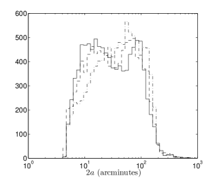
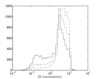
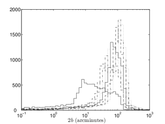
Although the median values reported in Table 1 indicate the typical sky position accuracies we expect, it should be emphasized that they are taken from broad distributions. Figure 1 presents the distributions we computed for binaries at with masses and . Note that the major axis distribution (left) is rather flat when compared to the minor axis distribution (right). It lacks a single well-defined peak; in fact, it is actually bimodal for , with one peak near and another closer to . We find that this behavior holds over all mass and redshift cases of interest, with only slight variations. At smaller masses, the distribution is broader than the cases pictured, without strong bimodality; for larger masses, the distribution is somewhat narrower and tends to develop two very distinct peaks. Higher mass ratios tend to accentuate the peaks. These results hold for higher redshift, except that transitions between various behaviors occur at smaller total mass [in keeping with the fact that it is not mass but times the mass that determines dynamical behavior].
The minor axis distribution exhibits a rather long tail to very small values, especially when the mass ratio is large. For , the distribution peaks near a minor axis , but extends from roughly to about . As the mass ratio approaches 1, the peak moves to slightly larger values (slightly more than for ; roughly for ), and the tail becomes less populated (although the distributions span roughly the same extent as when ). We find that this tail exists for all interesting mass and redshift combinations, with the same strong dependence on mass ratio as shown in Figure 1.
Finally, it is worth emphasizing that spin-induced precession has a significant effect on the accuracy which we report here. In Paper I, we compared these results to those obtained with a code which does not include precession physics. Position and distance accuracy are determined only by the detector’s motion in this case. We found that precession effects reduce the major axis of the sky position error ellipse by a factor of and the minor axis by a factor of . The distance error is likewise improved by a factor of . Factors of a few or more improvement are also seen when additional wave harmonics are included (Arun et al., 2007; Trias & Sintes, 2008). We are eager to see whether the improvements from precession and from higher harmonics can be combined.
3 Time and location dependence of the GW pixel
We turn now to a detailed discussion of how well GWs localize an MBHB system as a function of time before final merger and as a function of sky location. We begin by discussing the analysis of K07, which presents a clever algorithm for estimating extrinsic parameter errors as a function of time until merger (although at present it does not include spin precession). We demonstrate that their analysis unfortunately underestimates final position errors by roughly a factor of or more (in angle) due to neglect of certain parameter correlations; the underestimate is much less severe a week or more prior to merger. We then present our own results for the time dependence of the GW pixel, using K07 for comparison where appropriate. Finally, we conclude with a brief study of the pixel’s dependence on sky location.
3.1 Summary of K07
K07 have devised a new method, the harmonic mode decomposition (HMD), to solve for the extrinsic parameter errors as a function of time to merger. In the HMD, modulations caused by LISA’s motion are decoupled from the much faster inspiral timescales and are then expanded in a Fourier series. The resulting expression for the measured signal features a time-dependent piece with no dependence on the extrinsic parameters and a time-independent piece with all the parameter dependence. As a result, when Monte Carlo simulations are done across parameter space, the time-dependent integrals do not need to be recomputed for each sample of the distribution. This makes it possible to quickly survey the estimated parameter errors across a wide range of parameter space.
As already emphasized, the waveform model used by K07 does not (yet) include the impact of spin precession. As such, we intend to use their results as a baseline against which the impact of spin precession can be compared. Before doing so, we first checked to make sure that their results were in agreement with a variant of our code which does not include spin precession (Hughes, 2002). To our surprise, we found that the final position accuracy predicted by K07 was typically a factor (in angle) more accurate than our code predicted.
After detailed study of the HMD algorithm and comparison with our (precession free) code, we believe we understand the primary source of this disagreement. K07 define a set of “slow” parameters , which correspond (with some remappings) to our extrinsic parameters: , , , , and . Here defines the orientation of the orbital angular momentum , which is constant when spin precession is ignored. K07 also define a set of “fast” parameters , which, modulo the exclusion of spin, map to our intrinsic parameters: , , , and . In their formulation of the HMD, K07 approximate the cross-correlation between intrinsic and extrinsic parameters to be zero. Although the correlations between intrinsic and extrinsic parameters tend to be small, they are not zero. We find that they typically range in magnitude from about 0.1 to 0.4, sometimes reaching . Neglecting these correlations altogether leads to a systematic underestimate in extrinsic parameter errors.
An example of this is shown in Tables 2 and 3. To produce the data shown in Table 2, we compute the Fisher matrix and then invert for the covariance matrix, . Table 2 then presents a slightly massaged representation of this matrix: Diagonal elements are the 1 errors , and off-diagonal elements are the correlation coefficients . Take particular note of the magnitude of the correlations between intrinsic and extrinsic parameters (the upper right-hand portion of Table 2). Many entries have values , and two have values .
| 0 | 0 | 0 | 0 | 0 | 0 | ||||||
| 0 | 0 | 0 | 0 | 0 | 0 | ||||||
| 0 | 0 | 0 | 0 | 0 | 0 | ||||||
| 0 | 0 | 0 | 0 | 0 | 0 | ||||||
| 0 | 0 | 0 | 0 | 0 | 0 | ||||||
To see what effect neglecting the intrinsic-extrinsic correlations has, we repeat this exercise, with a slight modification: We compute as before, but we now set to zero entries corresponding to mixed intrinsic/extrinsic parameters. For example, we set by hand . We then invert this matrix to obtain . The result is shown in Table 3. Note that mean parameter error (diagonal entries) is often significantly smaller than errors when these correlations are not ignored. The impact of correlations between intrinsic and extrinsic parameters is clearly not negligible.
Table 4 gives further examples illustrating the impact of neglecting these correlations on our estimates of LISA’s localization accuracy. We show 10 points drawn from a binary Monte Carlo run; all use the same masses and redshifts (, , and ) but have different (randomly distributed) sky positions, orientations, spins, and . For these parameters, we find that neglecting intrinsic-extrinsic correlations causes one to underestimate the major axis of the position ellipse by a (median) factor of and the minor axis by a factor of ; the area is underestimated by a factor of .
| (arcmin) | (arcmin) | ||||||
|---|---|---|---|---|---|---|---|
| Full | K07 | Full | K07 | Full | K07 | ||
Our conclusion is that the HMD technique developed by K07 is overly optimistic by a factor of or more (in angle) regarding the final accuracy with which GWs can locate an MBHB event on the sky. As a prelude to the time evolution study we present in § 3.2, we also examined how this underestimate evolves as merger is approached. To our relief, it appears that this underestimate is much smaller prior to merger: For the handful of cases we examined, the factor of underestimate in angle falls to a mere offset one week prior to merger. We find that the offset plateaus at this level, remaining at a few tens of percent up to 28 days before merger.
Accounting for this systematic final underestimate, we thus find K07’s results to be a good baseline against which to compare our results. This comparison makes it possible to assess the extent to which spin precession improves our ability to locate massive black hole binaries prior to the final merger.
3.2 Results I: Time evolution of localization accuracy
We finally come to the main results of this paper, the time evolution of our ability to localize MBHB systems using GWs when spin precession is included. The results summarized in § 2.4 describe the size of the GW pixel (sky position error ellipse and luminosity distance) at the end of inspiral. We do not at this time incorporate any information regarding the merger and ringdown phases. The end-of-inspiral444Throughout this paper, “final” accuracy refers to the end of inspiral. localization accuracies are good enough that searching the GW pixel for counterparts to MBHB coalescences is likely to be fruitful. However, given how little is understood about electromagnetic counterparts to these events, it is unclear if waiting until these final moments is the best strategy for such a search. It will surely be desirable to also monitor the best-guess location some days or weeks in advance for electromagnetic precursors to the final merger. The rate at which the GW pixel evolves as we approach the merger will have strong implications for determining the rate at which LISA data is sent to the ground.
To this end, we now examine the time dependence of the LISA pixel. We have modified the code from Paper I to stop the calculation at a specified time before the fiducial merge frequency, equation (8). We begin the evolution of each binary at the moment it enters the LISA band (which we take to occur at ). Because we randomly distribute over our (assumed) 3 yr LISA mission, some sources are already in band at the mission’s start; consequently, these sources begin at . The binary’s evolution is then followed until it reaches a GW frequency , where is the number of days before merger that we want to stop the signal. (Choosing duplicates the analysis of Paper I.)
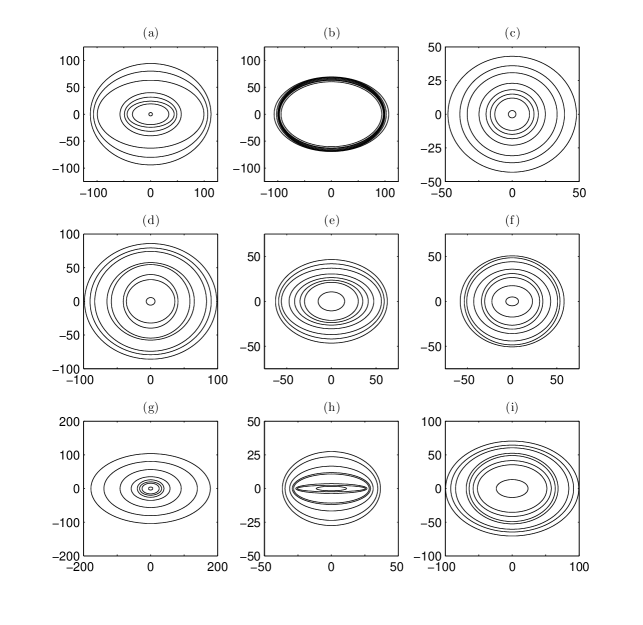
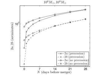
Figure 2 shows the error ellipse evolution for nine examples taken from a sample of computed with , and . We show results for 0, 1, 2, 4, 7, 14, 21, and 28. For each binary, the major axis is plotted on the -axis, while the minor axis is plotted on the -axis; we do not show how each ellipse would be oriented on the sky. The results shown in Figures 2a and 2b were selected by hand from the distribution as examples of contrasting behavior. The binary in Figure 2a shows a dramatic change in the error ellipse with time, especially in the last day before merger. In that day, the binary is localized to an ellipse with and , an area times smaller than at . By contrast, the binary in Figure 2b shows almost no change in the error ellipse over the entire four weeks prior to merger.
These are clearly extreme cases. Other extremes exist, including binaries with a minor axis orders of magnitude smaller than the major axis (see the tail in Fig. 1, right), binaries where the evolution of one or both axes is not strictly monotonic, and binaries which have very large ellipses (essentially filling the sky) for large . (Such cases correspond to binaries which are already well into the LISA band when the mission starts; for large , there is little baseline for the various modulations to encode their position.) To get a sense of more typical behavior, we selected the binaries in Figures 2c – 2i randomly from the distribution. There does not appear to be any “typical” evolution; each binary exhibits some unique features. Most binaries, however, seem to share with the binary in Figure 2a the property that the final day before merger gives much more information on the position than any day before it (albeit to a lesser degree). We will see below that this feature holds for the medians of almost all mass and redshift cases. It is worth noting that although K07 agree with us on most of the other qualitative features of the time dependence, they do not see the dramatic change in the final day of inspiral. As we will discuss in more detail below, this dramatic improvement toward the end of inspiral is due to spin precession physics. This is in good agreement with the expectations of N. Cornish (2005, unpublished) and K07 that spin precession would most dramatically impact the last week or so of inspiral.
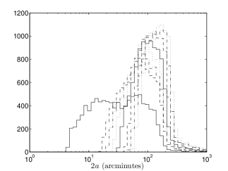
While the evolution of parameter errors for individual binaries is interesting, of more relevance is the evolution of the errors’ distribution. The left panel of Figure 3 shows the time dependence of the distribution of the major axis for our model system of , , and . We can clearly see the evolution to smaller major axis as the binary nears merger. Four weeks before merger, the median major axis is times larger than at merger; this number shrinks to two weeks before merger, one week before, and two days before. As expected from the individual binaries, the most dramatic change in the distribution occurs during the last day before merger. Not only is the median substantially reduced (by a factor of ), but the shape sharply changes. For , the distribution is distinctly peaked, becoming gradually flatter as gets smaller. Over the last day of inspiral, the distribution evolves into the almost entirely flat, slightly bimodal shape first seen in Figure 1. We find that this same behavior holds for all masses and redshift cases of interest: A sharply peaked distribution at evolves into the flatter, sometimes bimodal final distributions described in § 2.4. As the total mass increases, however, the final distributions become so narrow that the shape change is no longer very clear. As we might expect, this transition occurs at smaller total mass for higher .
The right panel of Figure 3 shows the evolution of the minor axis . Again the distribution slowly changes shape over time, with the most drastic change occurring in the last day. Here the final distribution still retains a slight peak, along with the previously discussed long tail of small errors. Interestingly, this tail is present to some degree throughout the evolution. As the total mass increases, the final distribution moves to the right until, as with , the sharp change of shape disappears. The same evolution occurs at higher , again with a shift in the mass scale.

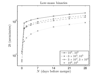
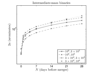


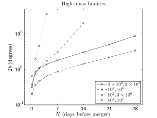
To further understand how the error ellipse evolves, consider Figure 4. Here we show the evolution of the median axes for a wide range of masses (“low,” “intermediate,” and “high”) at . As in Figures 2 and 3, our calculations produce output for 0, 1, 2, 4, 7, 14, 21, and 28; they are connected by lines only to guide the eye. Almost all the cases we present show similar behavior: The ellipses gradually shrink with time before sharply decreasing in size during the final day. Significant deviations from this behavior come from the high-mass binaries, which evolve more drastically at large before settling in to resemble the lower mass curves. This high-mass deviation is an artifact of our choice of maximum . Smaller binaries may spend many months or even years in the LISA band before merger. In those cases, enough signal has already been measured at to locate the binary reasonably well. By contrast, the high-mass binaries spend much less time in band555The two highest mass binaries in Fig. 4 are not even in band a full 28 days. and have not been measured so well by . They have to “catch up” to the smaller mass binaries over the first few weeks of our measurement window. Nearly identical results were found by K07: Figure 2 of K07 plots the evolution of sky position for an intermediate-mass binary from . They find that the measurement accuracy rapidly evolves early in the measurement, with slopes of angular error versus time very similar to what we show in Figure 4 for high-mass binaries.
Although these curves are qualitatively quite similar, there are significant quantitative differences. For example, the evolution of the intermediate-mass binaries is less than that of the low-mass binaries, especially in the last day. The intermediate-mass major axes shrink by a factor of over the entire four-week period, whereas the low-mass axes shrink by a factor of . Another important quantitative difference can be seen by comparing the major and minor axes. We find that the ratio grows with time in most cases, indicating that the minor axis tends to shrink more rapidly than the major axis. The only exceptions are the previously described high-mass cases, in which shrinks during most or all of the inspiral. Presumably the same behavior would also be seen for lower mass binaries at higher values of ; this conclusion is supported by Figure 4 of Kocsis et al. (2007a). For all other cases, at and increases to at . The largest increase is typically in the final day.
What causes this dramatic improvement in the last day of inspiral? Three factors primarily contribute to our ability to localize a source on the sky: modulations due to LISA’s orbital motion, modulations due to spin precession, and S/N accumulated over time. Since LISA moves the same amount in the final day as in any other day, orbital-induced modulations cannot be the cause. A great deal of S/N is accumulated in the last day (typically increasing by a factor of or more), and many parameter errors scale as (S/N)-1. However, K07 demonstrate that sky position and distance errors do not scale as (S/N)-1 in the last few weeks before merger. Our “no precession” code supports their conclusion: The final jump in S/N cannot make up for the lack of orbital modulation over such a short timescale.
The remaining possibility is spin-induced precession. Indeed, we found in Paper I that the number of modulations due to spin precession increases dramatically as the binary approaches merger. This suggests that the improvement we see is due to the impact of precession. To examine this hypothesis, we plot the “precession” and “no precession” results together on the same axes. Figure 5 shows such a plot for a low-mass system and an intermediate-mass system at . We see that at days, the two codes give similar results for localization accuracy. Their predictions gradually diverge as merger is approached. The greatest jump between the two codes occurs on the last day before merger, agreeing with our expectation that precession effects are maximal then. The effect is greater in the low-mass case than in the intermediate-mass case. Similarly, the ratio starts about the same in both codes, growing very slowly until . At this point, it jumps dramatically in the precession code, while staying roughly the same in the no precession code. Interestingly, one effect of precession is that the localization errors track (S/N)-1 rather closely. By breaking the various correlations which made them deviate from (S/N)-1, precession-induced modulations allow the errors to evolve in a manner that is more consistent with our naive expectations.

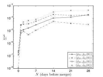
The time evolution of the correlations of interest, those between the sky position and binary orientation, are illustrated in Figure 6. Here we show the off-diagonal components of the covariance matrix (where and ) for the binary in Figure 2a. We found that examining the normalized correlation coefficients can mislead since and are rapidly evolving at the same time as . At large , the two sets of angles are relatively strongly correlated due to degeneracies in the measured waveform (6). However, in the last day before merger, the correlations sharply decrease as precession effects accumulate. The reduction of these correlations coincides with the sudden drop in parameter errors seen in Figure 2 (and, by extension to the entire Monte Carlo run, Figs. 3 – 5).
Finally, we investigate the time evolution of errors in the luminosity distance . Figure 7 shows the distribution of (determined solely by taking into account GW measurement effects) evolving in time for a binary with , , and . We see that in contrast to sky position, the shape of the distribution does not change very much with time. It typically spreads enough to reduce its height, but it maintains a well-defined peak. However, the progression of the median is very similar to the sky position case: It decreases slowly with time until the last day, when it jumps drastically. The evolution of median values of follows tracks very similar in shape to those shown in Figure 4, so we do not show them explicitly.

Table 5 summarizes all of our results on the time evolution of localization. At low redshift, the ability to locate an event on the sky is quite good over much of the mass range even as much as a month in advance of the final merger. In most cases, the localization ellipse at is never larger than about in size, which is comparable to the field of view of proposed future surveys, such as LSST (Tyson et al., 2002). This ability degrades fairly rapidly as redshift increases, especially for larger masses. At , the ellipse can be a few days in advance of merger for small and intermediate masses. At the highest masses, GWs provide very little localization information. Going to makes this even worse; an ellipse of can be found at most a day prior to merger, and only for relatively small mass ranges.
In many cases, is determined so well by GWs that gravitational lensing errors are expected to dominate. As such, the GW-determined values of are essentially irrelevant for locating these binaries in redshift space; lensing will instead determine how well redshifts can be measured. However, in some cases, the intrinsic distance error exceeds the lensing error, so it is worth knowing when the “lensing limit” can be achieved. At , the limit is achieved for most binaries as long as a month before merger. For , the limit is only achieved a few days to a week (depending on mass) before merger; for , intrinsic errors generally exceed the lensing errors even at a day before merger.
| Binary Range | (days) | (deg) | (deg) | |||
|---|---|---|---|---|---|---|
| Low () | aaThese angles are in arcminutes; all others are in degrees. | aaThese angles are in arcminutes; all others are in degrees. | ||||
| aaThese angles are in arcminutes; all others are in degrees. | aaThese angles are in arcminutes; all others are in degrees. | |||||
| aaThese angles are in arcminutes; all others are in degrees. | aaThese angles are in arcminutes; all others are in degrees. | |||||
| aaThese angles are in arcminutes; all others are in degrees. | aaThese angles are in arcminutes; all others are in degrees. | |||||
| Int. () | aaThese angles are in arcminutes; all others are in degrees. | aaThese angles are in arcminutes; all others are in degrees. | ||||
| aaThese angles are in arcminutes; all others are in degrees. | aaThese angles are in arcminutes; all others are in degrees. | |||||
| aaThese angles are in arcminutes; all others are in degrees. | aaThese angles are in arcminutes; all others are in degrees. | |||||
| aaThese angles are in arcminutes; all others are in degrees. | aaThese angles are in arcminutes; all others are in degrees. | |||||
| High () | ||||||
| bbSome very massive systems are excluded from these data. In those cases, the position and distance are very poorly constrained this far in advance of merger. In some cases, the binary is even out of band. | ||||||
| bbSome very massive systems are excluded from these data. In those cases, the position and distance are very poorly constrained this far in advance of merger. In some cases, the binary is even out of band. | ||||||
| Low () | ||||||
| Int. () | ||||||
| High () | ||||||
| bbSome very massive systems are excluded from these data. In those cases, the position and distance are very poorly constrained this far in advance of merger. In some cases, the binary is even out of band. | ||||||
| bbSome very massive systems are excluded from these data. In those cases, the position and distance are very poorly constrained this far in advance of merger. In some cases, the binary is even out of band. | ||||||
| ccAll of the binaries of this mass and redshift are either very poorly measured or completely out of band this far in advance of merger. | ||||||
| Low () | ||||||
| Int. () | ||||||
| bbSome very massive systems are excluded from these data. In those cases, the position and distance are very poorly constrained this far in advance of merger. In some cases, the binary is even out of band. | ||||||
| High () | bbSome very massive systems are excluded from these data. In those cases, the position and distance are very poorly constrained this far in advance of merger. In some cases, the binary is even out of band. | |||||
| bbSome very massive systems are excluded from these data. In those cases, the position and distance are very poorly constrained this far in advance of merger. In some cases, the binary is even out of band. | ||||||
| ccAll of the binaries of this mass and redshift are either very poorly measured or completely out of band this far in advance of merger. |
3.3 Results II: Angular dependence of localization accuracy
We now examine one final interesting property of the errors: their dependence on the sky position of the source. As we design future surveys to find counterparts to MBHB coalescences, it will be important to understand if there is a bias for good (or bad) localization in certain regions of the sky. It is also useful to know in advance whether the “best” regions are likely to be blocked by foreground features such as the Galactic center.
Before discussing this dependence in detail, it is worth reviewing some details of how our Monte Carlo distributions are constructed. As described in § 2.4, in most of our analysis we randomly distribute the sky position of our binaries, drawing from a uniform distribution in and , where and are the polar and azimuthal angles of a binary in solar system barycenter coordinates. We also randomly choose our binaries’ final merger time. In this section, rather than distributing the sky position, we examine parameter accuracies for particular given positions; all other Monte Carlo parameters are distributed as usual. Because we continue to randomly distribute the final merger time, the relative azimuth between a binary’s sky position and LISA’s orbital position at merger, , remains randomly distributed. As such, we expect our analysis to effectively average over , washing out any strong dependence on this angle in our analysis.
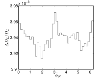
We begin by examining the dependence of errors on . We evenly divide the range into 40 bins and run a Monte Carlo simulation with points in each. That is, we pick only from the bin range, but we pick all other random parameters in the usual manner. The results for a representative binary (, and ) are shown in Figure 8.
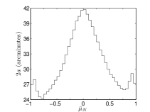

Note that all of the error distributions are symmetrically peaked around the plane of LISA’s orbit (). Any slight asymmetry is due only to statistical effects. This is reassuring; LISA should not favor one hemisphere over the other. There is also additional structure that is parameter dependent. At its peak, the major axis is almost greater than the position-averaged median value666Note that the position-averaged medians quoted here are slightly different from those quoted in Table 1, since this sample has 40 times more points. of . It then decreases with and reaches a minimum of about for . Finally, there are subpeaks near the ecliptic poles, although they still lie below the position-averaged median. The dependence of the minor axis on angle is even more dramatic. At its peak, differs from the position-averaged median of by over . Just like the major axis, it drops to a minimum, but it does so more rapidly. The minimum also occurs at a slightly larger value of than for . The minor axis also shows fairly strong subpeaks near the ecliptic poles, with values higher than the position-averaged median.
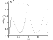
The luminosity distance errors behave slightly differently. First of all, the variation with is weaker than for the sky position: At the central peak, is only greater than its position-averaged median value (). In addition, while the distribution again peaks near the poles, it does so at a smaller value of . (In fact, the peaks occur very close to where sky position errors are minimized.)
By binning the data sets developed for Paper I, we were able to confirm this behavior over a wide range of masses and redshifts, albeit with poorer statistics: binaries in total, rather than per bin. Thanks to the poorer statistics, we cannot resolve the small polar subpeaks in the distribution of . In addition, in some cases it appears that the side peaks can be larger than the central peak in the distribution of . Aside from these minor variations, the shapes and relative amplitudes seen in these distributions hold robustly over all masses and redshifts we considered.


We next investigate the dependence of the errors on the azimuthal angle . To improve the statistics, we now calculate binaries in each bin; the results are shown in Figure 9. The errors have a very weak (although nonzero) dependence on : The maximum deviation from the overall median is only . This is to be expected; as discussed at the beginning of this section, the randomness of our binaries’ merger times effectively averages over azimuth. If we did not average over azimuth in this way, we would expect a moderately strong -dependence due to the functional form of LISA’s response to GWs. Even after averaging this dependence away, we might expect some residual structure due to the “rolling” motion of the LISA constellation. The phase associated with LISA’s roll angle puts an additional oscillation on the measured waves (see the -dependence in eqs. [47] and [48] of K07, where encodes the roll angle), and we do not average over this angle. Indeed, on close inspection, we can make out roughly two peaks in each plot in Figure 9 (although the statistics are still too poor to resolve them clearly), consistent with the and behavior shown in K07. For comparison, we also examined the -dependence for this mass and redshift with precession “turned off.” The oscillatory behavior appears very clearly in this case. Because of the weakness of the behavior, we were unable to easily check it for other masses and redshifts.
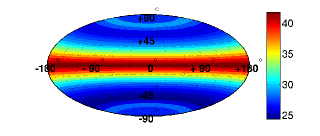
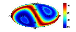
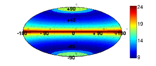
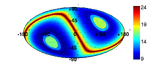
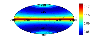
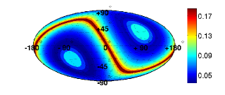
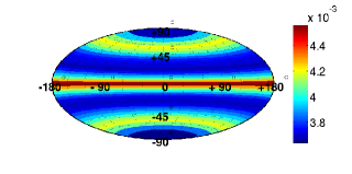
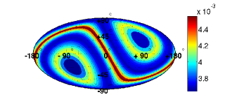
Finally, to give an overall sense as to how localization varies on the sky, we present in Figure 10 sky maps of the median major axis , minor axis , localization ellipse area , and distance accuracy . We show these data both in ecliptic and Galactic coordinates. Note that most of the region of small error lies outside of the Galactic plane. This potentially bodes well for searches for MBHB electromagnetic counterparts — the regions where instruments like LISA “see” most sharply are less likely to be hidden by foreground features. Certain portions of the sky that LISA sees well will be easier to search telescopically than others. It will be an important task for future surveys over all electromagnetic bands to identify regions that are particularly amenable to finding counterparts to MBHB events.
4 Summary and conclusions
As discussed at length in Paper I, accounting for the general relativistic precession of the angular momentum vectors in an MBHB system has a dramatic impact on what we can learn by observing the system’s gravitational waves. Spin-induced precession breaks degeneracies among different parameters, making it possible to measure them more accurately than they could be determined if precession were not present. This has a particularly important impact on our ability to locate such a binary on the sky and to determine its luminosity distance — the degeneracy between sky angles, distance, and orientation angles is severe in the absence of precession.
Our analysis shows that the improvement that precession imparts to measurement accumulates fairly slowly. In using one code which includes the impact of spin precession and a second which neglects this effect, we find little difference in the accuracy with which GWs determine sky position and distance for times more than a few days in advance of the final merger. The difference between the two codes grows quite rapidly in these final days. In the last day alone, the localization ellipse area decreases by a factor of (up to in a few low-mass systems) when precession effects are included. Distance determination is likewise improved by factors of in that final day.
Not all of the precession effects occur in the final days. We saw in Figure 3 that the long tail of small minor axes can be seen, to some degree, throughout the inspiral. We could get lucky and find a binary with a very small value of weeks before merger. But the improvement in the median that we found in Paper I appears to take effect only in the final days of inspiral. Therefore, while precession may in fact help improve the final localization of a coalescing binary by a factor of in each direction, it will not be much help in advanced localization of a typical binary.
Nevertheless, the pixel sizes that we find are small enough that future surveys should not have too much trouble searching the region identified by GWs, at least over certain ranges of mass and redshift. At , the GW localization ellipse is or smaller for most binaries as early as a month in advance of merger. (At high masses, the ellipse can be substantially larger than this a month before merger, but it shrinks rapidly, reaching a comparable size weeks before merger.) This bodes well for future surveys with large fields of view that are likely to search the GW pixel for counterparts. In addition, GWs determine the source luminosity distance so well that the distance errors we find are essentially irrelevant — gravitational lensing will dominate the distance error budget for all but the highest masses.
As redshift increases, the GW pixel rapidly degrades, particularly for the largest masses. Let us adopt (the approximate LSST field of view) as a benchmark localization for which counterpart searches may be contemplated. At , this benchmark is reached at merger for almost the entire range of masses we considered. As little as a day in advance of merger, however, some of the least massive and most massive systems are out of this regime. One week prior to merger, the most massive systems are barely located at all (ellipses hundreds of square degrees or larger). The intermediate masses do best, but even in their cases the positions are determined with accuracy no earlier than a few days in advance of merger. The resolution degrades further at higher redshift. At , systems with are not located more accurately than even at merger. Smaller systems are located within at merger, but very few are at this accuracy even one day in advance of merger. The luminosity distance errors also increase, so much that they exceed lensing errors a few days to a week before merger at , and only a day before merger at . This degradation hurts the ability to search for counterparts by redshift and subsequently use them as standard candles.
Our main conclusion is that future surveys are likely to have good advanced knowledge (a few days to one month) of the location of MBHB coalescences at low redshift (), but only a day’s notice at most at higher redshift (). This conclusion may be excessively pessimistic. As mentioned earlier, recent work examining the importance of subleading harmonics of MBHB GWs is finding that including harmonics beyond the leading quadrupole has an important effect on the final accuracy of position determination (Arun et al., 2007; Trias & Sintes, 2008). For most masses, these analyses show a factor of a few improvement in position, comparable to the improvement that we find when spin precession is added to the waveform model. For high-mass systems, the higher harmonics increase the (previously small) overlap with the LISA band; consequently, the improvement can be much larger, up to 2 or 3 orders of magnitude in area. Since these two improvements arise from very different physical effects, it is likely that their separate improvements can be combined for an overall improvement significantly better than each effect on its own. We plan to test this in future work (which is just now getting underway).
Finally, we have also studied the sky position dependence of LISA’s ability to localize sources. We have found that the regions of best localization lie fairly far out of the Galactic plane. However, as emphasized by N. Cornish (2007, private communication), a proper anisotropic confusion background might impact this dependence. In our calculations, we have assumed an isotropic background, neglecting the likely spatial distribution of Galactic binaries. Properly accounting for this background is likely to strengthen our conclusion that LISA’s ability to “see” is best for MBHB sources out of the Galactic plane.
References
- Apostolatos et al. (1994) Apostolatos, T. A., Cutler, C., Sussman, G. J., & Thorne, K. S. 1994, Phys. Rev. D, 49, 6274
- Armitage & Natarajan (2002) Armitage, P. J., & Natarajan, P. 2002, ApJ, 567, L9
- Arun et al. (2007) Arun, K. G., Iyer, B. R., Sathyaprakash, B. S., Sinha, S., & Van Den Broeck, C. 2007, Phys. Rev. D, 76, 104016
- Berti et al. (2005) Berti, E., Buonanno, A., & Will, C. M. 2005, Phys. Rev. D, 71, 084025
- Blanchet (2006) Blanchet, L. 2006, Living Rev. Relativ., 9, 4
- Blanchet et al. (1995) Blanchet, L., Damour, T., Iyer, B. R., Will, C. M., & Wiseman, A. G. 1995, Phys. Rev. Lett., 74, 3515
- Bode & Phinney (2007) Bode, N., & Phinney, E. S. 2007, APS Abstr., http://meetings.aps.org/link/BAPS.2007.APR.S1.10
- Buonanno et al. (2007) Buonanno, A., Cook, G. B., & Pretorius, F. 2007, Phys. Rev. D, 75, 124018
- Cutler (1998) Cutler, C. 1998, Phys. Rev. D, 57, 7089
- Cutler & Flanagan (1994) Cutler, C., & Flanagan, É. É. 1994, Phys. Rev. D, 49, 2658
- Dalal et al. (2003) Dalal, N., Holz, D. E., Chen, X., & Frieman, J. A. 2003, ApJ, 585, L11
- Dotti et al. (2006) Dotti, M., Salvaterra, R., Sesana, A., Colpi, M., & Haardt, F. 2006, MNRAS, 372, 869
- Farmer & Phinney (2003) Farmer, A. J., & Phinney, E. S. 2003, MNRAS, 346, 1197
- Ferrarese & Merritt (2000) Ferrarese, L., & Merritt, D. 2000, ApJ, 539, L9
- Finn (1992) Finn, L. S. 1992, Phys. Rev. D, 46, 5236
- Frieman (1997) Frieman, J. A. 1997, Comments Astrophys., 18, 323
- Gebhardt et al. (2000) Gebhardt, K., et al. 2000, ApJ, 539, L13
- Hellings & Moore (2003) Hellings, R. W., & Moore, T. A. 2003, Classical Quantum Gravity, 20, S181
- Holz (1998) Holz, D. E. 1998, ApJ, 506, L1
- Holz & Hughes (2005) Holz, D. E., & Hughes, S. A. 2005, ApJ, 629, 15
- Holz & Wald (1998) Holz, D. E., & Wald, R. M. 1998, Phys. Rev. D, 58, 063501
- Hughes (2002) Hughes, S. A. 2002, MNRAS, 331, 805
- Kidder (1995) Kidder, L. E. 1995, Phys. Rev. D, 52, 821
- Kocsis et al. (2006) Kocsis, B., Frei, Z., Haiman, Z., & Menou, K. 2006, ApJ, 637, 27
- Kocsis et al. (2007a) Kocsis, B., Haiman, Z., & Menou, K. 2007a, ApJ, submitted (arXiv:0712.1144)
- Kocsis et al. (2007b) Kocsis, B., Haiman, Z., Menou, K., & Frei, Z. 2007b, Phys. Rev. D, 76, 022003 (K07)
- Lang & Hughes (2006) Lang, R. N., & Hughes, S. A. 2006, Phys. Rev. D, 74, 122001 (Paper I)
- Larson et al. (2000) Larson, S. L., Hiscock, W. A., & Hellings, R. W. 2000, Phys. Rev. D, 62, 062001
- Micic et al. (2007) Micic, M., Holley-Bockelmann, K., Sigurdsson, S., & Abel, T. 2007, MNRAS, 380, 1533
- Milosavljević & Phinney (2005) Milosavljević, M., & Phinney, E. S. 2005, ApJ, 622, L93
- Nelemans et al. (2001) Nelemans, G., Yungelson, L. R., & Portegies Zwart, S. F. 2001, A&A, 375, 890
- Pan et al. (2008) Pan, Y., Buonanno, A., Baker, J. G., Centrella, J., Kelly, B. J., McWilliams, S. T., Pretorius, F., & van Meter, J. R. 2008, Phys. Rev. D, 77, 024014
- Phillips (1993) Phillips, M. M. 1993 ApJ, 413, L105
- Poisson & Will (1995) Poisson, E., & Will, C. M. 1995, Phys. Rev. D, 52, 848
- Riess et al. (1995) Riess, A. G., Press, W. H., & Kirshner, R. P. 1995, ApJ, 438, L17
- Tyson et al. (2002) Tyson, J. A., & the LSST Collaboration 2002, Proc. SPIE Int. Soc. Opt. Eng., 4836, 10
- Vecchio (2004) Vecchio, A. 2004, Phys. Rev. D, 70, 042001
- Sesana et al. (2007) Sesana, A., Volonteri, M., & Haardt, F. 2007, MNRAS, 377, 1711
- Trias & Sintes (2008) Trias, M., & Sintes, A. M. 2008, Phys. Rev. D, 77, 024030
- Wang et al. (2003) Wang, L., Goldhaber, G., Aldering, G., & Perlmutter, S. 2003, ApJ, 590, 944
- Wang et al. (2002) Wang, Y., Holz, D. E., & Munshi, D. 2002, ApJ, 572, L15
- Will & Wiseman (1996) Will, C. M., & Wiseman, A. G. 1996, Phys. Rev. D, 54, 4813