The Galaxy Content of SDSS Clusters and Groups
Abstract
Imaging data from the Sloan Digital Sky Survey are used to characterize the population of galaxies in groups and clusters detected with the MaxBCG algorithm. We investigate the dependence of Brightest Cluster Galaxy (BCG) luminosity, and the distributions of satellite galaxy luminosity and satellite color, on cluster properties over the redshift range . The size of the dataset allows us to make measurements in many bins of cluster richness, radius and redshift. We find that, within of clusters with mass above , the luminosity function of both red and blue satellites is only weakly dependent on richness. We further find that the shape of the satellite luminosity function does not depend on cluster-centric distance for magnitudes brighter than - 5log . However, the mix of faint red and blue galaxies changes dramatically. The satellite red fraction is dependent on cluster-centric distance, galaxy luminosity and cluster mass, and also increases by 5% between redshifts 0.28 and 0.2, independent of richness. We find that BCG luminosity is tightly correlated with cluster richness, scaling as , and has a Gaussian distribution at fixed richness, with for massive clusters. The ratios of BCG luminosity to total cluster luminosity and characteristic satellite luminosity scale strongly with cluster richness: in richer systems, BCGs contribute a smaller fraction of the total light, but are brighter compared to typical satellites. This study demonstrates the power of cross-correlation techniques for measuring galaxy populations in purely photometric data.
Subject headings:
galaxies: clusters — galaxies: evolution — galaxies: halos — cosmology: observations1. Introduction
Clusters of galaxies are important systems for studying both galaxy evolution and cosmology. Used as laboratories with well-defined environments, these massive objects are a tool for investigating processes that influence galaxies’ physical characteristics. Used as tracers of the underlying mass distribution, they are a tool for investigating the evolution of structure and the nature of dark energy in the Universe. These objectives are closely linked: cosmological studies require accurate knowledge of cluster selection and redshift- and mass-observable relations, and these facts are directly related the evolutionary properties of the cluster galaxy population.
In the context of galaxy evolution, the high-density environment of galaxy clusters is a particularly interesting place to examine the galaxy population. Several studies have suggested substantial galaxy transformation in such environments. Galaxy morphology, star-formation rate, and luminosity have long been known to depend on cluster properties and to depart significantly from the cosmological average (e.g., Hubble, 1926; Abell, 1962; Oemler, 1974; Dressler, 1980). Historically, the cluster galaxy content has been quantified by the luminosity function (LF) and type fraction (such as the late-type or blue fraction). Measurement of these quantities as a function of cluster mass, redshift, and distance from the cluster center provides insight into the underlying physical mechanisms responsible for these trends.
While the LF is primarily a decreasing function of luminosity, galaxies are bimodal in color and spectral type, with red, early-type galaxies displaying little ongoing star formation, and blue, late-type galaxies exhibiting signs of recent star formation (e.g., Strateva et al., 2001; Baldry et al., 2004; Bell et al., 2004; Menanteau et al., 2006; Blanton et al., 2005a). This bimodality was in place by at the latest and may provide a signpost of galaxy transformation (e.g., Faber et al., 2007). Although this bimodality persists in all environments, the fraction of galaxies in each class (a.k.a. the red and blue fractions) changes systematically with local density; this trend is the so-called morphology-density relationship (Oemler, 1974; Dressler, 1980; Dressler et al., 1997; Smith et al., 2005). In recent large galaxy surveys this work has been extended to show that a wide range of galaxy properties, including morphology, star-formation rate, and color, depend on local density (Gómez et al., 2003; Balogh et al., 2004a, b; Hogg et al., 2004; Kauffmann et al., 2004; Tovmassian et al., 2004; Blanton et al., 2005a; Christlein & Zabludoff, 2005; Croton et al., 2005; Rojas et al., 2005; Cooper et al., 2006; Mandelbaum et al., 2006; Cooper et al., 2007).
The advent of large galaxy surveys has made it possible to place observational constraints on both the type fraction and the LF as a function of cluster mass (the conditional luminosity function, CLF), and to further investigate how these quantities depend on other variables. In the Sloan Digital Sky Survey (York et al., 2000, SDSS), Goto et al. (2002) and Hansen et al. (2005) examined the LF as a function of cluster richness and cluster-centric distance for systems found in the SDSS Early Data Release, and Weinmann et al. (2006b) measured the CLF measured from a group catalog derived from the spectroscopic sample of SDSS DR2. Using the 2dF Galaxy Redshift Survey, De Propris et al. (2003) and Robotham et al. (2006) compared the LF in high- and low-mass systems; a similar study was performed with a sample of 93 X-ray selected clusters (Lin et al., 2004). The dependence of the LF on galaxy color has been recently investigated (Popesso et al., 2005) as has the galaxy type fraction (Goto et al., 2003; De Propris et al., 2004) for clusters in these large surveys.
The type fraction of galaxies in clusters depends on both cluster richness and redshift: the fraction of star-forming galaxies at fixed local density is larger at higher redshift, an effect known as the Butcher–Oemler effect (Butcher & Oemler, 1978, 1984). This effect is now well-documented, if not entirely well-explained, in clusters over a wide range of masses by studies of the blue fraction, or its converse, the red fraction (Rakos & Schombert, 1995; Margoniner & de Carvalho, 2000; Ellingson et al., 2001; Kodama & Bower, 2001; Margoniner et al., 2001; De Propris et al., 2004; Martínez et al., 2006; Gerke et al., 2007). Other indicators of galaxy state, including galaxy morphology and emission line strength, also show a trend with redshift (Allington-Smith et al., 1993; Oemler et al., 1997; Balogh et al., 1997; Couch et al., 1998; van Dokkum et al., 2000; Fasano et al., 2000; Lubin et al., 2002; Goto et al., 2003; Treu et al., 2003; Wilman et al., 2005; Poggianti et al., 2006; Desai et al., 2007; van der Wel et al., 2007). However, few samples to date have had both large numbers of systems and well-understood mass proxies, so the dynamical range and mass resolution of these previous works has been somewhat limited.
Another characteristic of galaxy clusters is the presence of a highly-luminous galaxy near the cluster center — the Brightest Cluster Galaxy (BCG). In addition to being extraordinarily luminous, BCGs differ in a number of ways from other cluster members: they tend to have extended light profiles (Matthews et al., 1964; Tonry, 1987; Schombert, 1988; Gonzalez et al., 2000, 2003), larger size at fixed luminosity than other early types (Bernardi et al., 2007, and references therein) and may contain a larger fraction of dark matter than typical galaxies (e.g., Mandelbaum et al., 2006; von der Linden et al., 2007). Also, while the traditional fitting function to the LF of Schechter (1976) provides a good fit for satellite galaxies, BCGs follow a different distribution, causing the so-called “bright end bump” (e.g., Hansen et al., 2005). This difference between the BCG and other satellites in a cluster is also manifested in the luminosity gap statistic, the difference in luminosity between the BCG and the next brightest cluster member, which may be indicative of the special accretion history of BCGs (Ostriker & Tremaine, 1975; Tremaine & Richstone, 1977; Loh & Strauss, 2006). BCGs are also distinct from other galaxies with similar mass that are not at the center of cluster-sized potential wells (von der Linden et al., 2007). Indeed, the properties of BCGs seem to be closely linked to properties of their host clusters (Sandage & Hardy, 1973; Schneider et al., 1983; Schombert, 1988; Edge & Stewart, 1991; Brough et al., 2002; De Grandi et al., 2004; Brough et al., 2005; Loh & Strauss, 2006), including to the masses of their parent halos (Lin & Mohr, 2004; Mandelbaum et al., 2006; Zheng et al., 2007). The outer light profile of BCGs often merges smoothly with the diffuse intra-cluster light (ICL), suggesting again a coupling between the BCG and the host halo (Gonzalez et al., 2005). Generally the BCG+ICL light is closely linked with cluster mass (Zibetti et al., 2005; Conroy et al., 2007; Purcell et al., 2007; Gonzalez et al., 2007). As BCGs have properties different from those of the rest of the cluster members, BCGs and satellites are often analyzed separately, and we follow this convention here.
It is expected that the properties of cluster galaxies are closely tied to the merging and accretion history of their parent dark matter halos. Current models based on Cold Dark Matter (CDM) suggest that the stars in BCGs were formed in dense peaks quite early but that the BCGs were assembled in a series of galaxy merging events that continue until relatively recent times (e.g. Aragon-Salamanca et al., 1998; Dubinski, 1998; Gao et al., 2004; Boylan-Kolchin et al., 2006; De Lucia & Blaizot, 2007). Satellite galaxies in clusters are now generally understood to be hosted by smaller dark matter halos that have merged into the parent halo. Several features of the observed cluster galaxy populations can be understood based on the assembly history of the parent halo (e.g., Poggianti et al., 2006; Tasitsiomi et al., 2007). One such characterization is the core distinction between central galaxies and satellites: the central concentrations of mass and light in massive halos continue to build up while the growth of satellite systems is halted upon accretion. BCG luminosity, and the correlations between this luminosity and both cluster mass and satellite properties, can thus provide insight into the assembly histories of clusters.
The merger history of dark matter halos alone is not enough to account for the bimodality in galaxy properties and its dependence on redshift and environment. Several physical processes have been proposed to transform star-forming galaxies into the typical cluster galaxies on the red sequence. Although the relative strengths of these processes are still hotly debated, a consensus is emerging that the main transformation mechanisms are related to the mass of the host halo and whether (and for how long) the galaxy has been a satellite within a larger system. Among the suggested transformation mechanisms, some are expected to be most effective in rich clusters, such as ram-pressure stripping (Gunn & Gott, 1972), interaction with the cluster potential (Byrd & Valtonen, 1990) and high-velocity close encounters (“harassment;” Moore et al., 1996). However, studies of very poor systems have shown that the environmental dependence of galaxy properties is not limited to the richest objects (e.g., Zabludoff & Mulchaey, 1998; Weinmann et al., 2006a; Gerke et al., 2007). Processes that can operate efficiently in low velocity dispersion systems therefore must also play a role in shaping the galaxy population: e.g., galaxy mergers (Toomre & Toomre, 1972) and “strangulation,” a cutoff to gas accretion onto galaxy disks by stripping or AGN feedback (Larson et al., 1980; Balogh et al., 2000; Croton et al., 2006). It is likely that some combination of these effects is at work. Distinguishing their relative significance requires precisely quantifying cluster galaxy properties over a wide range of masses and as a function of cluster-centric distance. These data will provide information on both the assembly histories of clusters and on the physical mechanisms that trigger and quench star formation.
Models of galaxy evolution in a cosmological context most readily predict galaxy properties as a function of halo mass rather than cluster observables. In order to make these comparisons, a reliable mass–observable relationship is a prerequisite. In addition, there is consensus that the luminosity function and type fraction both depend on a number of variables, complicating detailed comparison between clusters of different mass. For example, the cluster galaxy LF depends on cluster-centric distance, and the size of the bound regions of clusters scales with mass. In order to make physically meaningful comparisons between LFs of different mass clusters, an aperture scaled to the bound region is therefore preferable to a fixed metric aperture. With recent extensive surveys providing well-calibrated cluster catalogs spanning a wide range in mass, it is possible to examine in detail the dependence of the cluster galaxy population on several cluster and galaxy properties simultaneously.
Large, homogeneous photometric surveys such as the SDSS provide rich data with which to characterize the cluster galaxy population. These data have been used to define large, robust, clean samples of galaxy clusters with accurate photometric redshifts. These samples are sizable enough to split on several variables allowing detailed statistical exploration of the galaxy populations in clusters. Currently, the largest sample of clusters available is the MaxBCG catalog from the Sloan Digital Sky Survey (Koester et al., 2007b). The selection effects of the cluster-finding algorithm are well understood (Koester et al., 2007a; Rozo et al., 2007a), and there are a number of studies exploring the mass–richness relationship for these objects (Rozo et al., 2007b; Becker et al., 2007; Sheldon et al., 2007a; Johnston et al., 2007b; Rykoff et al., 2007). In this work, we convert cluster richness to cluster mass using weak lensing measurements of the MaxBCG mass–richness relation (Sheldon et al., 2007a; Johnston et al., 2007b). The quality and quantity of these data allow for detailed measurements of a variety of cluster galaxy properties as a function of cluster mass and radius. For satellite galaxies we then measure the luminosity function of all, red, and blue satellites conditional on both mass and cluster radius, and investigate the dependence of the red fraction of satellites on cluster mass, redshift, galaxy luminosity and distance from cluster center; for BCGs we quantify the dependence on cluster mass of both the BCG luminosity and the relationship between the BCG luminosity and satellite galaxy luminosities. Although this sample of clusters extends only to , these objects provide a valuable low-redshift baseline with which higher redshift samples may be compared.
In this paper we use a statistical background-subtraction technique to measure mean galaxy properties over a wide range of color and luminosity in MaxBCG clusters. We average the signal from many clusters binned by cluster properties, and statistically subtract the contribution from random galaxies along the line of sight. This method of cross-correlating clusters with the galaxy population provides very precise statistical measurements, and allows us to study blue and low luminosity galaxies that are indistinguishable from the background in individual clusters. We test the background-correction algorithm by running the full analysis on realistic mock catalogs, and find that we are able to robustly recover 3D cluster properties using these methods. The statistical techniques presented here for background correction of photometric data will be directly applicable to future large multi-band imaging programs, including the Dark Energy Survey (DES111http://www.darkenergysurvey.org, Abbott & The DES Collaboration, 2005) and the Large Synoptic Survey Telescope (LSST222http://www.lsst.org, Tyson, 2002) and the Panoramic Survey Telescope & Rapid Response System (Pan-STARRS333http://pan-starrs.ifa.hawaii.edu, Kaiser et al., 2002) and will be essential for leveraging these data to provide the desired insights into cosmology and galaxy evolution.
The paper is organized as follows: in § 2 we describe the SDSS and simulation data used; we present the stacking and background-correction method in § 3. Our primary results are given in § 4: § 4.1 presents the luminosity and color characteristics of the satellite population, while § 4.2 discusses the BCG population. A summary and discussion of the implications of the results is given in § 5.
The notation used for cluster-related variables in previous MaxBCG work includes defining and as the counts and -band luminosity of red-sequence galaxies within the measurement aperture of the cluster finder and with L . We note that as the aperture for cluster finding was determined with a previous definition of richness, it is not strictly the true value of for these systems (in fact, it is larger), and only red galaxies are included in these definitions. In this work we will refer to the total excess luminosity associated with the light from galaxies of all colors above a luminosity threshold and within the measured of these systems as . In addition, we follow the standard convention of using to to denote projected, 2D radii and to refer to deprojected, 3D radii. Where necessary for computing distances, we assume a flat, LCDM cosmology with H km s-1 Mpc-1, , and matter density .
2. Data
We use the photometric data of the Sloan Digital Sky Survey (SDSS) Data Release 4. The SDSS data were obtained using a specially-designed 2.5-m telescope (Gunn et al., 2006), operated in drift-scan mode in five bandpasses () to a limiting magnitude of (Fukugita et al., 1996; Gunn et al., 1998; Lupton et al., in preparation; Hogg et al., 2001; Smith et al., 2002). The survey covers much of the North Galactic Cap and a small, repeatedly-scanned region in the South. Apparent magnitudes are corrected for Galactic extinction using the maps of Schlegel et al. (1998). Photometric errors at bright magnitudes are , limited by systematic uncertainty (Ivezić et al., 2004); astrometric errors are typically smaller than 50 mas per coordinate (Pier et al., 2003). Further details of the SDSS data may be found in the most recent data release paper of Adelman-McCarthy et al. (2007).
With these data, we define a catalog of galaxies, then run our cluster-finding algorithm on this list to produce a catalog of galaxy clusters. The set of clusters and galaxies are then jointly analyzed to determine the binned correlation function measurements used in this work to describe the galaxy population associated with clusters. In this section, we describe the galaxy and cluster catalogs.
2.1. Galaxy Sample
Our photometric galaxy catalog was generated by applying the Bayesian star-galaxy separation method developed in Scranton et al. (2002) to the full set of SDSS data. The primary source of confusion in star-galaxy separation at faint magnitudes is shot noise, which causes stars to scatter out of the stellar locus and galaxies to scatter into the stellar locus. The Scranton et al. (2002) method uses knowledge about the underlying size distribution of objects as a function of apparent magnitude and seeing to assign a probability of being a galaxy to each object. We examined objects from the repeatedly scanned SDSS southern stripe and co-added the fluxes from different exposures at the catalog level to provide more precise sizes and magnitudes. Using regions with at least 20 scans, we selected objects on single exposures with typical observing conditions, but characterized their size distribution as a function of magnitude and seeing with the co-add. From these distributions we generated a galaxy probability for every object in the survey. The resulting distribution is highly peaked at probabilities 0 and 1, such that 0.8 results in a highly pure sample of galaxies. We then searched the resultant catalog of galaxies for systems that are likely to be clusters of galaxies using the MaxBCG algorithm described briefly below and in detail in Koester et al. (2007b).
For characterizing the galaxy population in clusters, we restrict the galaxy sample to be volume and magnitude limited for by including only those galaxies brighter than an appropriate threshold. Expressed as a luminosity K-corrected to redshift (see § 3.4), this lower -band luminosity limit is . At , this value corresponds to an apparent magnitude limit of , and color limits of and . All magnitudes are SDSS model magnitudes. Uncertainties on the measurements are sufficiently small so that the typical signal-to-noise is greater than 30 until beyond redshift 0.3. Galaxy colors are therefore robustly measured (Smail et al., 1995; Bernstein et al., 2002; Benítez et al., 2004) over the full redshift range considered here.
2.2. Cluster Sample
Clusters were identified using the MaxBCG cluster finder of Koester et al. (2007b). This algorithm identifies clusters by the presence of a BCG and a red sequence, and provides an excellent photometric redshift for each system. The scatter in redshift is for our full richness and redshift range and for . The cluster center is defined to be the position of the BCG. The cluster richness, , is defined as the number of red galaxies with rest frame -band luminosity in an aperture that scales with , and is an excellent mass proxy, as discussed below. The catalog of systems with 10 was presented in Koester et al. (2007a); in this work we use systems with 3.
The MaxBCG cluster finder was trained using known BCGs and luminous red galaxies, and as we will consider whether the resulting BCG population is being constrained by these priors, we review the procedure here. Specifically, when constructing the likelihood of a galaxy to be a BCG, the algorithm places priors on observed and colors and -band magnitude. The model BCG color–redshift and magnitude–redshift relationships are taken from the distribution of bright LRG galaxies, then refined based on examination of 100 visually identified BCGs in rich clusters. The BCG likelihood, , is specified to be
| (1) |
(Koester et al., 2007b, Equation 11), where the width of the prior on BCG -band magnitude is 0.3mag, taken from Loh & Strauss (2006). In addition, BCGs are required to be brighter than 0.4 ( at ). The distributions and are narrow Gaussians in color; the width of each includes both the intrinsic width of the E/S0 ridgeline (0.05 for and 0.06 for ) and the error in the measured color for the galaxy in question. In practice, the narrow color priors provide a much stronger constraint in identifying likely BCGs than does the magnitude prior, and for the majority of cases, the BCG is clearly defined by the color criteria. The BCG magnitude likelihood has an appreciable effect only for the cases where the choice of BCG is ambiguous.
The selection function of the MaxBCG algorithm was investigated by Koester et al. (2007b) and Rozo et al. (2007a), who showed that this sample of clusters is over 90% complete and pure for . For sytems, the completeness and purity rates are 97% or better. The completeness and purity were quantified by comparing clusters identified in realistic mock galaxy catalogs (Wechsler et al., 2007) to their host halos. We did not wish to use unresolved halos in our comparisons, so for lower richness values ( ), the completeness and purity are less well quantified. It is likely that the lowest-richness systems are less pure and complete, not only because of statistical considerations but also because the lower richness systems, with just a few red galaxies in close proximity, are not necessarily representative of all systems in the equivalent mass range. Higher resolution simulations will be necessary to quantify this selection in detail; however, we can learn about the statistical properties of these systems even if they are a biased population compared to dark matter halos. We thus include them in this study, but for the purpose of fitting relationships of galaxy properties as a function of cluster richness or mass, we restrict the sample to , where the catalog is known to be both highly complete and pure.
We use clusters in the redshift range 0.1 0.3; there are 165,597 objects identified with 3, of which 13,823 have .
2.3. Average Galaxy Properties at
Below, we compare our derived cluster galaxy population statistics to similar statistics for the mean of galaxies in all environments, which we will refer to as the cosmological, or universal, average. To calculate these average galaxy statistics, we use the New York University Value-Added Galaxy Catalog (NYU-VAGC Blanton et al., 2005b) of the SDSS spectroscopic sample, whose median redshift is , evolved to . The details of constructing this sample are discussed in Sheldon et al. (2007b). By applying the same luminosity and color cuts to this sample as we do to any given set of cluster galaxies (e.g., to determine the density of red, bright galaxies), we estimate the universal average values of a comparable “field” sample. We do not undertake a detailed study of this population here, but just present the average values for general comparison with the recovered cluster values. For reference, from fitting a Schechter function to this sample, we find the global value of evolved to to be .
3. Method
In this section, we describe how we characterize the radial, luminosity, and color distribution of galaxies that are associated with clusters. In § 3.1 we review the estimator used to determine the distribution of cluster galaxies; §§ 3.2 through 3.5 discuss the technical details of characterizing the survey geometry and redshift distributions, performing K-corrections, and determining and . We describe a check to the background correction with a mock galaxy catalog in § 3.6.
We can only reliably determine cluster membership for individual clusters in this purely photometric sample for red, relatively high luminosity galaxies. We nonetheless can accurately characterize the full cluster galaxy population by statistically correcting for galaxies aligned by chance along the line of sight. We perform this correction not on individual clusters, but for ensembles binned together based on their observable properties, such as richness or redshift. We do not recover the properties of individual clusters, but rather properties of the average cluster. In this sense we measure the cross-correlation between clusters and the galaxy population.
If the average stacked cluster is spherically symmetric, we can invert the projected densities to recover the 3D profile. This assumption is true for a homogeneous and isotropoic universe, as long as the cluster finder does not introduce anisotropies: for example, choosing preferentially systems elongated along the line of sight.
To recover the K-corrected luminosities of the average galaxy population, we K-correct galaxies along both the cluster line-of-sight and the random lines-of-sight to the redshift of the cluster, regardless of their true redshifts. After background subtraction, galaxies at redshifts different from the cluster are removed from the counts, and so this inaccuracy does not persist in our final measurements.
A correlation function-based approach is straightforward to implement and interpret, and takes advantage of the full dataset for background correction. This method is in contrast to using a “local” background correction estimate from, for example, counting galaxies in a large annulus around each cluster, as has been done in studies of more limited area. As there is mass and light correlated with clusters out to many times the virial radius, a local background estimate is likely to result in a biased estimate of the true galaxy population in clusters. Masjedi et al. (2006) implemented the use of a correlation function-based estimator to investigate galaxies correlated with the SDSS LRG sample, and here we extend this technique to examine galaxies associated MaxBCG clusters. This estimator is a powerful tool, but requires a significant amount of computation for the large number (here 2.7 billion) of pairs that must be considered.
3.1. Cluster-galaxy Correlations
We follow the method of Masjedi et al. (2006) to estimate the mean number density and luminosity density of galaxies associated with clusters. This method essentially calculates a correlation function with units of density; it includes corrections for random pairs along the line of sight as well as pairs missed due to edges and holes. In the description of the estimator below, we discuss the necessary terms for calculating the luminosity density. The number density measurement is simply a special case where we weight each galaxy by unity rather than by its luminosity.
We define two samples: the primary sample, denoted , and the secondary sample, denoted , that are either in the real data or random locations . For example, the counts of real data secondaries around real data primaries is denoted , while the counts of real data secondaries around random primaries is . For this study, the real data primaries are galaxy clusters with redshift estimates and the secondaries are the imaging sample of galaxies with no redshift information. The generation of random data is discussed in § 3.2.
The mean excess luminosity density of secondaries associated with primaries is
| (2) |
where is the mean luminosity density of the secondary sample, averaged over the redshift distribution of the primaries, and is the projected correlation function. This quantity is the estimator from Masjedi et al. (2006) where the weight of each primary-secondary pair is the luminosity of the secondary. We have written the measurement as to illustrate that the estimator gives the mean density of the secondaries times the projected correlation function . Only the excess density with respect to the mean can be measured with this technique. Using a weight of unity for each galaxy, rather than luminoisty, gives the mean number density.
The first term in equation 2 estimates the total luminosity density around clusters, including everything from the secondary imaging sample that is projected along the line of sight. The second term estimates the contribution from random objects along the line of sight. Note, the same secondary may be counted around multiple primaries (or random primaries).
The numerator of the first term, , is calculated as
| (3) |
where the sum is over all pairs of primaries and secondaries, weighted by the luminosity of the secondary. The secondary luminosity is calculated by K-correcting each secondary galaxy’s flux assuming it is at the same redshift as the primary (see § 3.4 for details). The total luminosity is the sum over correlated pairs () as well as random pairs along the line of sight (). By the definition of , this number is the total luminosity per primary times . This term can be rewritten in terms of the luminosity density of the secondaries times the area probed . Some fraction of the area searched around the primaries is empty of secondary galaxies due to survey edges and holes. The geometry factor represents the mean fraction of area around each primary actually covered by the secondary catalog. The geometry factor is a function of pair separation, with a mean value close to unity on small scales but then dropping rapidly at large scales. Measurement of the survey geometry is discussed in § 3.3.
The denominator of the first term calculates the factor , the actual area probed around the primaries. This term in the denominator corrects for the effects of edges and holes. Also, because the denominator has units of area, we recover a volume density rather than just the correlation function. This term is calculated as:
| (4) |
The numerator is the pair counts between primaries and random secondaries, and the denominator is the expected density of pairs averaged over the redshift distribution of the primaries, times the number of primaries. The ratio is the actual mean area used around each primary .
The second term in equation 2 accounts for the random pairs along the line of sight. The numerator and denominator of this term are calculated in the same way as the first term in equation 2, but with randomly chosen locations as primaries distributed over the survey geometry. The redshifts are chosen such that the distribution of redshifts smoothed in bins of match that of the clusters. The numerator and denominator are
| (5) |
and
| (6) |
respectively. The ratio of these two terms, , calculates the mean density of the secondaries around random primaries after correcting for the survey geometry.

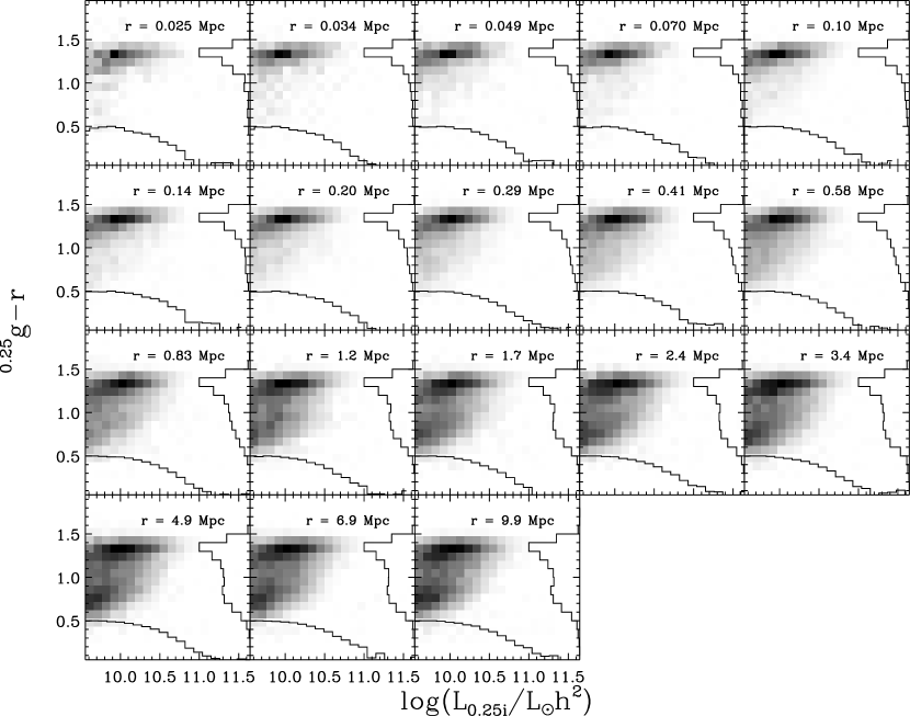
The density measured with this technique may be tabulated in various ways, typically as a function of projected radial separation . We tabulate in a cube that represents bins of separation , luminosity , and color . This choice facilitates the study of the radial dependence of the luminosity function and the color–density relation. We make measurements for objects in the ranges Mpc (in 18 bins), (in 20 bins) and log (in 20 bins), where and were K-corrected to the median redshift of the cluster sample, . Note that the smallest separation that we use is 20 kpc, interior to which the light is dominated by the BCG. We retain information about the BCG of each cluster separately. An example of the resulting distributions is shown in Figure 1: each panel shows the joint color–luminosity distribution in the richness bin 12 17 for a different radial range, the mean of which is indicated in the legend of each panel. We save the cubes of luminosity density and number density data for every cluster, then bin the clusters into samples based on cluster observables. We evaluate the uncertainties for our results using jackknife estimation from dividing the survey area into 12 roughly contiguous, roughly equal area sections.
For each bin in richness, the projected radial profiles as a function of luminosity and color are inverted using a standard Abel type integral to recover the three-dimensional profiles. The inversion relates the derivative of , the projected number density profile, to , the 3D density profile, as
| (7) |
where is the excess density over the mean random background . Inherent in this inversion is the assumption that is the line-of-sight projection of a spherically symmetric . In an isotropic universe this assumption is valid as long as cluster selection does not preferentially find systems oriented in a particular direction with respect to the observer.
We apply the nonparametric method of Johnston et al. (2007a) to deproject the number density profiles. Because the maximum separation we use is 10 Mpc, not infinity, we cannot constrain the 3D density at the outermost point, and the second to last point, at Mpc, must be corrected. With a power law extrapolation of the profile, the correction is 5% upward for that point. Deprojection is necessary to accurately recover the the red fraction and luminosity functions. Failure to properly deproject will result in artificially high faint-end LF slopes and artificially low red fractions (Valotto et al., 2001; Barkhouse et al., 2007). After deprojecting, we translate the bins of physical radial separation into bins of using the measured - relationship (see § 3.5). To make measurements within the same bins of for clusters of different richness, we use power-law interpolation between the fixed values tabulated in the data cube.
We construct the LF of clusters in a given richness range in the following manner. For each richness value, for a given bin in luminosity, we calculate the excess number density of galaxies in the desired color and range. For the LF of a broader richness bin, we average the LFs of all clusters in that richness range. To measure the red fraction for clusters in a given richness range, we follow an analogous procedure: we find the number of red and all galaxies in the desired luminosity and range for each cluster richness, then take the average over all clusters within the broader richness bin. The number of red galaxies divided by the total number of galaxies (within the luminosity and limits) is the red fraction, . To measure the total luminosity of galaxies in a given , color, luminosity and richness range, we again follow the same procedure, but using the tabulated values of luminosity density, rather than number density.
These measurements allow investigation of the distribution of excess-over-random galaxies around the BCGs used as MaxBCG centers. If a significant fraction of BCGs are miscentered relative to the density peak of the dark matter halos (whether because the true BCG does not lie at the deepest part of the potential well or because the wrong galaxy was identified as the BCG during cluster detection), the resulting weak lensing profiles can be affected (Johnston et al., 2007a), as should the light profiles. In this work we make no miscentering correction, but remind the reader that we measure the distribution of galaxies around BCGs, not halo mass peaks.
3.2. Random Catalogs
To correct for the contribution of galaxies along the lines of sight to clusters, we generate a set of 15 million random points. These points are used in the , and terms from the estimator described in equation 2. The random positions are distributed uniformly over the survey area using the window function described in § 3.3. The redshifts used for random points must statistically match that of each cluster sample in order for the background subtraction to be accurate. To achieve the proper distribution, the random primaries were generated with constant comoving density. For a given subsample of clusters we re-weight the random primaries so that the weighted redshift distribution matches that of each cluster subsample when binned with = 0.01.
3.3. Survey Geometry
We characterize the survey geometry using the SDSSPix code444http://lahmu.phyast.pitt.edu/scranton/SDSSPix/. This code represents the survey using nearly equal area pixels, including edges and holes from missing fields and “bad” areas near bright stars. We remove areas with extinction greater than 0.2 magnitudes in the dust maps of Schlegel et al. (1998). This window function was used in the cluster finding and in defining the galaxy catalog for the cross-correlations. By including objects only from within the window, and generating random catalogs in the same regions, we control and correct for edges and holes in the observed counts as described in § 3.1. The resulting area examined is 7398.23 deg2.
The denominator terms and in equation 2 correct for the survey edges and holes by measuring the actual area searched. An example is shown in Figure 2, generated for one richness bin. This quantity is expressed as the mean fractional area searched relative to the area in the bin. For small separations, edges and holes make little difference, so the fractional area searched is close to unity, but on larger scales edges become important.
On very small scales the area probed in each bin is relatively small and the correction factor is not well constrained. However, we know that the area correction factor must be close to unity, a fact that is clear from visual inspection. To smooth the result, we fit a fifth order polynomial, constrained to be unity on small scales, to the fractional area as a function of the logarithmic separation. Due to the weighting, this approach results in a curve that approaches unity smoothly on small scales, yet matches intermediate separation points exactly. Points on larger scales are well-constrained and do not need smoothing.
3.4. K-corrections
We calculated K-corrections using the template code kcorrect from Blanton et al. (2003a). This code is accurate but too slow to calculate the K-corrections for the over pairs found in the cross-correlations. To make the computation tractable, we computed K-corrections on a grid of colors in advance using galaxies from the SDSS Main sample as representative of all galaxy types. We computed the K-corrections for these galaxies on a grid of redshifts between 0 and 0.3, the largest redshift considered for clusters in this study. The mean K-correction on a 21x21x80 grid of observed , and was saved. We interpolated in this cube when calculating the K-correction for a given galaxy. This interpolation makes the calculation computationally feasible for this study, but is still the bottleneck.
To minimize uncertainties in the K-correction, we K-correct to the median redshift of the cluster sample, . All reported magnitudes are adjusted to this redshift, and are noted as e.g., . Blanton et al. (2003b) give a complete discussion of this bandpass shifting procedure.
3.5. r200 and M200
There has been much recent work to quantify the mass–observable relation for stacked samples of the maxBCG clusters, using mass estimates from cluster abundance (Rozo et al., 2007b), velocity dispersion (Becker et al., 2007), weak lensing (Sheldon et al., 2007a; Johnston et al., 2007b), and X-ray measurements (Rykoff et al., 2007). These various methods all result in a consistent mass–richness scaling; a detailed comparison of the different mass estimators is in progress (Rozo et al. in preparation). These measurements also yield estimates of cluster size.
To compare equivalent regions of clusters of various masses and thus various sizes, we scale all physical radii to , where is the threshold radius interior to which the mean mass density of a cluster is 200 times the critical mass density of the Universe. The weak lensing-measured of Johnston et al. (2007b) yields a size-richness relationship of
| (8) |
which we use here. As we have measured 3D profiles around all clusters out to 8 Mpc, we can construct 3D radial profiles out to 5 for even the most massive systems in our catalog.

For comparison, we also derive using the approach presented in Hansen et al. (2005) for estimating as a function of using the space density of galaxies in clusters. In that work, the radial space density profile of cluster-correlated galaxies brighter than a luminosity threshold was compared with the global mean space density as determined from the global SDSS luminosity function (Blanton et al., 2003b), evolved to , integrated to the same luminosity threshold. The radius interior to which the mean space density of cluster galaxies reached 200/ times the global mean density of galaxies was taken as . If galaxies were completely unbiased with respect to dark matter on all scales, measured with galaxies should exactly match measured from the true mass distribution. The characteristic cluster-associated galaxy used has a luminosity of slightly sub-. On average in the Universe, a galaxy with this luminosity has a bias of close to unity. As our sample is specifically chosen to be galaxies associated with clusters, however, and clusters do not present the same environment as the cosmological average, we cannot necessarily expect that the typical cluster galaxy thus also has bias close to one. Nonetheless, we show below that using these galaxies as a tracer of the total matter distribution does result in a reasonable approximation of , a finding also noted by Gonzalez et al. (2007).
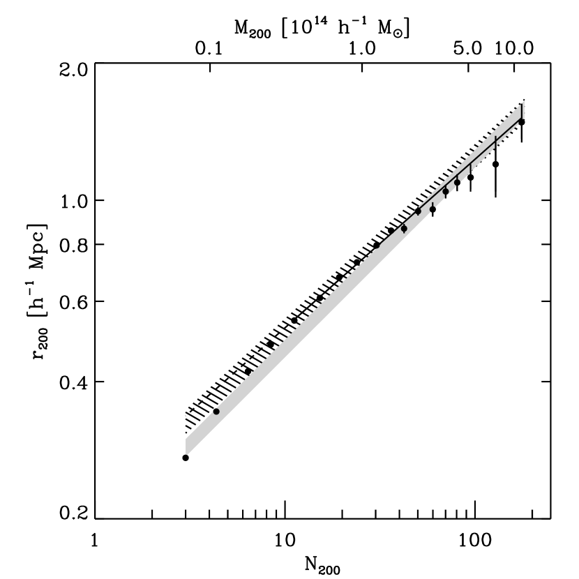
Using the galaxy distribution-based method with the current data set, and comparing to the field sample, we find for that Mpc . Figure 3 shows as estimated from the galaxy distribution (points with error bars), the relationship from the velocity dispersion-based mass estimate (hashed region), and the lensing estimate (shaded region). The width of the hashed region corresponds to a 18% uncertainty in the mean mass–observable relationship from Becker et al. (2007); the width of the shaded region corresponds to a 13% uncertainty in mass as reported for the lensing analysis in Johnston et al. (2007b). The best fitting power law for 10 for the galaxy-based measurement is plotted as the solid line, with a dashed line extending the trend to lower richness. The derived from the galaxy distribution is remarkably consistent with these other observations. The slight discrepancy in scaling gives hints about the way that galaxies populate halos of dark matter, but further investigation of this interesting problem is beyond the intended scope of this work.
The measurement of also enables an estimate of cluster mass, . For the present work, we present our results as a function of the direct observable, , but use the – relationship from the weak lensing analysis to translate this observable into a mass estimate. The mass is calculated from via
| (9) |
where is the critical density at epoch , and the Hubble parameter is given by for a flat LCDM Universe. For the choices of and used in Johnston et al. (2007b), the – conversion is . We therefore adopt
| (10) |
the best-fit value from Johnston et al. (2007b). We note that these values are measured in the lensing data including the effects of miscentering, and so should reflect the underlying halo mass, rather than the mass correlated with cluster centers.
3.6. Testing with Simulation Data
To check that our methods of background correction and deprojection are reliable, we compare the SDSS data to results from a mock catalog from an N-body simulation populated with galaxies using the ADDGALS method of of Wechsler et al. (2007). This catalog is derived from the N-body Hubble Volume light-cone simulation (Evrard et al., 2002). Particles in the simulation are assigned luminosities to match the luminosity-dependent two-point correlation function measured in the SDSS by Zehavi et al. (2005) and the global SDSS luminosity function (Blanton et al., 2003b). Colors are assigned depending on local environment as defined by the distance to the 5th nearest neighbor, matching the photometric properties of SDSS galaxies with similar luminosities and local densities. The luminosity limit of the mock catalog is L 0.4, matched to the luminosity threshold used for identifying MaxBCG clusters. This mock catalog successfully reproduces the width, location and evolution of the red ridgeline, making it ideal for testing and understanding the selection function of the MaxBCG algorithm. A detailed characterization of the MaxBCG selection function based on this catalog has been undertaken by Koester et al. (2007b) and Rozo et al. (2007a).
We use this simulation to test the algorithms presented for quantifying the galaxy population. We run the MaxBCG cluster finder on the mock catalog, then implement the same background-correction algorithm used on the SDSS data to characterize the galaxy population statistically associated the MaxBCG-identified cluster centers. In order to test the algorithms, we compare the properties of galaxies located in three dimensions around MaxBCG-identified cluster centers with the statistical distribution of galaxies determined by the background-correction algorithm run on the mock. The mass limit for resolved halos in the simulation, , allows a close to complete sample for a richness of , so we focus on results above that range.
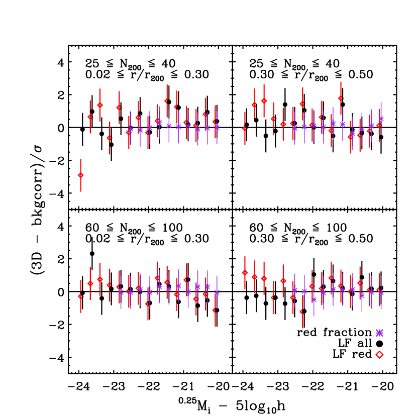
We find that the background-correction algorithm does well at reproducing the underlying distribution. For example, Figure 4 demonstrates that the difference between the underlying 3D values and the background-corrected values for several statistics are typically within . Shown is the comparison between the luminosity functions of all galaxies (filled circles) and red galaxies (diamonds). Also shown is the comparison of red fraction values (asterisks). In all cases the difference is expressed in units of the uncertainty . The left column is for galaxies within , while the right column is for galaxies in the range ; the top panels are a low richness bin (25 40) and the bottom panels are a high richness bin (60 100). For magnitudes brighter than - 5log -23, there are no galaxies found, so the red fraction is not calculated.
4. Results
Our primary results comprise the luminosity and color distributions for cluster galaxies as a function of cluster richness, cluster-centric distance, and redshift. We examine BCG and satellite galaxies separately, motivated by the observational and theoretical reasons previously discussed. As an example of BCG-satellite differences, Figure 5 shows the luminosity function for all galaxies within of cluster centers for four different bins of cluster richness. The luminosity functions of the satellites (filled circles) and BCGs (open diamonds) are shown separately; the total LF is given by the black line (with error bars omitted for clarity). Examination of the reveals that the satellite LF is statistically well described by a Schechter function, but this behavior is not the case when the BCG is included. The BCG-only LF is well-fit by a single Gaussian. In lower richness clusters, the BCGs dominate the total light but are systematically fainter and have larger luminosity variance than BCGs in larger systems. These differences illustrate one way in which BCGs tend to be distinct from satellites.
We begin by presenting results describing the satellite population, then turn to the BCGs. In § 4.1, we examine the luminosities and colors of satellites. Specifically, we measure the luminosity function of satellies within as a function of cluster richness; this measurement is closely related to the conditional luminosity function that is parametrized as a function of mass. We also investigate the CLF of red and blue satellites separately, and show the radial trend of the LF for all, red, and blue satellites. In addition, we measure the red fraction of satellites and investigate its dependence on several cluster properties. In §4.2 we explore the BCG population and quantify the relationships of BCG luminosity to total cluster mass and to satellite total and characteristic luminosity.
4.1. Satellite Cluster Galaxies
In this section we measure the conditional luminosity function and its dependence on galaxy color and cluster-centric distance. We also study how the red fraction depends on redshift, cluster mass, cluster-centric distance, and galaxy luminosity.
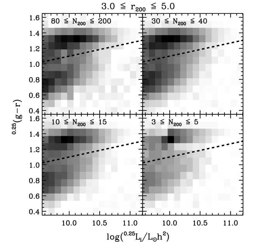
To split the galaxies into red and blue subsamples, we make a cut in color–luminosity space:
| (11) |
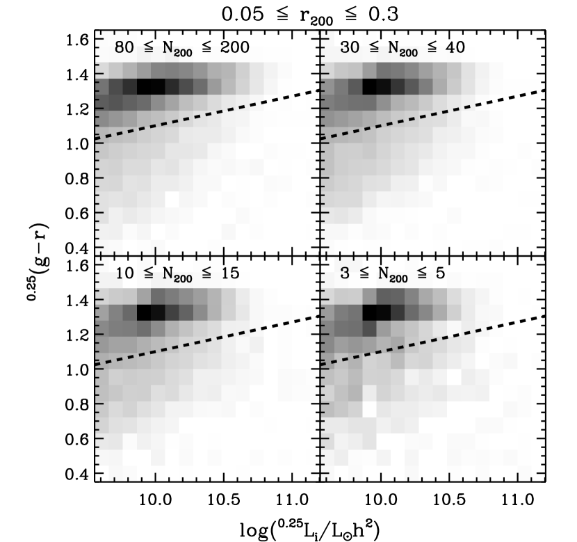
Because of the strong bimodality in the population, our results do not depend sensitively on the exact placement of the red–blue boundary. Figure 6 shows the bivariate distribution of color and luminosity for four example richness bins and two radial ranges: ; ; ; and (left set of 4 panels); (right set of four panels) respectively. The red sequence exists at all richnesses. Even at large radii, there is an excess over random of galaxies associated with clusters, and many of them are blue. The dashed line in the figure shows our adopted cut between red and blue galaxies.
4.1.1 Conditional Luminosity Functions
We start by investigating the dependence of total, as well as red and blue split, luminosity functions on cluster richness and cluster-centric distance. We use bins defined by sharp cuts in richness; due to scatter in the mass–observable relationship, each bin therefore contains clusters from a non-sharply defined mass range. Note that these observationally-defined conditional luminosity functions, which depend on both richness and cluster-centric distance, are related to but differ somewhat in definition from the traditional definition of the CLF as a function of cluster mass where the binning is done in specific mass ranges (as in, e.g., Yang et al., 2003).
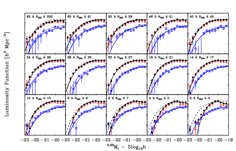
Figure 7 shows the luminosity function of satellite galaxies within for different bins of cluster richness. These LFs are shown for all satellites (filled circles) and for the blue and red subsamples separately (open squares and open diamonds respectively). The shape of the overall satellite LF is only weakly dependent on for the top two rows, representing higher clusters. These are the systems that have been well studied and are known to be quite complete and pure. For , sub- and super- satellites are both found with lower density than in more massive systems, but the incidence of galaxies is about the same as in the higher-mass objects. With the split into red and blue subsamples, we see that change in the faint end of the overall LF is driven by the changing ratio of red and blue galaxies. We investigate the changing fraction of red galaxies as a function of galaxy luminosity and cluster mass further in § 4.1.2.
We fit the above LFs with Schechter (1976) functions,
| (12) | |||||
using the Levenburg-Marquardt minimization procedure. The solid black lines in Figure 7 show the best-fitting Schechter function for the total satellite LF in each richness bin. The satellite LF is well fit by a Schechter function except for in the very lowest richness bin. For reference, the best-fit Schechter function to the mean satellite LF for clusters with is repeated in all panels as a dashed line. We also fit a Schechter function to the LF of the blue and red galaxy populations. For blue satellites, in the cases where the fit is well constrained, we find the faint end slope to be . In some cases the blue data do not permit a strong constraint on the faint-end slope. We therefore fit the blue LFs with a faint-end slope fixed to be 1.0. These Schechter functions for blue satellites is shown in each panel as the solid blue line, and for comparison, the best fit for the mean blue satellite LF of clusters with is repeated in all panels as a dot–dashed line. The fits for the red satellites are omitted for the sake of clarity.
| Parameter | Units | Vs. | ||
|---|---|---|---|---|
| 0.25….. | 0.8 0.1 | 0.15 0.04 | ||
| 1.29 0.02 | 0.12 0.03 | |||
| ………… | -0.28 0.06 | 0.25 0.07 | ||
| -0.63 0.02 | 0.20 0.05 | |||
| ………. | Mpc-3 | 8 1 | -0.20 0.04 | |
| Mpc-3 | 4.3 0.1 | -0.16 0.03 |
Note. —
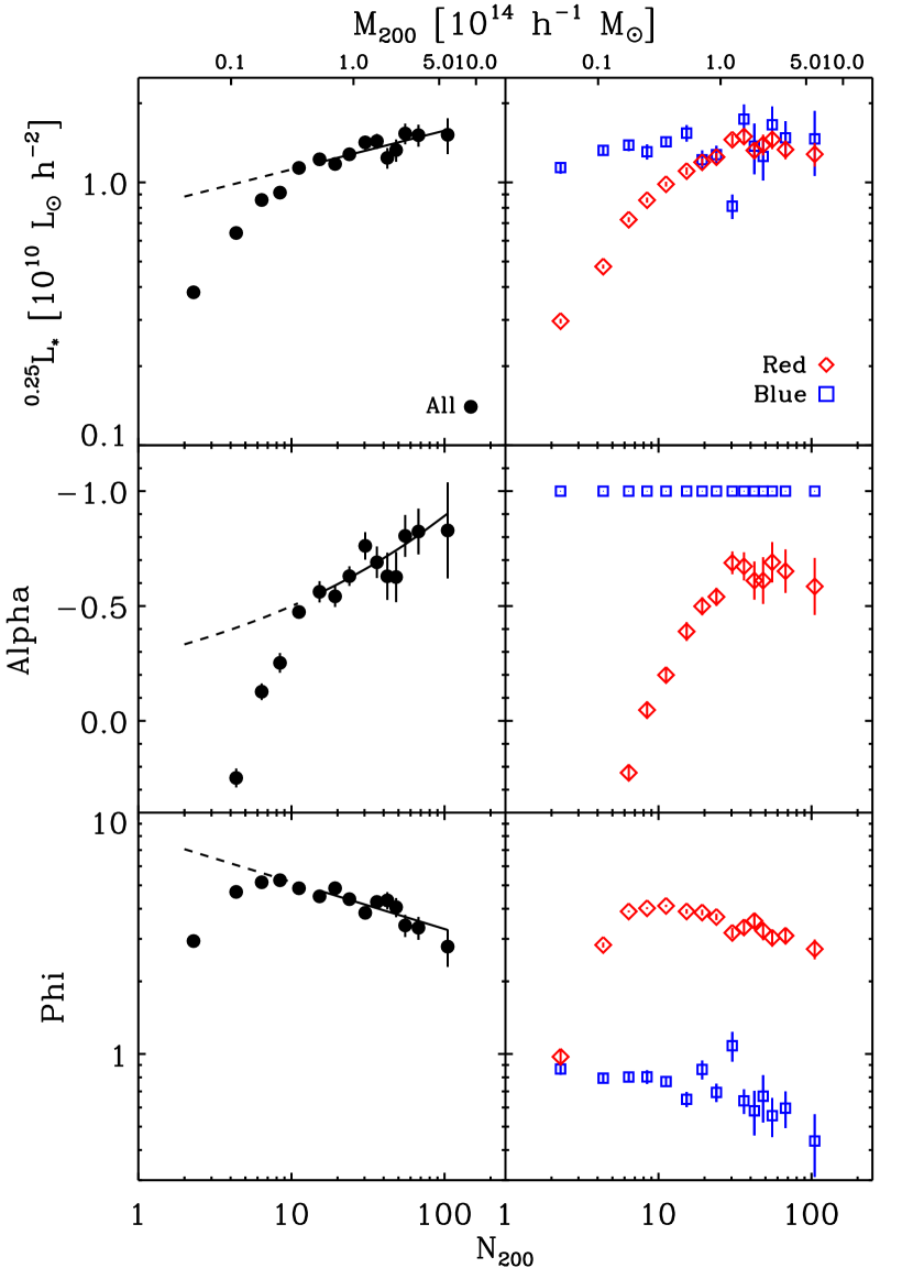
The parameters of these best-fitting Schechter functions are shown in Figure 8 as a function of . For systems with 10, 0.25 for all satellites is a weak function of mass, and is roughly . For blue galaxies in clusters of any richness, 0.25 is consistent with ; red galaxies have consistent with this value only for 30 (), while lower mass systems have red satellites with a fainter characteristic luminosity. The faint end slope, , scales with mass for all and red satellites, with a steeper faint end slope for more massive clusters. For blue galaxies, we have fixed the value of , but by inspection of Figure 7 it is seen that changes little over the whole richness range of the catalog. The normalization of the LF, , decreases with mass for all, red, and blue galaxies. For each of , and , we fit the trend of the parameter as a function of richness for . The fits are shown on the Figure, with a solid line where the fit was performed and a dashed line extending the relationship to lower richness. The parameters of these fits are listed in Table 1.
These CLF results show the weak dependence of the LF parameters on cluster mass, and are in reasonable agreement with other recent modeling and observational results. The relationship between characteristic satellite luminosity and cluster richness was recently discussed by Skibba et al. (2007). They explored the predictions of Skibba et al. (2006) that, for halos with mass greater than , their Halo Occupation Distribution (HOD) models predict that the mean luminosity of non-central galaxies should be nearly independent of mass and that the shape of the LF is approximately independent of mass. Skibba et al. (2007) showed that the mean non-central galaxy luminosity is indeed only very weakly dependent on cluster richness (as quantified by the number of galaxies with ) in the group catalogs of Yang et al. (2005) and Berlind et al. (2006). The catalogs used in Skibba et al. (2007) just barely overlap in mass with the lower mass end of our sample. Our findings for are in agreement with the group-scale results, and show that the HOD prediction continues to hold for greater mass systems as well. The results of CLF modeling discussed in Cooray (2005) and Cooray (2006), based on constraints from the two-point correlation function, also qualitative agree with this the behavior of as a function of cluster mass.
The dependence of the faint end slope on has also been discussed elsewhere; Cooray (2005, 2006) also found a steeper faint end slope for more massive systems, and a changing faint end slope was incorporated into the CLF models of van den Bosch et al. (2005) in a similar way to fit the observed trends in 2dFGRS data. The trend for the faint end falling off more rapidly in less massive systems is qualitatively similar to the trend seen in RCS-1 data (Gilbank et al., 2007), although more work is required to make a detailed comparison with this higher-redshift, and very differently selected, sample. We note that the magnitude limit of our data is a relatively bright - 5log , so we cannot comment on the faint end turn-up seen in deeper studies (Yagi et al., 2002; Popesso et al., 2006; Barkhouse et al., 2007). Our results for all, red, and blue satellites are in good agreement with these deeper results in the magnitude range where we overlap.
The somewhat counter-intuitive trend of decreasing in more massive systems reflects the correlation between (M/L)200, the mass-to-light ratio measured at , and cluster mass. The (M/L)200– relationship is both expected theoretically in some models (e.g., Tinker et al., 2005; van den Bosch et al., 2007, and references therein) and directly observed (Sheldon et al., 2007b). By definition, the mass density within is the same for clusters of all masses. Since (M/L)200 increases as a function of cluster mass, the luminosity density must be decreasing with mass. As the typical galaxy luminosity increases with mass, the mean number density of galaxies within must decrease with mass.
In Hansen et al. (2005) we explored the LFs of galaxies in clusters as a function of richness, and it was not clear that all satellite LFs within were well described by a Schechter function, especially for the low-richness systems. However, the cluster finder used in that previous work used a fixed 1 Mpc aperture for estimating richness, resulting in much greater scatter in the mass–richness relation than in the present version of the cluster-finding algorithm, thereby mixing together clusters of much different mass into the same bin of richness. In addition, as we will show, the LF normalization changes dramatically as a function of , so a fixed aperture will mix populations from different fractional sections of clusters and thus further confuse the analysis. While any catalog will have noise and impurities, the current cluster catalog, which uses and improved richness measure, should be less affected by this issue.
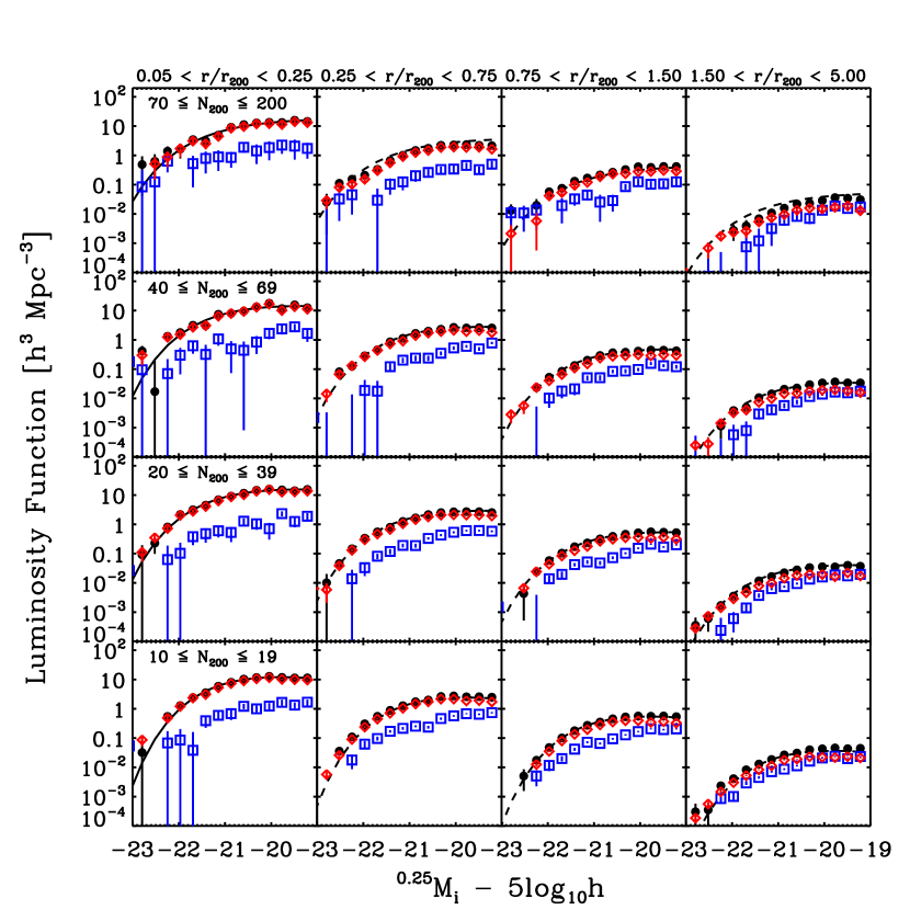
In addition to the LF within , we also investigate the radial dependence of the luminosity function for all galaxies and for red and blue galaxies separately in several bins of cluster richness. These results are shown in Figure 9. Cluster richness decreases downward in the array of plots, and the radius range increases to the right. There are still galaxies correlated with the clusters centers at separations much larger than . While these galaxies are likely not bound to the clusters, they are statistically correlated with clusters and the amplitude of the luminosity function reflects the amplitude of the cluster-galaxy cross-correlation function.
The normalization of the LF decreases with cluster-centric distance, but the shape of the total satellite LF remains essentially unchanged for the magnitude range considered here. To illustrate this point, we have re-drawn the best-fit Schechter function for all satellites in the innermost radial bin (solid lines in left hand column) in the panels for other radial bins, but rescaled by (dashed lines in other columns). This rescaled LF is an excellent match to the measurements. For reference, we find that in the , and radial bins respectively, is typically 20%, 3%, and 0.3% of in the innermost bin.
Although the relative mix of luminosities is unchanged with radius, there is a strong change in the relative mix of colors. Red galaxies are much more dominant in the inner regions, and the decreasing contribution of red galaxies to the total LF at large radius is driven by changes in the faint end slope of the red LF. The shape of the blue galaxy luminosity function changes relatively little with radius, and at all radii the blue LFs show proportionately more faint galaxies than do the red or total LFs. The relative constancy of the bright end of the LF of all satellites as a function of radius is in agreement with the recent detailed examination of 57 low-redshift Abell clusters by Barkhouse et al. (2007), as is the finding that the LFs of red galaxies change more dramatically with radius than do the blue LFs.
These trends are discussed further in the context of the red fraction measurements below.
4.1.2 The Red Fraction & Other Color Statistics
From examination of the LFs, it is clear that the red fraction changes with a variety of parameters. In this section we examine the dependence of the red fraction on cluster richness, cluster redshift, cluster-centric distance, and satellite galaxy luminosity.
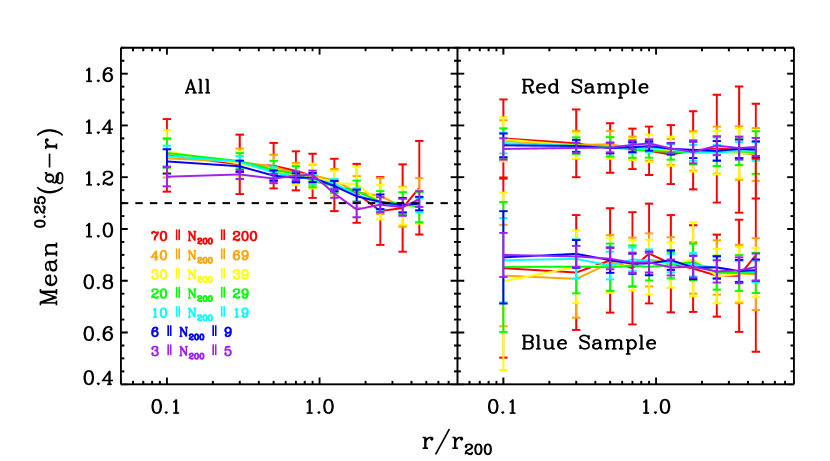
To assess whether changes in the galaxy population are primarily related to changes in the red fraction, we examine the typical color of satellites as a function of distance from the BCG. Figure 10 shows the (number weighted) mean color for satellite galaxies with - 5log , in bins of cluster-centric distance out to 5, and for several bins in cluster richness. The left panel shows the trend for all galaxies, while the right-hand panel shows the mean color for the red and blue samples of galaxies separately. The dashed line shows the estimated mean color of the universal average population. The overall mean satellite color is redder in the inner regions and trends bluer as a function of radius until , beyond which the mean color is consistent with the universal average value. The mean color is insensitive to cluster richness at any radius, with the exception of the very lowest richness bin in which the galaxies are typically bluer than in richer clusters. However, the right panel shows that the red and blue samples remain the same color regardless of cluster-centric distance or cluster richness, which implies that the overall shift in color is simply a change in the relative number of red and blue galaxies. This observation suggests either that there is some process that distributes red and blue galaxies differently with radius, or that the transition between the two populations happens fairly rapidly. Regardless of the mechanism, the color shift appears to be characterized well by the changing number of red galaxies, and we subsequently consider the red fraction, , as the primary statistic for quantifying the change in galaxy population.
We first measure the satellite red fraction within as a function of cluster richness and redshift. Figure 11 shows the fraction of red satellites brighter than - 5log and within as a function of cluster richness. The clusters are split into two bins of redshift: (filled circles, median ) and (open diamonds, median ). The red fraction increases significantly as a function of cluster mass in both redshift slices, but for lower redshift systems is systematically higher at all richnesses by 5%. There is a hint that flattens above . To parametrize the trend of red satellite fraction as a function of cluster richness and redshift, we adopt the functional form
| (13) |
We find that with
| (14) | |||
| (15) |
this form provides a reasonable description of the data; this relationship is shown as the solid lines in Figure 11. For , the catalog may be less than 90% complete and pure, and it is possible that as-yet-unquantified selection effects may influence the trend in this regime.
Here, we have made measurements within the aperture measured for the full cluster sample with the lensing data, relative to the critial density at . However, as the critical density scales with redshift, one can question whether we have biased our result by not using the taken relative to the critical density appropriate for the mean redshifts of the two subsamples. While the lensing analysis has not been done separately for the two redshift ranges, we can investigate the dependence of on redshift using the galaxy density estimate. We find that using the -appropriate threshhold for the high and low redshift samples results in values that are 8% and 1% different, respectively, from the value found for the whole sample. Using an adjusted aperture size, we measure red fractions that are 0.5% different for the higher redshift sample. The change in the low redshift sample is even smaller. This systematic offset is clearly not sufficient to explain the observed 5% difference in red fraction between the the two redshift bins.

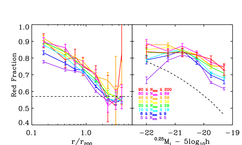
As seen from the behavior of the red and blue LFs, the red fraction has additional dependence on cluster-centric distance and satellite galaxy luminosity. In Figure 12 we examine both the radial and luminosity dependence of the red fraction. The left panel of Figure 12 shows for satelllies with - 5log for clusters in several bins in richness. Within , the red fraction decreases with radius. Beyond , flattens asymptotically, approaching the cosmological average (dashed line). The red fraction is essentially independent of cluster richness for systems, but is correlated with richness for .
The right panel of the Figure shows for satellites within as a function of absolute magnitude for multiple richness bins. For satellites brighter than , the red fraction is relatively independent of luminosity except for the lowest richness systems. For sub- galaxies, the red fraction steadily decreases toward fainter magnitudes, and the trend is stronger for lower systems. Except for the brightest galaxies in the very lowest-richness bin, is always greater than the universal average value (dashed line).
Broadly speaking, the fraction of red satellite galaxies increases with cluster mass, with galaxy luminosity, with time, and for decreasing cluster-centric distance. The dependence on cluster richness is coupled more strongly to satellite luminosity than to cluster-centric distance. The previous LF results showed that the faint ends of the red and blue satellites’ LFs change as a function of cluster-centric distance, although the bright ends remain essentially unchanged. In light of this observation, we conclude that it is the steadily changing mix of sub- galaxies as a function of distance from the cluster center that causes the trend of decreasing with cluster-centric distance.
These results are in general agreement with previous work, despite differences in sample definitions for both cluster selection and sample splitting. Several studies (Margoniner et al., 2001; Goto et al., 2003; Weinmann et al., 2006a; Poggianti et al., 2006; Martínez et al., 2006; Weinmann et al., 2006b; Gerke et al., 2007; Desai et al., 2007; Blanton & Berlind, 2007) have reported that the galaxy type fraction is a function of cluster mass. However, others (Balogh et al., 2004b; De Propris et al., 2004; Tanaka et al., 2004) found that the type fraction does not depend on cluster velocity dispersion, although Weinmann et al. (2006a) argues that this result may be due to the large scatter in relationship between velocity dispersion and mass. Furthermore, the flattening and “saturating” of the red fraction for the most massive systems appears to be a natural product of modeling (Berlind et al., 2003; Zheng et al., 2005). Some authors (De Propris et al., 2004; Weinmann et al., 2006a; Blanton & Berlind, 2007) have also found qualitatively similar behavior for the type fraction as a function of radius; however, this trend is very weak in both the Wilman et al. (2005) and Gerke et al. (2007) data, but there are large uncertainties in both of those data sets that could mask a correlation. The luminosity dependence of the galaxy type fraction is also similar to previous results (De Propris et al., 2004; Wilman et al., 2005; Weinmann et al., 2006a; Martínez et al., 2006; Gerke et al., 2007).
The redshift dependence of the galaxy type fraction has been discussed by many authors since Butcher & Oemler (1984). Overall, we find that the fraction of red galaxies increases by 5% during the 0.8 Gyr between our higher (median ) and lower (median ) redshift samples over the full mass range. This result is in quite good agreement with the results of the eponymous work, where an increase in the blue fraction by 0.25 in clusters to was observed (Butcher & Oemler, 1984). We also find agreement with Goto et al. (2003), who used a smaller catalog of clusters from the SDSS EDR. With the larger MaxBCG sample, however, we can see that this shift in red fraction happens in a similar manner for clusters of all richnesses. Direct comparison with higher redshift samples, such as the blue fraction of the DEEP2 groups measured by Gerke et al. (2007), is not straightforward because of the very different sample selection criteria used, but in future work we will undertake this comparison.
4.2. Luminosity of Brightest Cluster Galaxies
We now examine the Brightest Cluster Galaxies, focusing on their luminosities and how those luminosities compare to the total cluster luminosity and the characteristic satellite luminosity.
The top panel of Figure 13 shows the median luminosity of BCGs, , as a function of cluster richness. Systems with a greater number of satellites tend to host brighter BCGs. The error bars on the data points indicate the statistical uncertainty on the median BCG luminosity in each bin, determined from jackknife resampling; the dashed lines show the region within which 68% of the BCG luminosities lie. For , we parametrize the -richness trend with a power law, and find that the -band light from BCGs scales with cluster richness as
| (16) |
This fit is shown as a solid line Figure 13. Using our adopted mass–observable scaling, this relationship is
| (17) |
where we have defined . A scaling suggested by Vale & Ostriker (2006) for the -mass relation is
| (18) |
with , a = 29.78, b = 29.5, and k = 0.0255. This functional form is derived by fitting the relationship obtained by matching the galaxy luminosity function to the subhalo mass function, and is not currently physically motivated. Equation 18 also provides an acceptable fit to our data if we adopt , the mean galaxy luminosity in halos of in the -band. This relationship is shown on the Figure with the dot–dashed line.

The trend of increasing central galaxy luminosity with cluster richness has been noted in many previous observational studies (e.g., Sandage & Hardy, 1973; Sandage, 1976; Hoessel et al., 1980; Schneider et al., 1983). New large cluster samples with robust mass estimators have explored the scaling of BCG luminosity with cluster mass. Using a sample of 93 clusters with both X-ray and -band data, Lin & Mohr (2004) found that BCG light scales with mass as for clusters with , with significant scatter. Yang et al. (2005), using groups found in the 2dFGRS, found that in -band, for halos of M . Zheng et al. (2007), in their investigation of the luminosity-dependent projected two-point correlation function of DEEP2 and SDSS, also found that there is a correlation between halo mass and central galaxy luminosity. Using the Vale & Ostriker (2006) model, they see that provides a reaonable fit for the SDSS -band (with halo masses up to ) and is suitable for the DEEP2 -band data (with halo masses up to ). Using a different cluster catalog from the SDSS, Popesso et al. (2007) found for these 217 systems. Our results are in agreement with these findings within the uncertainties, but the size of the MaxBCG catalog, its well-understood selection function and its accurate mass estimator allow us to probe the BCG luminosity distribution in further detail.
At all richnesses, the distribution of is well-described by a Gaussian. The mean value is dependent on cluster richness as previously discussed. The width of the distribution, , is also a function of cluster richness. The bottom panel of Figure 13 shows as a function of richness, with error bars from jackknife resampling. There is an overall negative correlation between and , although for 35, is roughly consistent with a constant value of . This value is somewhat higher than the found by Zheng et al. (2007), but is consistent within the uncertainties. Our measurements are made as a function of cluster richness, and scatter in the mass–observable relation causes clusters over some range of masses to be assigned to each richness. Since depends on cluster mass, this scatter may result in larger observed values than in the intrinsic distribution of BCGs as a function of cluster mass. However, mass mixing acts only to increase the observed value, so our measurements represent at least a secure upper limit on the scatter in the – relationship. Future work with simulations is required to fully disentagle the intrinsic scatter from that introduced by the mass proxy.
The MaxBCG cluster finder includes priors on BCG color and luminosity (see § 2.2), and so we consider whether the resulting BCG luminosity distribution is being artificially constrained by these priors. In most cases, where BCG identification is unambiguous, only the narrow color priors inform BCG selection, so we do not expect a significant effect from the magnitude prior. Detailed examination of the effect of these priors on the selection function of MaxBCG is underway, but preliminary results indicate that the incidence of rich clusters with ambiguous BCGs is 25%, and does not have a significant effect on the scatter of rich systems. Here, we see that the width of the distribution of identified BCG -band absolute magnitudes is 0.5mag wider than the (mostly uninformative) magnitude prior, and that all BCGs are easily brighter than the nominal 0.4 limit. Thus, we take the recovered distributions as representative of the cluster population, but reserve a more detailed investigation for future work.
In addition to examining the correlation between BCG luminosity and cluster mass, we also measure the trend with mass of the ratios of BCG luminosity to the total cluster luminosity, , and BCG luminosity to the characteristic luminosity, , of the satellites. The top panel of Figure 14 shows / as a function of cluster richness. As expected from the example LFs of Figure 5, / decreases with cluster richness. For the most massive clusters (), the BCGs supply only of the cluster luminosity budget, but for intermediate systems the BCG makes up of the light. For the lowest richnesses the luminosity is completely dominated by the BCG.

Fitting a simple power law, we find that for clusters with , the BCG light fraction scales with cluster richness as
| (19) |
and with cluster mass as
| (20) |
This relationship is shown in the Figure with a solid line over the range where the fit was performed, and as a dashed line to extend the relation to lower richness.
The negative correlation between the BCG luminosity fraction and cluster mass is in good agreement with other results. The -band data presented by Lin & Mohr (2004) for their X-ray selected sample expresses qualitatively the same trend. For a different catalog of X-ray selected clusters, Popesso et al. (2007) measured the observed scaling between total optical luminosity and cluster mass and between BCG luminosity and cluster mass; the combination of these relationships yields a best fit scaling of / , consistent with our results. We are also in reasonable agreement with the low redshift (), -band model predictions of Tasitsiomi et al. (2007), who expect / 1/2 for massive systems, and who also predict that the normalization of this relationship may be sensitive to .
We also compare to the characteristic satellite luminosity . The value of is derived from fits to Schechter functions for satellites within and brighter than - 5log as in § 4.1.1. The bottom panel of Figure 14 shows that the ratio / depends strongly on . For clusters with , / increases with , but this trend reverses for very low richness systems. This behavior is not unexpected given the results of Figures 8 and 13: monotonically increases with , while is essentially flat for but correlated with richness for lower systems. We caution that the low richness ( ) systems should not be taken as representative of all low-mass systems, as the selection function imposed by the cluster finder (demanding only a few red galaxies in close proximity) may be important in this regime.
For , the ratio / as a function of cluster richness can be described by a power law:
| (21) |
and likewise as a function of mass:
| (22) |
This relationship is shown in the Figure with a solid line over the range in where the fit was performed and a dashed line to extrapolate the trend to lower richness.
5. Summary & Dicussion
In this study, we have examined the properties of cluster-associated galaxies, separating BCGs from satellites and focusing on trends in galaxy color and luminosity as a function of cluster richness, distance from cluster center, and redshift. We use clusters in the SDSS MaxBCG sample, the largest set of clusters identified to date. Employing photometric data alone, we apply cross-correlation background-correction techniques to characterize the cluster-associated galaxy population, within and brighter than - 5log , around 165,597 systems spanning more than two decades in mass in the redshift range .
Our principle results are as follows.
-
1.
The luminosity function of satellites within as a function of cluster mass for systems with mass greater than shows remarkable uniformity for - 5log . The characteristic satellite luminosity is only weakly dependent on cluster richness.
-
2.
The shape of the luminosity function of satellites brighter than - 5log does not change with cluster-centric radius. However, the color-separated luminosity functions of satellites as a function of and of show that the mix of sub- red and blue galaxies changes dramatically as a function of radius. In contrast, the relative number of red and blue galaxies at the bright end is roughly constant with radius.
-
3.
The average color of satellite galaxies is redder near cluster centers, but this trend is largely a reflection of the changing ratio of red to blue galaxies mentioned above. This effect is a very weak function of cluster mass over the range investigated here.
-
4.
The fraction of red galaxies increases with cluster mass over the full range explored, although only weakly for . This fraction decreases with cluster-centric distance until , decreases with luminosity for , and is constant for and .
-
5.
The fraction of cluster galaxies within that are red increases by 5% during the 0.8 Gyr between redshift to ; this change is roughly independent of mass over the range investigated.
-
6.
The luminosity of BCGs and the ratios of BCG luminosity to total cluster luminosity and to characteristic satellite luminosity are all correlated strongly with cluster mass, and we have quantified each of these scalings over the mass range to . The BCG luminosity has a Gaussian distribution at fixed cluster richness, with dispersion for clusters with .
While these results are in general agreement with previous observational work, due to the volume probed we are able to investigate a wider mass range, extending the statistics to higher mass than previous samples. We are also able to split the sample into finer bins for several variables than has previously been possible.
The MaxBCG selection function, which is well-understood for most of the richness range used here, is less well quantified for clusters with . This low richness set of clusters may be less complete and pure, which could result in the significant difference in LF shape as compared to higher systems, or contribute to the drop-off in for low richness systems. However, not all cluster galaxy properties change significantly at (e.g., /) and there is no break at a particular in either the mass–observable relationship (Johnston et al., 2007b) or mass-to-light ratios (Sheldon et al., 2007b) as measured by lensing. Interestingly, it is the quantities that most closely trace the total mass of the systems (i.e., , and the lensing signal) that are smoothly scaling over the full richness range, while quantities that are related to the mix of galaxies within clusters (i.e., the LF and ) are the ones that change more dramatically. We hypothesize that, at these low richnesses, MaxBCG is finding legitimate low-mass systems, but that the selection priors demanding the close proximity of only a few red galaxies result in finding only systems with the observed mix of galaxies and not necessarily all systems of this low mass. Further investigation using lower mass threshold mock catalogs is needed to understand in detail the selection of low-richness systems.
Our results can shed light both on the processes that build up the galaxy population in clusters and distinguish central galaxies from satellites, as well as the processes that are responsible for the galaxy transformation from blue to red. With respect to the former, the results presented here fit well within the basic picture of galaxy formation in CDM: that galaxy properties are likely linked to the formation history of a cluster’s dark matter halo and its substructures. Although detailed comparisons are beyond the scope of this work, our results qualitatively match both HOD constraints from clustering statistics as well as models based on matching the abundance of halos and subhalos to galaxies. The HOD framework provides a way to examine the galaxy population in both the observed Universe and in models of galaxy formation and evolution. Without needing to identify specific groups or clusters in the data, halo model interpretations of the statistics of luminosity-dependent galaxy clustering result in specific predictions for trends of both central and satellite galaxies as a function of halo mass that are in reasonable agreement with the findings presented here, especially for the relationship between central and satellite luminosities (e.g., Berlind et al., 2003; Skibba et al., 2007). Models which link the properties of galaxies directly to their halos and subhalos also agree broadly with several of the results presented here (e.g., Conroy et al., 2006; Vale & Ostriker, 2007). Detailed predictions for several cluster statistics from such a model will be presented in Tasitsiomi et al. (2007). Our results on scatter in the BCG luminosity at fixed cluster richness very likely provide an upper limit on scatter in central galaxy luminosity at fixed mass, as the scatter between halo mass and cluster richness should act to increase this scatter. The fact that this scatter is already fairly small provides further support for the tight coupling between halo mass and galaxy luminosity that is the basis of these models.
In addition to processes that cause physical changes to satellites resulting from interactions with the cluster gas, cluster potential, or other satellites, presumably some of the satellites are lost due to being accreted onto the BCG. In detail, this process likely results in the stellar component of the disrupted galaxy joining both the BCG and ICL (Conroy et al., 2007), but nonetheless should result in a BCG population closely linked to both halo mass and satellite population, as is observed. Indeed, / and / must be intimately related to the processes responsible for BCG growth. That BCGs get brighter as a function of cluster mass faster than do typical satellies may be further evidence that BCGs are different (in their merger history) than typical satellites.
Understanding the timescales and mechanisms for galaxies to transform from star-forming galaxies onto the red sequence is one of the primary current challenges for galaxy formation theories. There are several processes that can operate within clusters to shape the population of the cluster galaxies, such as ram pressure stripping, harassment and strangulation, that directly influence the galaxies’ gas content and thus their subsequent star formation (for a recent review, see De Lucia, 2006). Clearly many of the processes responsible for this transformation are related either to the mass of the host halo or how long the galaxies have been satellites. The relative strengths of various effects are still rather uncertain, however. What fraction of galaxies become red while they are central galaxies? Do the processes happen only for satellites in a certain mass range, or do they happen equally for all satellite galaxies? On what timescales do these processes operate? Our measurements of how the red fraction scales with cluster mass, radius and redshift will be instrumental in answering these questions.
We address a few of these issues here. Ram pressure stripping predicts that will be inversely correlated with cluster-centric distance, and larger for both brighter galaxies and more massive halos. However, our results indicate that is essentially independent of galaxy luminosity at fixed for galaxies brighter than and that the radial trend in is not any more pronounced in high systems. These results indicate that ram pressure stripping cannot be the dominant process at work to transform the galaxy population. The harassment scenario predicts that will be anticorrelated with cluster mass, as is observed; however, if this mechanism were dominant, then at fixed cluster mass would be expected to be larger for less luminous galaxies (Weinmann et al., 2006a), contradicting the observed trends. Strangulation, where star formation in infalling galaxies is halted because no further gas accretion is allowed, makes several predictions that are in good agreement with our observations. For example, the model presented by Diaferio et al. (2001) predicts: that the mean satellite color gets bluer as a function of cluster-centric distance until reaching a plateau at the field value around 2–3; that the mean satellite color depends on halo mass only for ; and that the incidence of blue galaxies in clusters increases at higher redshift. However, this model also predicts that both bulge- and disk-dominated satellies will get redder toward the central regions of clusters, a trend that we do not see in our red/blue sample split (or course, our color-separated subsamples are not directly comparable to their morphology-separated samples). Note that the predictions of such a model will in detail depend on its implementation. Our observation that the satellite red fraction changes in the same way with redshift regardless of cluster richness is significant evidence that the timescale of the physics responsible for quenching is the same in systems over the full mass range examined. The difference in cosmic time between the median redshifts of our two samples is approximately the dynamical timescale, over which we observe a 5% change in , and this observation should allow for useful constraints in studies on the details of quenching mechanisms.
A consensus is emerging from a variety of modeling efforts that star formation proceeds most efficiently in a mass range around , and is less efficient in more massive halos and for satellite galaxies. Simple models based on this type of assumption can produce many of the rough trends that we have seen here; for example, that the mean color of galaxies will not change significantly as a function of halo mass for the range of masses we investigate here (e.g., Diaferio et al., 2001), and that the galaxy type fraction should be a weak function of halo mass for (Berlind et al., 2003; Zheng et al., 2005; Cooray & Milosavljević, 2005). Furthermore, the general concept of galaxies falling in, quenching, and fading matches well with the observed radial trends of LF and red fraction. However, most of the detailed semi-analytic modeling efforts have had some trouble matching in detail observations of the color distribution of galaxies and how it changes with environment (see e.g., Coil et al., 2007). Unresolved issues include the rates at which star formation is triggered or shut off, and accordingly red galaxies tend to be overproduced. To understand in detail the physical mechanisms responsible for the quenching of star formation as clusters are assembled, further work is needed to accurately reproduce the observed trends in the cluster galaxy population. The present findings set a local-universe target for modeling results, and provide some guidance for the relative importance of some of the germane effects.
A substantial effort over the next decade will be devoted to large-scale, multi-band photometric surveys, including DES, Pan-STARRS, and LSST. Although the primary science driver of many of these projects is to investigate the nature of dark energy, the resulting data are likely to also provide strong constraints on the processes of galaxy evolution. The results presented here provide a low-redshift baseline against which current and future high-redshift samples may be compared. From a technical standpoint, these data are informative to next-generation cluster-finding techniques, and are useful input for creating the mock catalogs necessary for interpreting cluster surveys. Furthermore, the techniques presented here, which use photometric data alone, are directly applicable to these upcoming imaging surveys, and will thus enable detailed studies of the galaxy population at significantly higher redshifts without extensive spectroscopy.
References
- Abbott & The DES Collaboration (2005) Abbott, T. & The DES Collaboration. 2005, ArXiv Astrophysics e-prints, astro-ph/0510346
- Abell (1962) Abell, G. O. 1962, in IAU Symposium, Vol. 15, Problems of Extra-Galactic Research, ed. G. C. McVittie, 213
- Adelman-McCarthy et al. (2007) Adelman-McCarthy, J. K. et al. 2007, ArXiv e-prints, 707
- Allington-Smith et al. (1993) Allington-Smith, J. R., Ellis, R., Zirbel, E. L., & Oemler, A. J. 1993, ApJ, 404, 521
- Aragon-Salamanca et al. (1998) Aragon-Salamanca, A., Baugh, C. M., & Kauffmann, G. 1998, MNRAS, 297, 427
- Baldry et al. (2004) Baldry, I. K., Glazebrook, K., Brinkmann, J., Ivezić, Ž., Lupton, R. H., Nichol, R. C., & Szalay, A. S. 2004, ApJ, 600, 681
- Balogh et al. (2004a) Balogh, M. et al. 2004a, MNRAS, 348, 1355
- Balogh et al. (2004b) Balogh, M. L., Baldry, I. K., Nichol, R., Miller, C., Bower, R., & Glazebrook, K. 2004b, ApJ, 615, L101
- Balogh et al. (1997) Balogh, M. L., Morris, S. L., Yee, H. K. C., Carlberg, R. G., & Ellingson, E. 1997, ApJ, 488, L75
- Balogh et al. (2000) Balogh, M. L., Navarro, J. F., & Morris, S. L. 2000, ApJ, 540, 113
- Barkhouse et al. (2007) Barkhouse, W. A., Yee, H. K. C., & López-Cruz, O. 2007, ApJ, in press, arXiv:0709.0983 [astro-ph]
- Becker et al. (2007) Becker, M. R. et al. 2007, ApJ, in press, arXiv:0704.3614 [astro-ph]
- Bell et al. (2004) Bell, E. F. et al. 2004, ApJ, 608, 752
- Benítez et al. (2004) Benítez, N. et al. 2004, ApJS, 150, 1
- Berlind et al. (2003) Berlind, A. A. et al. 2003, ApJ, 593, 1
- Berlind et al. (2006) —. 2006, ApJS, 167, 1
- Bernardi et al. (2007) Bernardi, M., Hyde, J. B., Sheth, R. K., Miller, C. J., & Nichol, R. C. 2007, AJ, 133, 1741
- Bernstein et al. (2002) Bernstein, R. A., Freedman, W. L., & Madore, B. F. 2002, ApJ, 571, 56
- Blanton & Berlind (2007) Blanton, M. R. & Berlind, A. A. 2007, ApJ, 664, 791
- Blanton et al. (2005a) Blanton, M. R., Eisenstein, D., Hogg, D. W., Schlegel, D. J., & Brinkmann, J. 2005a, ApJ, 629, 143
- Blanton et al. (2003a) Blanton, M. R. et al. 2003a, AJ, 125, 2348
- Blanton et al. (2003b) —. 2003b, ApJ, 592, 819
- Blanton et al. (2005b) —. 2005b, AJ, 129, 2562
- Boylan-Kolchin et al. (2006) Boylan-Kolchin, M., Ma, C.-P., & Quataert, E. 2006, MNRAS, 369, 1081
- Brough et al. (2005) Brough, S., Collins, C. A., Burke, D. J., Lynam, P. D., & Mann, R. G. 2005, MNRAS, 364, 1354
- Brough et al. (2002) Brough, S., Collins, C. A., Burke, D. J., Mann, R. G., & Lynam, P. D. 2002, MNRAS, 329, L53
- Butcher & Oemler (1978) Butcher, H. & Oemler, Jr., A. 1978, ApJ, 226, 559
- Butcher & Oemler (1984) —. 1984, ApJ, 285, 426
- Byrd & Valtonen (1990) Byrd, G. & Valtonen, M. 1990, ApJ, 350, 89
- Christlein & Zabludoff (2005) Christlein, D. & Zabludoff, A. I. 2005, ApJ, 621, 201
- Coil et al. (2007) Coil, A. L. et al. 2007, ApJ, submitted, arXiv;0708.0004 [astro-ph]
- Conroy et al. (2006) Conroy, C., Wechsler, R. H., & Kravtsov, A. V. 2006, ApJ, 647, 201
- Conroy et al. (2007) —. 2007, ApJ, 668, 826
- Cooper et al. (2006) Cooper, M. C. et al. 2006, MNRAS, 370, 198
- Cooper et al. (2007) —. 2007, MNRAS, 376, 1445
- Cooray (2005) Cooray, A. 2005, MNRAS, 363, 337
- Cooray (2006) —. 2006, MNRAS, 365, 842
- Cooray & Milosavljević (2005) Cooray, A. & Milosavljević, M. 2005, ApJ, 627, L85
- Couch et al. (1998) Couch, W. J., Barger, A. J., Smail, I., Ellis, R. S., & Sharples, R. M. 1998, ApJ, 497, 188
- Croton et al. (2005) Croton, D. J. et al. 2005, MNRAS, 356, 1155
- Croton et al. (2006) —. 2006, MNRAS, 365, 11
- De Grandi et al. (2004) De Grandi, S., Ettori, S., Longhetti, M., & Molendi, S. 2004, A&A, 419, 7
- De Lucia (2006) De Lucia, G. 2006, ArXiv Astrophysics e-prints, astro-ph/0611350
- De Lucia & Blaizot (2007) De Lucia, G. & Blaizot, J. 2007, MNRAS, 375, 2
- De Propris et al. (2003) De Propris, R. et al. 2003, MNRAS, 342, 725
- De Propris et al. (2004) —. 2004, MNRAS, 351, 125
- Desai et al. (2007) Desai, V. et al. 2007, ApJ, 660, 1151
- Diaferio et al. (2001) Diaferio, A., Kauffmann, G., Balogh, M. L., White, S. D. M., Schade, D., & Ellingson, E. 2001, MNRAS, 323, 999
- Dressler (1980) Dressler, A. 1980, ApJ, 236, 351
- Dressler et al. (1997) Dressler, A. et al. 1997, ApJ, 490, 577
- Dubinski (1998) Dubinski, J. 1998, ApJ, 502, 141
- Edge & Stewart (1991) Edge, A. C. & Stewart, G. C. 1991, MNRAS, 252, 428
- Ellingson et al. (2001) Ellingson, E., Lin, H., Yee, H. K. C., & Carlberg, R. G. 2001, ApJ, 547, 609
- Evrard et al. (2002) Evrard, A. E. et al. 2002, ApJ, 573, 7
- Faber et al. (2007) Faber, S. M. et al. 2007, ApJ, 665, 265
- Fasano et al. (2000) Fasano, G., Poggianti, B. M., Couch, W. J., Bettoni, D., Kjærgaard, P., & Moles, M. 2000, ApJ, 542, 673
- Fukugita et al. (1996) Fukugita, M. et al. 1996, AJ, 111, 1748
- Gao et al. (2004) Gao, L., Loeb, A., Peebles, P. J. E., White, S. D. M., & Jenkins, A. 2004, ApJ, 614, 17
- Gerke et al. (2007) Gerke, B. F. et al. 2007, MNRAS, 376, 1425
- Gilbank et al. (2007) Gilbank, D. G., Yee, H. K. C., Ellingson, E., Gladders, M. D., Loh, Y. ., Barrientos, L. F., & Barkhouse, W. A. 2007, ApJ, in press, arXiv:0710.2351 [astro-ph]
- Gómez et al. (2003) Gómez, P. L. et al. 2003, ApJ, 584, 210
- Gonzalez et al. (2003) Gonzalez, A. H., Zabludoff, A. I., & Zaritsky, D. 2003, Ap&SS, 285, 67
- Gonzalez et al. (2005) —. 2005, ApJ, 618, 195
- Gonzalez et al. (2000) Gonzalez, A. H., Zabludoff, A. I., Zaritsky, D., & Dalcanton, J. J. 2000, ApJ, 536, 561
- Gonzalez et al. (2007) Gonzalez, A. H., Zaritsky, D., & Zabludoff, A. I. 2007, ApJ, 666, 147
- Goto et al. (2002) Goto, T. et al. 2002, PASJ, 54, 515
- Goto et al. (2003) —. 2003, PASJ, 55, 739
- Gunn & Gott (1972) Gunn, J. E. & Gott, J. R. I. 1972, ApJ, 176, 1
- Gunn et al. (1998) Gunn, J. E. et al. 1998, AJ, 116, 3040
- Gunn et al. (2006) —. 2006, AJ, 131, 2332
- Hansen et al. (2005) Hansen, S. M., McKay, T. A., Wechsler, R. H., Annis, J., Sheldon, E. S., & Kimball, A. 2005, ApJ, 633, 122
- Hoessel et al. (1980) Hoessel, J. G., Gunn, J. E., & Thuan, T. X. 1980, ApJ, 241, 486
- Hogg et al. (2001) Hogg, D. W., Finkbeiner, D. P., Schlegel, D. J., & Gunn, J. E. 2001, AJ, 122, 2129
- Hogg et al. (2004) Hogg, D. W. et al. 2004, ApJ, 601, L29
- Hubble (1926) Hubble, E. P. 1926, ApJ, 64, 321
- Ivezić et al. (2004) Ivezić, Ž. et al. 2004, Astronomische Nachrichten, 325, 583
- Johnston et al. (2007a) Johnston, D. E., Sheldon, E. S., Tasitsiomi, A., Frieman, J. A., Wechsler, R. H., & McKay, T. A. 2007a, ApJ, 656, 27
- Johnston et al. (2007b) Johnston, D. E. et al. 2007b, ApJ, submitted, arXiv:0709.1159 [astrop-ph]
- Kaiser et al. (2002) Kaiser, N. et al. 2002, in Presented at the Society of Photo-Optical Instrumentation Engineers (SPIE) Conference, Vol. 4836, Survey and Other Telescope Technologies and Discoveries. Edited by Tyson, J. Anthony; Wolff, Sidney. Proceedings of the SPIE, Volume 4836, pp. 154-164 (2002)., ed. J. A. Tyson & S. Wolff, 154–164
- Kauffmann et al. (2004) Kauffmann, G., White, S. D. M., Heckman, T. M., Ménard, B., Brinchmann, J., Charlot, S., Tremonti, C., & Brinkmann, J. 2004, MNRAS, 353, 713
- Kodama & Bower (2001) Kodama, T. & Bower, R. G. 2001, MNRAS, 321, 18
- Koester et al. (2007a) Koester, B. P. et al. 2007a, ApJ, 660, 239
- Koester et al. (2007b) —. 2007b, ApJ, 660, 221
- Larson et al. (1980) Larson, R. B., Tinsley, B. M., & Caldwell, C. N. 1980, ApJ, 237, 692
- Lin & Mohr (2004) Lin, Y.-T. & Mohr, J. J. 2004, ApJ, 617, 879
- Lin et al. (2004) Lin, Y.-T., Mohr, J. J., & Stanford, S. A. 2004, ApJ, 610, 745
- Loh & Strauss (2006) Loh, Y.-S. & Strauss, M. A. 2006, MNRAS, 366, 373
- Lubin et al. (2002) Lubin, L. M., Oke, J. B., & Postman, M. 2002, AJ, 124, 1905
- Lupton et al. (in preparation) Lupton, R. et al. in preparation
- Mandelbaum et al. (2006) Mandelbaum, R., Seljak, U., Kauffmann, G., Hirata, C. M., & Brinkmann, J. 2006, MNRAS, 368, 715
- Margoniner & de Carvalho (2000) Margoniner, V. E. & de Carvalho, R. R. 2000, AJ, 119, 1562
- Margoniner et al. (2001) Margoniner, V. E., de Carvalho, R. R., Gal, R. R., & Djorgovski, S. G. 2001, ApJ, 548, L143
- Martínez et al. (2006) Martínez, H. J., O’Mill, A. L., & Lambas, D. G. 2006, MNRAS, 372, 253
- Masjedi et al. (2006) Masjedi, M. et al. 2006, ApJ, 644, 54
- Matthews et al. (1964) Matthews, T. A., Morgan, W. W., & Schmidt, M. 1964, ApJ, 140, 35
- Menanteau et al. (2006) Menanteau, F., Ford, H. C., Motta, V., Benítez, N., Martel, A. R., Blakeslee, J. P., & Infante, L. 2006, AJ, 131, 208
- Moore et al. (1996) Moore, B., Katz, N., Lake, G., Dressler, A., & Oemler, A. 1996, Nature, 379, 613
- Oemler (1974) Oemler, A. J. 1974, ApJ, 194, 1
- Oemler et al. (1997) Oemler, A. J., Dressler, A., & Butcher, H. R. 1997, ApJ, 474, 561
- Ostriker & Tremaine (1975) Ostriker, J. P. & Tremaine, S. D. 1975, ApJ, 202, L113
- Pier et al. (2003) Pier, J. R. et al. 2003, AJ, 125, 1559
- Poggianti et al. (2006) Poggianti, B. M. et al. 2006, ApJ, 642, 188
- Popesso et al. (2006) Popesso, P., Biviano, A., Böhringer, H., & Romaniello, M. 2006, A&A, 445, 29
- Popesso et al. (2007) —. 2007, A&A, 464, 451
- Popesso et al. (2005) Popesso, P., Böhringer, H., Romaniello, M., & Voges, W. 2005, A&A, 433, 415
- Purcell et al. (2007) Purcell, C. W., Bullock, J. S., & Zentner, A. R. 2007, ApJ, 666, 20
- Rakos & Schombert (1995) Rakos, K. D. & Schombert, J. M. 1995, ApJ, 439, 47
- Robotham et al. (2006) Robotham, A., Wallace, C., Phillipps, S., & De Propris, R. 2006, ApJ, 652, 1077
- Rojas et al. (2005) Rojas, R. R., Vogeley, M. S., Hoyle, F., & Brinkmann, J. 2005, ApJ, 624, 571
- Rozo et al. (2007a) Rozo, E., Wechsler, R. H., Koester, B. P., Evrard, A. E., & McKay, T. A. 2007a, ApJ, submitted, arXiv:astro-ph/0703574
- Rozo et al. (2007b) Rozo, E. et al. 2007b, ApJ, submitted, arXiv:astro-ph/0703571
- Rykoff et al. (2007) Rykoff, E. S. et al. 2007, ApJ, submitted, arXiv:0709.1158 [astro-ph]
- Sandage (1976) Sandage, A. 1976, ApJ, 205, 6
- Sandage & Hardy (1973) Sandage, A. & Hardy, E. 1973, ApJ, 183, 743
- Schechter (1976) Schechter, P. 1976, ApJ, 203, 297
- Schlegel et al. (1998) Schlegel, D. J., Finkbeiner, D. P., & Davis, M. 1998, ApJ, 500, 525
- Schneider et al. (1983) Schneider, D. P., Gunn, J. E., & Hoessel, J. G. 1983, ApJ, 264, 337
- Schombert (1988) Schombert, J. M. 1988, ApJ, 328, 475
- Scranton et al. (2002) Scranton, R. et al. 2002, ApJ, 579, 48
- Sheldon et al. (2007a) Sheldon, E. S. et al. 2007a, ApJ, submitted, arXiv:0709.1153 [astro-ph]
- Sheldon et al. (2007b) —. 2007b, ApJ, submitted, arXiv:0709.1162 [astro-ph]
- Skibba et al. (2006) Skibba, R., Sheth, R. K., Connolly, A. J., & Scranton, R. 2006, MNRAS, 369, 68
- Skibba et al. (2007) Skibba, R. A., Sheth, R. K., & Martino, M. C. 2007, MNRAS, submitted, 707, arXiv:0707.3218 [astro-ph]
- Smail et al. (1995) Smail, I., Hogg, D. W., Yan, L., & Cohen, J. G. 1995, ApJ, 449, L105
- Smith et al. (2005) Smith, G. P., Treu, T., Ellis, R. S., Moran, S. M., & Dressler, A. 2005, ApJ, 620, 78
- Smith et al. (2002) Smith, J. A. et al. 2002, AJ, 123, 2121
- Strateva et al. (2001) Strateva, I. et al. 2001, AJ, 122, 1861
- Tanaka et al. (2004) Tanaka, M., Goto, T., Okamura, S., Shimasaku, K., & Brinkmann, J. 2004, AJ, 128, 2677
- Tasitsiomi et al. (2007) Tasitsiomi, A., Wechsler, R. H., Kravtsov, A. V., & Klypin, A. A. 2007, in preparation
- Tinker et al. (2005) Tinker, J. L., Weinberg, D. H., Zheng, Z., & Zehavi, I. 2005, ApJ, 631, 41
- Tonry (1987) Tonry, J. L. 1987, in IAU Symposium, Vol. 127, Structure and Dynamics of Elliptical Galaxies, ed. P. T. de Zeeuw, 89–96
- Toomre & Toomre (1972) Toomre, A. & Toomre, J. 1972, ApJ, 178, 623
- Tovmassian et al. (2004) Tovmassian, H. M., Plionis, M., & Andernach, H. 2004, ApJ, 617, L111
- Tremaine & Richstone (1977) Tremaine, S. D. & Richstone, D. O. 1977, ApJ, 212, 311
- Treu et al. (2003) Treu, T., Ellis, R. S., Kneib, J.-P., Dressler, A., Smail, I., Czoske, O., Oemler, A., & Natarajan, P. 2003, ApJ, 591, 53
- Tyson (2002) Tyson, J. A. 2002, in Presented at the Society of Photo-Optical Instrumentation Engineers (SPIE) Conference, Vol. 4836, Survey and Other Telescope Technologies and Discoveries. Edited by Tyson, J. Anthony; Wolff, Sidney. Proceedings of the SPIE, Volume 4836, pp. 10-20 (2002)., ed. J. A. Tyson & S. Wolff, 10–20
- Vale & Ostriker (2006) Vale, A. & Ostriker, J. P. 2006, MNRAS, 371, 1173
- Vale & Ostriker (2007) —. 2007, ArXiv Astrophysics e-prints, astro-ph/0701096
- Valotto et al. (2001) Valotto, C. A., Moore, B., & Lambas, D. G. 2001, ApJ, 546, 157
- van den Bosch et al. (2005) van den Bosch, F. C., Yang, X., Mo, H. J., & Norberg, P. 2005, MNRAS, 356, 1233
- van den Bosch et al. (2007) van den Bosch, F. C., Yang, X., Mo, H. J., Weinmann, S. M., Macciò, A. V., More, S., Cacciato, M., Skibba, R., & Kang, X. 2007, MNRAS, 376, 841
- van der Wel et al. (2007) van der Wel, A. et al. 2007, arXiv:0707.2787 [astro-ph]
- van Dokkum et al. (2000) van Dokkum, P. G., Franx, M., Fabricant, D., Illingworth, G. D., & Kelson, D. D. 2000, ApJ, 541, 95
- von der Linden et al. (2007) von der Linden, A., Best, P. N., Kauffmann, G., & White, S. D. M. 2007, MNRAS, 578
- Wechsler et al. (2007) Wechsler, R. et al. 2007, in preparation
- Weinmann et al. (2006a) Weinmann, S. M., van den Bosch, F. C., Yang, X., & Mo, H. J. 2006a, MNRAS, 366, 2
- Weinmann et al. (2006b) Weinmann, S. M., van den Bosch, F. C., Yang, X., Mo, H. J., Croton, D. J., & Moore, B. 2006b, MNRAS, 372, 1161
- Wilman et al. (2005) Wilman, D. J. et al. 2005, MNRAS, 358, 88
- Yagi et al. (2002) Yagi, M., Kashikawa, N., Sekiguchi, M., Doi, M., Yasuda, N., Shimasaku, K., & Okamura, S. 2002, AJ, 123, 87
- Yang et al. (2005) Yang, X., Mo, H. J., Jing, Y. P., & van den Bosch, F. C. 2005, MNRAS, 358, 217
- Yang et al. (2003) Yang, X., Mo, H. J., & van den Bosch, F. C. 2003, MNRAS, 339, 1057
- York et al. (2000) York, D. G. et al. 2000, AJ, 120, 1579
- Zabludoff & Mulchaey (1998) Zabludoff, A. I. & Mulchaey, J. S. 1998, ApJ, 496, 39
- Zehavi et al. (2005) Zehavi, I. et al. 2005, ApJ, 630, 1
- Zheng et al. (2007) Zheng, Z., Coil, A. L., & Zehavi, I. 2007, ApJ, 667, 760
- Zheng et al. (2005) Zheng, Z. et al. 2005, ApJ, 633, 791
- Zibetti et al. (2005) Zibetti, S., White, S. D. M., Schneider, D. P., & Brinkmann, J. 2005, MNRAS, 358, 949