Wave breaking and particle jets in intense inhomogeneous charged beams

Abstract

This work analyzes the dynamics of inhomogeneous, magnetically focused high-intensity beams of charged particles. While for homogeneous beams the whole system oscillates with a single frequency, any inhomogeneity leads to propagating transverse density waves which eventually result in a singular density build up, causing wave breaking and jet formation. The theory presented in this paper allows to analytically calculate the time at which the wave breaking takes place. It also gives a good estimate of the time necessary for the beam to relax into the final stationary state consisting of a cold core surrounded by a halo of highly energetic particles.

It is well known that magnetically focused beams of charged particles can relax from non-stationary into stationary flows with the associated particle evaporation reiser91 . This is the case for homogeneous beams with initially mismatched envelopes flowing along the magnetic symmetry axis of the focusing system. Gluckstern gluck94 showed that initial oscillations of mismatched beams induce formation of large scale resonant islands pak94 ; pak97 beyond the beam border: beam particles are captured by the resonant islands resulting in emittance growth and relaxation. A closely related question concerns the mechanism of beam relaxation and the associated emittance growth when the beam is not homogeneous. On general grounds of energy conservation one again concludes that beam relaxation takes place as the coherent fluctuations of beam inhomogeneities are converted into microscopic kinetic and field energy gluc70 ; reiser91 ; lund98 ; bern99 . However, unlike in the former case for which the specific resonant mechanism is well understood, for inhomogeneous systems a more detailed description of the processes involved must still be explored. This is the goal of the present letter.

The interest surrounding a better understanding of the dynamics of inhomogeneous beams is due to the fact that one can hardly design experimental devices capable of generating fully matched beams at the entrance of a transport system lund05 . While the azimuthal symmetry with respect to the beam axis is feasible in the case of focusing solenoidal magnetic fields, envelope matching — to avoid the radial oscillations — is significantly harder to achieve, while a perfect homogeneity is practically impossible.

Given all these facts, the purpose of the present work is to investigate the mechanisms leading to the decay of density inhomogeneities as the system relaxes into its final stationary state. We find that the relaxation comes about as a consequence of breaking of density waves followed by ejection of fast particle jets. Jets are formed by particles moving in-phase with the macroscopic density fluctuations. They draw their energy from the propagating wave fronts and convert it into microscopic kinetic energy. This process is very similar to the breaking of gravitational surface waves. The jet can then be compared to a broken crest of a gravitational wave surfing down the wave front. We stress that the wave breaking mechanism analyzed in this letter is very different from the Gluckstern resonances which were found to be the driving force behind the emittance growth in transversely oscillating homogeneous particle beams. For strongly inhomogeneous beams, we find that it is the wave breaking and jet production which are the primary mechanisms responsible for the beam relaxation.

We consider solenoidal focusing of space-charge dominated beams propagating along the transport axis, defined as the $z$ axis, of our reference frame. The beam is initially cold with vanishing emittance, and is azimuthally symmetric around the $z$ axis. Since the number of constituent particles is very large, the beam dynamics is governed by the azimuthally equation and collective effects are dominant. Prior to the appearance of density singularities, the original Vlasov formalism can be simplified to a cold fluid description for which Lagrangian coordinates are particularly appropriate. In these coordinates, the transverse radial position $r$ of a beam element is governed by ikegami97 ; davidson01 ; pak01 ; bru95

$$r^{\prime\prime}=-\kappa\,r+{Q(r_{0})\over r}.$$ (1)

The prime indicates derivative with respect to the longitudinal $z$ coordinate which for convenience we shall also refer to as “time”, and angular momentum in the Larmor frame is taken to be zero for each particle. The focusing factor is $\kappa\equiv(qB/2\gamma m\beta c^{2})^{2}$, where $B$ is the axial, constant, focusing magnetic field; $Q(r_{0})=KN(r_{0})/N_{t}$, is the measure of the charge contained between the origin at $r=0$ and the initial position $r(z=0)=r_{0}$, $N_{t}$ is the total number of beam particles per unit axial length, $N(r_{0})$ is the number of particles up to $r_{0}$, and $K=N_{t}q^{2}/\gamma^{3}m\beta^{2}c^{2}$ is the beam perveance. $q$ and $m$ denote the beam particle charge and mass, respectively; $\gamma=(1-\beta^{2})^{-1/2}$ is the relativistic factor where $\beta=v_{z}/c$ and $v_{z}$ is the constant axial beam velocity and $c$ is the speed of light. Note that $r_{0}$ is in fact the Lagrange coordinate of the fluid element morr98 which means that as long as the fluid description remains valid, the amount of charge seen by the fluid element inside the region $0<r\leq r(z)$ remains unaltered at $Q(r_{0})$, independent of time $z$. This is of fundamental importance since from the Gauss law this is the charge that exerts the force on the fluid element. In this letter we will consider the beams starting from a static initial condition, $r^{\prime}(0)=0$. The formal solution to the fluid dynamics Eq. (1) is $r=r(z,r_{0})$. This can be calculated explicitly using the Lindstedt-Poincaré perturbation theory. For small amplitude fluctuations around the stable equilibrium $r_{eq}(r_{0})=\sqrt{Q(r_{0})/\kappa}$ we obtain

$$r(r_{0},z)=r_{eq}\,\big{\{}1+A/r_{eq}\cos(\omega z)+(1/3)\>(A/r_{eq})^{2}\>\times$$ (2)

$$[2+\cos(\omega z)]\sin^{2}(\omega z/2)+{\cal O}[(A/r_{eq})^{3}]\big{\}}\;,$$ (3)

where $A(r_{0})=r_{0}-r_{eq}$ is the amplitude of oscillations, $\omega(r_{0})=\omega_{0}+\sqrt{\kappa}\,A^{2}/(6\sqrt{2}\,r_{eq}^{2})$ is the renormalized $r_{0}$-dependent frequency, and $\omega_{0}=\sqrt{2\kappa}$ is the unperturbed frequency. We stress that as long as the fluid picture applies, all the information about the temporal evolution of the beam is contained in Eq. (3). For example, the time evolution of the beam density can be obtained as follows. For a beam of initial cross sectional density $n_{0}(r)$, the amount of charge $\delta Q$ between two concentric circles of radii $r_{0}$ and $r_{0}+\delta r_{0}$ ($\delta r_{0}$ small) is $\delta Q=2\pi r_{0}\delta r_{0}(K/N_{t})n_{0}(r_{0})$. Since this charge is conserved, $\delta Q=2\pi r\delta r\>(K/N_{t})\,n\left(r\right)=2\pi r(\partial r/\partial r_{0})(K/N_{t})\,n(r)\delta r_{0}$, the transverse beam density at any future time $z$ is, therefore,

$$n(r)=n_{0}(r_{0})\,(r_{0}/r)\,\left(\partial r/\partial r_{0}\right)^{-1}\big{|}_{r_{0}=r_{0}(r,z)}.$$ (4)

For a given position $r$ and an axial coordinate $z$, the initial position $r_{0}$ of a beam element can be uniquely determined as the inverse function $r_{0}=r_{0}(r,z)$ of Eq. (3). This ceases to be the case if $\partial r/\partial r_{0}\rightarrow 0$ and $r_{0}(r,z)$ becomes multivalued. If this happens, the density will diverge and the fluid picture will break down. All these features, if present, would be indicative of a wave breaking phenomenon. Needless to say that presence of wave breaking in charged particle beams would be of considerable interest and practical importance. Breaking might be responsible for conversion of energy from macroscopic fluid modes into microscopic kinetic activity.

We start our analysis by considering the compressibility factor $\partial r/\partial r_{0}$, which can be obtained exactly by numerically integrating two nearby trajectories of Eq. (1) or approximately by differentiating Eq. (3). To be specific we write the initial cross sectional beam density at $z=0$ in a general parabolic form $n_{0}(r_{0})=\rho_{h}+\chi\rho_{i}(r_{0})$, where the inhomogeneity parameter $0\leq\chi\leq 1$, $\rho_{h}\equiv N_{t}/(\pi r_{b}^{2})$, and $\rho_{i}(r_{0})\equiv\rho_{h}(2r_{0}^{2}/r_{b}^{2}-1)$. $r_{b}$ is the beam radius. Note that the integral of the inhomogeneous contribution $\rho_{i}(r_{0})$ is zero. To suppress the effects arising from the pure envelope oscillations — Gluckstern resonances — we fix $r_{b}=\sqrt{K/\kappa}$, so that the beam radius is unaltered for as long as the fluid picture, Eq. (1), remains valid. We have also performed calculations for rms matched beams and find that they behave qualitatively the same way. Fig. 1 shows the typical time evolution of the compressibility $\partial r/\partial r_{0}$ obtained both numerically using Eq. (1) and analytically using (3). Since the amplitudes of oscillations of all fluid elements about the points of their equilibria are small, $|A/r_{eq}|\ll 1$, even for large values of $\chi$, the agreement between the numerical and the perturbative solution is found to be very good, see Fig. 1.

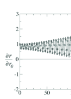
Figure 1: Time evolution of the compressibility factor $\partial r/\partial r_{0}$ for $\chi=0.6$ and $r_{0}=0.4r_{b}$. $\partial r/\partial r_{0}=0$ indicates singular density. Symbols represent the compressibility obtained from the numerical solution of Eq. (1), whereas the solid line is derived using the perturbative solution, Eq. (3). $z$ is measured in units of $\kappa^{-1/2}$. Position $r_{0}=0.4\,r_{b}$ is chosen because this is the approximate Lagrange coordinate at which density is first found to diverge for $\chi=0.6$.

The compressibility factor exhibits a fast oscillatory motion accompanied by a slow secular growth. This means that given enough time, the compressibility will always become zero for any finite value of $\chi$, resulting in a density divergence.

To further explore the significance of the diverging density, we have performed fully self-consistent N-particle simulations. For a system in which particles interact by an infinite range unscreened Coulomb potential, the time of collision diverges and the mean-field Vlasov description becomes exact brhe . Thus, in order to simulate the $N_{t}\rightarrow\infty$ limit — in which the thermalization time due to binary collisions is infinite — each particle can be taken to interact only with the mean-field produced by all the other particles. Taking advantage of the azimuthal beam symmetry and the Gauss law, a particle located at a position $r$ experiences a field generated by the particles within a circle of radius $r$ ikegami97 ; levin02 . We stress that in the $N_{t}\rightarrow\infty$ limit this is exact at any finite time scale. Within the simulation, the trajectory of each particle is, therefore, also governed by Eq. (1) — unlike the fluid elements, however, particles are allowed to bypass one another. This method avoids the thermalization effects associated with the binary collisions and significantly speeds up the simulations. It allows us to accurately simulate the collective effects dominant for all time scales when $N_{t}\rightarrow\infty$ even with a relatively small number of particles, $N_{t}\approx 10000$.

In Fig. 2 we display the particle phase-space $(r,v\equiv r^{\prime})$ for $\chi=0.6$. The first panel (a) shows the initial distribution at $z=0$ — all particles are still. In panel (b), after various propagating wave cycles, the system is about to build up an infinite density; velocity is still a single valued function of the space coordinate but a singularity (cusp) is forming. The third panel (c) shows the system at a time slightly larger than the first wave breaking time. Velocity ceases to be a single valued function of the space coordinate — while some of the particles go through the wave others do not. This latter class of particles is accelerated by the wave front and forms a thin azimuthally symmetric jet or finger seen in the figure. High energy jet particles can reach far outside the beam core and may be very detrimental to the beam transport. The process shown in panel (c) repeats itself many times, see panel (d), as the system evolves toward a final stationary state and the previously unoccupied extensions of the phase-space are gradually filled with particles whose velocities are considerably larger than velocities in the beam core. After some time a stationary state is reached in which the beam separates into a cold dense core and a hot and extended halo of ejected particles, panel (e). Time evolution of the emittance davidson01 $\varepsilon\equiv 2\,\sqrt{<r^{2}><v^{2}>-<r\,v>^{2}}$, where $<>$ denotes an average over particles, is shown in the last panel (f). At the wave breaking emittance suffers a sharp rise, followed by a rapid relaxation to the final stationary state in which large amplitude fluctuations subside. We note that beam relaxation is closely connected to phase-space filamentation. Phase-space filamentation takes place after particles are ejected from the beam core by surfing on the charge density waves. Once outside the core, particles experience the time dependent nonlinear forces and undergo all the complicated mixing dynamics with subsequent filamentation. This leads to final irreversible emittance growth. The directed emittance growth seen prior to relaxation is reversible.

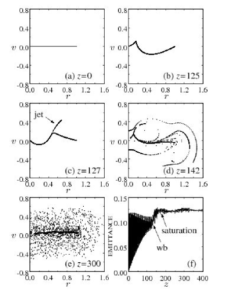
Figure 2: Time evolution in the phase-space $(r,v)$ for $\chi=0.6$. $r$ is measured in units of $(K/\kappa)^{1/2}$, $v$ in units of $K^{1/2}$, and $z$ in units of $\kappa^{-1/2}$: panel (a) – initial condition at $z=0$; panel (b) – after many wave cycles, but just before wave breaking; panel (c) – just after wave breaking, an azimuthal jet is expanding over the phase-space; panel (d) – while the first jet moves in the phase space new jets are being ejected; panel (e) – a phase portrait of a relaxed state; panel (f) – emittance growth leading to a final relaxation. Note that emittance saturates soon after the wave breaking (wb).

Since the beam radius $r_{b}$ is matched — envelope oscillations are small — the contribution of the Gluckstern resonant mechanism to the emittance growth and beam relaxation is, at most, marginal. The dominant mechanism is the singular build up of density followed by the wave breaking and jet production. The time of the first wave breaking depicted in the panel (c) of Fig. 2 agrees well with the time when the compressibility factor $\partial r/\partial r_{0}$ obtained from the Lagrange fluid equations goes to zero, Fig. 1. Our next goal is then to precisely calculate the instant at which the wave breaking takes place.

We first note that for an inhomogeneous density profile, each fluid element oscillates with a different frequency — rigid oscillations are possible only when the density profile across the beam cross section is homogeneous. Thus, nearby fluid elements will oscillate around their points of equilibria, slowly moving out-of-phase. This motion results in transverse density waves propagating across the beam. At some point, however, two nearby fluid elements will overlap one another leading to a singular build up of density. When this happens the fluid picture will lose its validity and will have to be replaced by the full kinetic description given in terms of the Vlasov equation. The wave breaking occurs when the separation between any two fluid elements vanishes, $r(r_{0}+\delta r_{0},z)-r(r_{0},z)\rightarrow 0$, for some value of $r_{0}$. This is precisely equivalent to our condition for the appearance of a singular density, $\partial r/\partial r_{0}\rightarrow 0$. Considering only the term linear in amplitude of Eq. (3), we see that $\delta r=\delta r_{eq}+\cos(\omega z)\delta A-Az\sin(\omega z)\delta\omega$. Neglecting the purely oscillatory term, as compared to the secular one, the time of breaking is found to be

$$z_{wb}\approx\min_{r_{0}}\left|{1\over 2\sqrt{Q}}{\partial Q/\partial r_{0}\over A\partial\omega/\partial r_{0}}\right|.$$ (5)

As expected, the breaking will always occur whenever $\partial\omega/\partial r_{0}\neq 0$. This is the case for all inhomogeneous particle beams. Unlike other systems in which one must have strong enough electric fields rosen02 , here any sort of inhomogeneity leads to the wave breaking — one just has to wait sufficiently long. As soon as the wave breaking takes place, particles with the same velocity as the density wave will be captured by the wave and surf down its front gaining kinetic energy (Fig. 2). Since at the wave breaking position $r_{0}/r_{b}<1$, minimization in Eq. (5) can be performed perturbatively in this parameter, yielding

$$z_{wb}=\left(3\over 2\kappa\right)^{1/2}\frac{\alpha^{3}\,\left(4\,{\sqrt{1-\chi}}+\chi-1\right)}{{\left({\sqrt{3}}-\alpha\right)}^{2}\,\left({\sqrt{1-\chi}}+\chi-1\right)},$$ (6)

where $\alpha\equiv{(1+2\,{\sqrt{1-\chi}}-\chi})^{1/2}$.

For small values of $\chi$ the first wave breaking will happen after a long transitory period; $z_{wb}\approx 81\sqrt{2}/\chi^{3}$ as $\chi\rightarrow 0$. The subsequent breaks, however, occur on a much shorter time scale $\sim 1/\omega_{0}$, as can be seen from Fig. 1. Therefore, $z_{wb}$ should also give us a good estimate of the relaxation time for the entire dynamics. In Fig. 3 we compare the wave breaking time obtained using the N particle dynamics simulation described above with $z_{wb}$ given by Eq. (6). The figure reveals an amazingly good agreement between the two results. In the same plot we also show the relaxation time — defined as the time when the emittance first reaches its plateau value, see Fig. 2 (f). As expected, for smaller values of $\chi$ the time of relaxation follows closely the wave breaking time. This is because the phase mixing and the jet production occur on a much shorter time scale, $\sim 1/\omega_{0}$, than $z_{wb}$. For larger values of $\chi$ the two time scales, however, become comparable. This results in a deviation between the two data sets — circles and crosses — observed in Fig. 3.

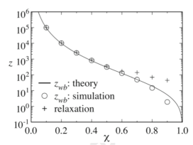
Figure 3: Comparison of the predicted time of the first wave breaking Eq.(6) (solid line), with the result of dynamics simulations (circles). Time is measured in units of $\kappa^{-1/2}$. A very good agreement between the theory and the simulations extends all the way to $\chi=0.8$. Crosses show the relaxation time — when emittance saturates. Note that up to $\chi=0.6$ the wave breaking time and the relaxation times are almost identical, see the discussion in the text.

To summarize, we have investigated the dynamics of space-charge dominated beams davidson01 with inhomogeneous density profiles. Using Lagrangian coordinates, we were able to derive a very accurate analytical expression Eq. (3) which describes very well the dynamics of beam particles, up to the wave breaking time. The fluid picture loses its validity when the propagating wave fronts result in a singular build up of density. At this point the crest of the propagating wave will break off producing an azimuthally symmetric jet of particles accelerated by the wave front. This process will repeat itself many times leading to a final stationary state in which the beam separates into a cold core surrounded by a halo of highly energetic particles. The theory presented in this paper allows to calculate precisely the time at which the wave breaking will take place. It also gives a very good estimate for the time of relaxation to the final stationary state. Unlike other systems in which the wave breaking occurs only when thresholds on driving fields are exceeded rosen02 , inhomogeneous beams are found to be always unstable hof83 and the wave breaking is unavoidable.

Wave breaking is not the only mechanism which leads to the relaxation of initially non-stationary intense particle beams. It is well known that oscillations of mismatched envelopes can be damped by the Gluckstern resonances. However, in practice, inhomogeneities are much harder to suppress than the envelope mismatches lund05 . In these cases the wave breaking described in the present letter will be the dominant mechanism by which a system reaches its final stationary state.

The theory presented here describes beams with vanishing initial emittances. One example of this are the crystalline beams for which the initial emittance is suppressed by a series of dissipative cooling procedures oka02 . We expect, however, that the theory will remain valid also for beams of initial finite emittances as long as the thermal length is small, $v_{th}z_{wb}=\varepsilon_{th}z_{wb}/2r_{b}<A\sim\chi r_{b}$, where $v_{th}=\sqrt{<v^{2}>}$ is the characteristic thermal velocity, $A$ is the characteristic amplitude of particle oscillations, and the value of the wave breaking time is given in Fig. (3). Since in general $z_{wb}\gg 1/\omega_{0}$ and $\chi<1$, the condition requires that the thermal velocity be smaller than the macroscopic velocity $\omega_{0}A$ mori88 and that the beam be space charge dominated $\varepsilon\ll K/\sqrt{\kappa}$.

This work is supported by CNPq and FAPERGS, Brazil, and by the Air Force Office of Scientific Research (AFOSR), USA, under the grant FA9550-06-1-0345.

References

- (1) A. Cuchetti, M. Reiser, and T. Wangler, in Proceedings of the Invited Papers, Particle Accelerator Conference, San Francisco, USA, 1991, edited by L. Lizama and J. Chew (IEEE, New York, 1991), Vol. 1, p. 251.
- (2) R.L. Gluckstern, Phys. Rev. Lett. 73, 1247 (1994).
- (3) R. Pakter, G. Corso, T.S. Caetano, D. Dillenburg, and F.B. Rizzato, Phys. Plasmas, 12, 4099 (1994).
- (4) R. Pakter, S.R. Lopes, and R.L. Viana, Physica D 110, 277 (1997).
- (5) R. L. Gluckstern, Proc. National Accelerator Lab. Linear Accelerator Conf., Batavia, IL, Sep. 1970, p. 811.
- (6) S. M. Lund and R. C. Davidson, Phys. Plasmas, 5, 3028 (1998).
- (7) S. Bernal, R.A. Kishek, M. Reiser, and I. Haber, Phys. Rev. Lett. 82, 4002 (1999).
- (8) S.M. Lund, D.P. Grote, and R.C. Davidson, Nuc. Instr. and Meth. A 544, 472 (2005); Y. Fink, C. Chen and W.P. Marable, Phys. Rev. E 55, 7557 (1997).
- (9) H. Okamoto and M. Ikegami, Phys. Rev. E 55, 4694 (1997).
- (10) M. Reiser, Theory and Design of Charged Particle Beams, (Wiley-Interscience, 1994); R.C. Davidson and H. Qin, Physics of Intense Charged Particle Beams in High Energy Accelerators (World Scientific, Singapore, 2001).
- (11) R. Pakter and F.B. Rizzato, Phys. Rev. Lett. 87, (2001).
- (12) D. Bruhwiler and Y.K. Batygin, in Proceedings of the PAC 1995, Dallas, TX (IEEE, Piscataway, NJ, 1995), p. 3254.
- (13) P.J. Morrison, Rev. Mod. Phys. 70, 467 (1998).
- (14) W. Braun and K. Hepp, Comm. Math. Phys. 56, 101 (1977).
- (15) Y. Levin, Rep. Prog. Phys. 65, 1577 (2002).
- (16) R.J. England, J.B. Rosenzweig, and N. Barov, Phys. Rev. E 66, 016501 (2002); T. Ohkubo, S.V. Bulanov, A.G. Zhidkov, T. Esirkepov, J. Koga, M. Uesaka, and T. Tajima, Phys. Plasmas 13, 103101 (2006).
- (17) I. Hofmann, L.J. Laslett, L. Smith, and I. Haber, Part. Accel., 13, 145 (1983).
- (18) H. Okamoto, Phys. Plasmas 9, 322 (2002).
- (19) T. Katsouleas and W.B. Mori, Phys. Rev. Lett. 61, 90 (1988).