Additional Gradings in Khovanov homology

Abstract

The main goal of the present paper is to construct new invariants of knots with additional structure by adding new gradings to the Khovanov complex. The ideas given below work in the case of virtual knots, closed braids and some other cases of knots with additional structure. The source of our additional grading may be topological or combinatorial; it is axiomatised for many partial cases. As a byproduct, this leads to a complex which in some cases coincides (up to grading renormalisation) with the usual Khovanov complex and in some other cases with the Lee-Rasmussen complex.

The grading we are going to construct behaves well with respect to some generalisations of the Khovanov homology, e.g., Frobenius extensions. These new homology theories give sharper estimates for some knot characteristics, such as minimal crossing number, atom genus, slice genus, etc.

Our gradings generate a natural filtration on the usual Khovanov complex. There exists a spectral sequence starting with our homology and converging to the usual Khovanov homology.

1 Introduction

In the last few years, the invention of link homology (Khovanov homology, Ozsváth-Szabó invariants, and also papers by Rasmussen, Khovanov-Rozansky, Manolescu-Ozsváth-Sarkar-Thurston and others) brought many constructions from algebraic topology to knot theory and low-dimensional topology.

Such theories take a representative of a low-dimensional diagram (say, knot diagram or Heegaard diagram of a 3-manifold) and associate a certain complex with this. The homology of this complex is independent of the choice of representative, thus the homology defines an invariant of knot (resp., 3-manifold, knot in a manifold). Such algebraic complexes have different gradings, and this allows one to construct filtrations and spectral sequences. The behaviour of such spectral sequences is often closely connected to some topological property of knots/3-manifolds. A nice example is the work of Rasmussen [Ras] estimating the Seifert genus from Khovanov homology and giving a simple proof of Milnor’s conjecture. Another example is the work by K.Kawamura [Kaw], who sharpened the Morton-Franks-Williams estimate for the braiding index.

There is also an approach to estimate the minimal crossing number, see [Ma8].

We shall mainly concentrate on Khovanov homology. In a sequence of recent papers, the author generalized Khovanov’s theory from knots in ${\bf R}^{3}$ to knots in arbitrary thickened $2$-surfaces (up to stabilisation, giving virtual knots (by Kauffman, [KaV]) or twisted knots (by Bourgoin,[Bou])).

Virtual knots, besides their “knottedness” also carry some information about the topology of the underlying surface.

Thus, it would be quite natural to take into account some topological data to introduce into Khovanov homology to make the latter stronger. This idea was also used in the paper by Asaeda, Przytycki, Sikora [APS]. We shall discuss the interaction between the present work and the work [APS] later.

The main idea goes as follows: Assume we have a well-defined complex made out of some knot diagram. Consider the chain spaces ${\cal C}(K)$ and the differential $\partial$. It turns out that in some cases it is possible to introduce a new grading $gr$ that splits the differential $\partial$ into two parts $\partial=\partial^{\prime}+\partial^{\prime\prime}$ in such a way that:

1. $\partial^{\prime}$ preserves the new grading, whence $\partial^{\prime\prime}$ increases the new grading;

2. $(C,\partial^{\prime})$ is a well-defined complex;

3. the homology of $(C,\partial^{\prime})$ is invariant (under Reidemeister moves);

4. there is a spectral sequence with $E^{1}=H(C,\partial)$ converging to the usual Khovanov homology (the latter differential is taken with respect to $\partial$).

The new gradings have a topological nature: they correspond to cohomology classes.

This will guarantee that the complex is well defined. However, the gradings may be of any other (say, combinatorial) nature; the only thing we need is that for the Kauffman bracket states, there are two sorts of circles which behave nicely with respect to the Reidemeister moves.

The latter condition guarantees not only that the complex is well defined (that is, $\partial^{\prime}$ is indeed a differential) but also the invariance under Reidemeister moves.

Varying this construction, one can construct further complexes with differentials of type $\partial^{\prime}+\lambda\partial^{\prime\prime}$, where $\lambda$ can be a coefficient or some operator.

The outline of the present paper is the following. In the next section, we define the Kauffman bracket, virtual knots, and Khovanov homology (with arbitrary coefficients) for virtual links and classical links (which actually constitute a proper part of virtual links).

Section 3 will be devoted to our main example: categorifying the Bourgoin invariant with the only one new grading corresponding to the first Stiefel-Whitney class for oriented thickenings of non-orientable surfaces.

The proof of the invariance theorem is given in section 4; it indeed contains all ingredients for the proof of the main theorem to follow in section 5, where we have multiple gradings of various types and present more examples.

Section 5 also contains the axiomatics for these new gradings and examples what they can be applied to: braids, cables, tangles, long knots etc.

Section 6 devoted is to a generalisation of Khovanov’s Frobenius structure. From this point of view, one can think of Lee’s homology as a partial case of Khovanov’s Frobenius theory as well as our new theory. As a byproduct, we present yet another definition of the Khovanov theory where the usual gradings are treated from our “dotted grading viewpoint”.

In section 7, we focus on gradings and filtrations. We discuss the Frobenius construction due to Khovanov, which is then followed by spectral sequences, and Lee-Rasmussen invariants.

Section 8 is devoted to applications of the theory constructed and generalisations of some classical constructions in this context

Section 9 is devoted to the discussion and open questions.

1.1 Acknowledgments

I am very grateful to O.Ya.Viro for various stimulating discussions. During the writing process of that paper, I also had very useful discussions with L.H.Kauffman, V.A.Vassiliev, M.Khovanov, J.H.Przytycki, V.G.Turaev.

2 Preliminaries: Virtual knots, Kauffman bracket, atoms, and Khovanov homology

We think of knot diagrams as a collection of (classical) crossings on the plane somehow connected by arcs, see Fig. 1.

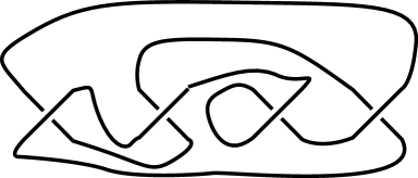
Figure 1: A knot diagram

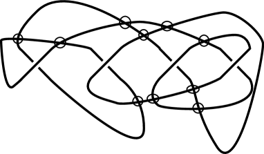
Figure 4: A virtual diagram

Knots are such diagrams modulo Reidemeister moves, but sometimes it happens that for a given setup of crossings we are unable to connect them by arcs in an appropriate way; this will lead to a diagram called virtual with artefacts of the projection encircled, see Fig. 4.

2.1 Atoms and Knots

A four-valent planar graph $\Gamma$ generates a natural checkerboard colouring of the plane by two colours (adjacent components of the complement ${\bf R}^{2}\backslash\Gamma$ have different colours).

This construction perfectly describes the role played by alternating diagrams of classical knots. Recall that a link diagram is alternating if while walking along any component we alternate over= and underpasses. Another definition of an alternating link diagram sounds as follows: fix a checkerboard colouring of the plane (one of the two possible colourings). Then, for every vertex the colour of the region corresponding to the angle swept by going from the overpass to the underpass in the counterclockwise direction is the same.

Thus, planar graphs with natural colourings somehow correspond to alternating diagrams of knots and links on the plane: starting with a graph and a colouring, we may fix the rule for making crossings: if two edges share a black angle, then the we decree the left one (with respect to the clockwise direction) to form an overcrossing, and the right one to be an undercrossing, see Fig. 2. Thus, colouring a couple of two opposite angles corresponds to a choice of a pair of opposite edges to form an overcrossing and vice versa.

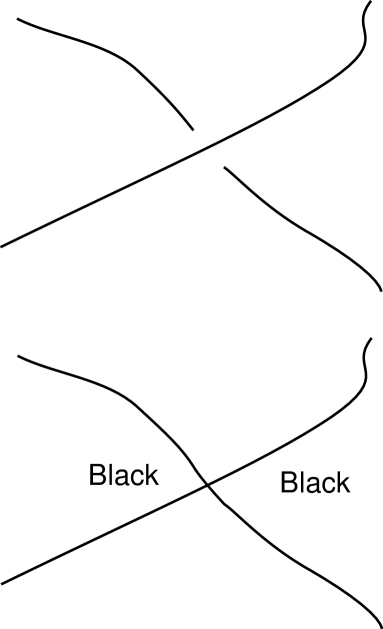
Figure 2: A crossing corresponding to a vertex of an atom

Now, if we take an arbitrary link diagram and try to establish the colouring of angles according to the rule described above, we see that generally it is impossible unless the initial diagram is alternating: we can just get a region on the plane where colourings at two adjacent angles disagree. So, alternating diagrams perfectly match colourings of the $2$-sphere (think of $S^{2}$ as a one-point compactification of ${\bf R}^{2}$). For an arbitrary link, we may try to take colours and attach cells to them in a way that the colours would agree, namely, the circuits for attaching two-cells are chosen to be those rotating circuits, where we always turn inside the angle of one colour.

This leads to the notion of atom. An atom is a pair $(M,\Gamma)$ of a $2$-manifold $M$ and a graph $\Gamma$ embedded $M$ together with a colouring of $M\backslash\Gamma$ in a checkerboard manner. Here $\Gamma$ is called the frame of the atom, whence by genus (resp., Euler characteristic) of the atom we mean that of the surface $M$.

Note that the atom genus is also called the Turaev genus, [TuraevGenus].

Certainly, such a colouring exists if and only if $\Gamma$ represents the trivial ${\bf Z}_{2}$ homology class in $M$.

Thus, gluing cells to some turning circuits on the diagram, we get an atom, where the shadow of the knot plays the role of the frame. Note that the structure of opposite half-edges on the plane coincides with that on the surface of the atom.

Now, we see that atoms on the sphere are precisely those corresponding to alternating link diagrams, whence non-alternating link diagrams lead to atoms on surfaces of a higher genus.

In some sense, the genus of the atom is a measure of how far a link diagram is from an alternating one, which leads to generalisations of the celebrated Kauffman-Murasugi theorem, see [MyBook] and to some estimates concerning the Khovanov homology [Ma8].

Having an atom, we may try to embed its frame in ${\bf R}^{2}$ in such a way that the structure of opposite half-edges at vertices is preserved. Then we can take the “black angle” structure of the atom to restore the crossings on the plane.

In [AtomsAndKnots] it is proved that the link isotopy type does not depend on the particular choice of embedding of the frame into ${\bf R}^{2}$ with the structure of opposite edges preserved. The reason is that such embeddings are quite rigid.

The atoms whose frame is embeddable in the plane with opposite half-edge structure preserved are called height or vertical.

However, not all atoms can be obtained from some classical knots. Some abstract atoms may be quite complicated for its frame to be embeddable into ${\bf R}^{2}$ with the opposite half-edges structure preserved. However, if it is impossible to immerse a graph in ${\bf R}^{2}$, we may embed it by marking artifacts of the embedding (we assume the embedding to be generic) by small circles.

A virtual diagram is a four-valent graph on the plane with two types of crossings: classical or (for which we mark which pair of opposite edges form an overpass) and virtual (which are just marked by a circled crossing).

A virtual link is an equivalence class of virtual diagrams modulo generalised Reidemeister moves. The later consist of usual Reidemeister moves and the detour move. The detour move removes an arc virtually connecting some points $A$ and $B$ (that is, having no classical crossings inside) restores another connection between $A$ and $B$ with several virtual intersections and self-intersections, see Fig. 3.

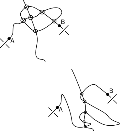
Figure 3: The detour move

This move just means that it is inessential to indicate which curves connect classical crossings, it is important only to know how these crossings are paired.

Considering these diagrams modulo usual Reidemeister moves and the detour moves (see ahead), we get what are called virtual knots. The detour move is the move removing an arc (possibly, with self-intersections) containing only virtual crossing, and adding another arc connecting the same points elsewhere.

Virtual knots, being defined diagrammatically, have a topological interpretation. They correspond to knots in thickened surfaces $S_{g}\times I$ with fixed $I$-bundle structure (later we will also talk about oriented thickenings of non-orientable surfaces) up to stabilisations/destabilisations. Projecting $S_{g}$ to ${\bf R}^{2}$ (with the condition, however, that all neighbourhoods of crossings are projected with respect to the orientation, we get from a generic diagram on $S_{g}$ a diagram on ${\bf R}^{2}$: besides the usual crossings arising naturally as projections of classical crossings, we get virtual crossings, which arise as artefacts of the projection: two strands lie in different places on $S_{g}$ but they intersect on the plane because they are forced to do so.

Having a (virtual) knot diagram, we can smooth all classical crossings of it in the following two ways: $A:\mbox{\raisebox{-0.25pt}{\includegraphics[width=14.22636pt]{skcrossr.eps}}}\to\mbox{\raisebox{-0.25pt}{\includegraphics[width=14.22636pt]{skcrh.eps}}}$ and $B:\mbox{\raisebox{-0.25pt}{\includegraphics[width=14.22636pt]{skcrossr.eps}}}\to\mbox{\raisebox{-0.25pt}{\includegraphics[width=14.22636pt]{skcrv.eps}}}$.

Thus, for a diagram $L$ with $n$ classical crossings we have $2^{n}$ states. Every state is a way of smoothing all (classical) crossings. Enumerate all classical crossings by $1,\dots,n$. Then the states can be regarded as vertices of the discrete cube $\{0,1\}^{n}$, where $0$ and $1$ correspond to the $A$-smoothing and the $B$-smoothing, respectively. In each state we have a collection of circles representing an unlink. We call this cube the state cube of the diagram $L$.

Then any for any state $s$ we have its height $\beta(s)$ being the number of crossings resolved positively, $\alpha(s)=n-\beta(s)$ being the number of crossings resolved negatively, and the number $\gamma$ of closed circles.

Then the Kauffman bracket is defined as

$$\sum_{s}a^{\alpha(s)-\beta(s)}(-a^{2}-a^{-2})^{\gamma(s)-1}$$ (1)

This bracket is invariant under all Reidemeister moves except for the first one.

The normalisation $X(K)=(-a)^{-3w(K)}\langle K\rangle$, where $w$ is the writhe number, leads to the definition of the Jones polynomial.

The Kauffman bracket satisfies the usual relation

$$\langle\raisebox{-0.25pt}{\includegraphics[width=14.22636pt]{skcrossr.eps}}\rangle=a\langle\raisebox{-0.25pt}{\includegraphics[width=14.22636pt]{skcrv.eps}}\rangle+a^{-1}\langle\raisebox{-0.25pt}{\includegraphics[width=14.22636pt]{skcrv.eps}}\rangle$$ (2)

After a little variable change and renormalisation, the Kauffman bracket can be rewritten in the following form:

$$\langle\raisebox{-0.25pt}{\includegraphics[width=14.22636pt]{skcrossr.eps}}\rangle=\langle\raisebox{-0.25pt}{\includegraphics[width=14.22636pt]{skcrv.eps}}\rangle-q\langle\raisebox{-0.25pt}{\includegraphics[width=14.22636pt]{skcrv.eps}}\rangle$$ (3)

Here we consider bigraded complexes ${\cal C}^{ij}$ with height (homological grading) $i$ and quantum grading $j$; the differential preserves the quantum grading and increases the height by $1$. The height and grading shift operations are defined as $({\cal C}[k]\{l\})^{ij}={\cal C}[i-k]\{j-l\}$.

This form is used as the starting point for the Khovanov homology. Namely, we regard the factors $(q+q^{-1})$ as graded dimensions of the module $V=\{1,X\},\mbox{deg}\;1=1,\mbox{deg}\;X=-1$ over some ring $R$, and the height $\beta(s)$ plays the role of homological dimension. Then, if we define the chain space $[[K]]_{k}$ of homological dimension $k$ to be the direct sum over all vertices of $\beta=k$ of $V^{\gamma(s)}\{k\}$ (here $\{\cdot\}$ is the quantum grading shift), then the alternating sum of graded dimensions of $[[K]]_{k}$, is precisely equal to the (modified) Kauffman bracket.

Thus, if we define a differential on $[[K]]$ preserving the grading and increasing the homological dimension by $1$, the Euler characteristic of that space would be precisely the Kauffman bracket.

Remark 1.

Later on, we shall not care about the normalisation of the complexes by degree and height shifts to make their homology invariant under the Reidemeister moves. It is done exactly as in [Kh].

We have defined the state cube consisting of circles and carrying no information how these circles interact. Turning to Khovanov homology, we shall deal with the same cube remembering the information about the circle bifurcation. Later on, we refer to it as a bifurcation cube.

The chain spaces of the complex are well defined. However, the problem of finding a differential $\partial$ in the general case of virtual knots, is not very easy. To define the differential, we have to pay attention to different isomorphism classes of the chain space identified by using some local bases.

The differential acts on the chain space as follows: it takes a chain corresponding to a certain vertex of the bifurcation cube to some chains corresponding to all adjacent vertices with greater homological degree. That is, the differential is a sum of partial differentials, each partial differential acts along an edge of the cube. Every partial differential corresponds to some direction and is associated with some classical crossing of the diagram.

With each circle, we associate the tensor power of the space $V$ of graded dimension $q+q^{-1}$, however, with no prefixed basis. With a collection of circles, we shall associate the exterior power of this space, as follows. With each state $s$ of height $b$, we associate a basis consisting of $2^{\gamma(s)}$ chains. Now, we order the circles in the state $s$ arbitrarily, fix an arbitrary orientation on them and associate with each such circle either $1$ or $X$. With any such choice, consisting of a state, an ordering of oriented circles and a set of elements $1$ and $X$, we associate a chain of the complex. We can also associate elements $\pm 1$ or $\pm X$ with any circle, which also defines a chain of our complex; this chain differs from the corresponding chain with $1$ and $X$ by a corresponding sign. Furthermore, we identify the chains according to the following rule: the orientation change for one circle leads to a sign change of a chain if this circle is marked by $\pm X$ and does not change sign if the circle is marked by $\pm 1$; the permutation of circles multiplies the chain by the sign of corresponding permutation. This would correspond to taking exterior product of vector spaces (graded modules) instead of their symmetric product.

Then for a state with $l$ circles, we get a vector space (module) of dimension $2^{l}$. All these chains have homological dimension $b$. We set the grading of these chains equals $b$ plus the number of circles marked by $1$ minus the number of circles marked by $X$.

Let us now define the partial differentials of our complex. First, we think of each classical crossing so that its edges are oriented upwards, as in Fig. 5, upper right picture.

Choose a certain state of a virtual link diagram $L\subset{\cal M}$. Choose a classical crossing $U$ of $L$. We say that in a state $s$ a state circle $\gamma$ is incident to a classical crossing $X$ if at least one of the two local parts of smoothed crossing $X$ belongs to $\gamma$. Consider all circles $\gamma$ incident to $U$. Fix some orientation of these circles according to the orientation of the edge emanating in the upward-right direction and opposite to the orientation of the edge coming from the bottom left, see Fig. 5. Such an orientation is well defined except for the case when one edge corresponding to a vertex of the cube, takes one circle to one circle. In such situation, we shall not define the local basis $\{1,X\}$; we set the partial differential corresponding to the edge, to be zero.

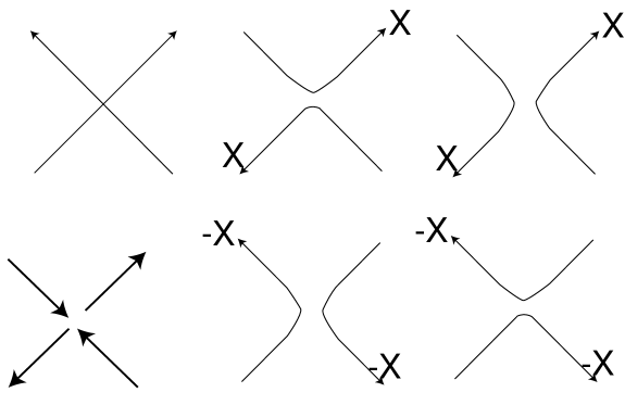
Figure 5: Setting the local basis for a crossing

In the other situations, the edge of the cube corresponding to the partial differential either increases or decreases the number of circles. This means that at the corresponding crossing the local bifurcation either takes two circles into one or takes one circle into two. If we deal with two circles incident to a crossing from opposite signs, we order them in such a way that the upper (resp., left) one is the first one; the lower (resp., right) one is the second; here the notions “left, right, upper, lower” are chosen according to the rule for identifying the crossing neighbourhood with Fig. 5. Furthermore, for defining the partial differentials of types $m$ and $\Delta$ (which correspond to decreasing/increasing the number of circles by one) we assume that the circles we deal with are in the very initial poisitions in our ordered tensor product; this can always be achieved by a preliminary permutation, which, possibly leads to a sign change. Now, let us define the partial differential locally according to the prescribed choice of generators at crossings and the prescribed ordering.

Now, we describe the partial differentials $\partial^{\prime}$ from [Ma6] without new gradings. If we set $\Delta(1)=1_{1}\wedge X_{2}+X_{1}\wedge 1_{2};\Delta(X)=X_{1}\wedge X_{2}$ $m(1_{1}\wedge 1_{2})=1;m(X_{1}\wedge 1_{2})=m(1_{1}\wedge X_{2})=X;m(X_{1}\wedge X_{2})=0$, define the partial differential $\partial^{\prime}$ according to the rule $\partial^{\prime}(\alpha\wedge\beta)=m(\alpha)\wedge\beta$ (in the case we deal with a $2\to 1$-buifurcation, where $\alpha$ denotes the first two circles $\alpha$) or $\partial^{\prime}(\alpha\wedge\beta)=\Delta(\alpha)\wedge\beta$ (when one circle marked by $\alpha$ bifurcates to two ones); here by $\beta$ we mean an ordered set of oriented circles, not incident to the given crossings; the marks on these circles $\pm 1$ and $\pm X$ are given.

Theorem 1.

[Ma6] $[[K]]$ is a well-defined complex with respect to $\partial$; after a small grading shift and a height shift, the homology is invariant under generalised Reidemeister moves.

Later, when we have new gradings, the differential will be defined just by projecting this differential to the grading-preserving subspace, namely, $\tilde{\partial}^{\prime}\alpha=\mbox{pr}_{\mbox{deg}=\mbox{deg}\alpha}\partial^{\prime}\alpha$, where $\mbox{pr}_{\mbox{deg}=\mbox{deg}\alpha}$ is the projection to the subspace having all additional gradings the same as $\alpha$. After all, we shall define $\partial$ as the sum of partial differentials $\tilde{\partial}^{\prime}$. We will get a set of graded groups $Kh^{\prime}_{H}$ with differential $\partial$. This differential increases the height (homological grading), preserves the grading, and does not change the additional gradings.

Remark 2.

The homology theory described above is initially constructed out of planar diagrams; thus, it represents a homology theory for links in thickened surfaces modulo stabilisation; that is, this homology theory “does not feel” removable handles. However, when we impose new gradings, we will have to fix the thickened surface, since we will deal with its homology groups. The new complex to be constructed for such thickened surfaces, frankly speaking, would not be a virtual link invariant. It would rather be an obstruction for links in thickened surfaces to decrease the underlying genus of the corresponding surface.

2.2 Usual Khovanov homology

For the case of classical knot theory (and also some parts of virtual knot theory) the above setup is actually not needed for constructing Khovanov homology. One can get the chain spaces generated by tensor powers of $V$ with appropriate grading and degree shifts, with no care about signs as it was done in the original Khovanov paper [Kh]. Namely, one takes just the symmetric tensor power $V^{\otimes k}$ for a vertex of a cube with $k$ circles in the corresponding state. One also need not care about signs: the type-$X$ generators are chosen once forever. Then it allows to construct partial differentials just by using some concrete formulae for $\Delta$ and $\mu$. The main difficulty we had to overcome was the case of $1\to 1$-type partial differentials. If no such $1\to 1$-bifurcations occur then the original construction works straightforwardly. Namely, after splicing some minus signs, these formulae lead to a well defined complex whose homology is the usual Khovanov homology.

The main goal of the present paper would be to find such additional gradings.

3 Bourgoin’s twisted knots.
Additional gradings

Assume for some category (knots, virtual knots, braids, tangles) we have a well-defined Kauffman bracket. That is, we have a set of (classical) crossings, which can be smoothed so that the formula (3) can be applied.

Consider the following generalisation of virtual knots (proposed by Mario Bourgoin, see [Bou]).

We consider knots in oriented thickenings of $2$-surfaces, the latter not necessarily orientable. Namely, we take a $2$-surface $M$ and fix the $I$-bundle ${\cal M}$ over $M$ which is oriented as a total fibration space, and keep both the orientation and the $I$-bundle structure fixed.

We consider knots and links in such surfaces up to stabilisation/destabilisation and refer to them as twisted links. Virtual links constitute a proper part of twisted links [Bou].

Note that this theory encloses as a partial case the theory of knots in ${\bf R}P^{3}$, since ${\bf R}P^{3}\backslash\{*\}$ is nothing but the oriented thickening of ${\bf R}P^{2}$.

Any link in ${\cal M}$ has a projection to the base space, the latter being a four-valent graph.

Since the surface is orientable (and even oriented), there is a canonical way for defining the $A$-smoothing and the $B$-smothing with respect to the orientation. Thus, the formula (3) gives a well-defined Kauffman bracket for such objects, which turns out to be invariant; the proof is standard, see, e.g. [Ma3].

Moreover, the approach described in the previous section gives a well-defined Khovanov homology theory. To this end, we have to establish the chain space and the differentials.

Fix a cell decomposition of $M$ with exactly one $2$-cell $C$ and choose a canonical “upward” direction for $C$. Then we can treat every crossing as a classical one, that is, identify its neighbourhood with the local picture shown in Fig. 5.

This allows to define $[[K]]$ literally as above, and we get the following

Theorem 2.

For twisted knots the complex $[[K]]$ is a well-defined complex with respect to $\partial^{\prime}$; after a small grading shift and a height shift, the homology is invariant under isotopy (the orientation of the ambient space remains fixed together with the $I$-bundle structure); the differential $\partial^{\prime}$ increases the homological grading by $1$ and preserves the quantum grading and the additional gradings.

As shown in [Ma6], the homology of this complex does not depend on the choice of $C$ and the upward orientation.

We should mention, that there have been a lot of generalisations of the Kauffman bracket, see e.g. Kauffman-Dye [DK2], Manturov [Ma9], Miyazawa [Miy].

Each of these generalisations introduces something new to the formula for the Kauffman bracket of either topological or combinatorial nature.

Bourgoin proposed the following generalization of the Kauffman bracket for such surfaces.

$$\sum_{s}a^{\alpha(s)-\beta(s)}M^{\gamma^{\prime\prime}(s)}(-a^{2}-a^{-2})^{\gamma^{\prime}(s)}$$ (4)

where $\gamma^{\prime}$ and $\gamma^{\prime\prime}$ correspond to the number of orienting/non-orienting circles in the state $s$, respectively.

The goal of the present section is to describe how to categorify this invariant and then see which further examples will fit into the construction.

In the Khovanov setup, we had $(q+q^{-1})$ instead of $(-a^{2}-a^{-2})$. What should we have instead of $M$?

What should be the vector space categorifying this variable. As can be seen from Khovanov’s algebraic reasonings, see [Kh2], the space corresponding to one circle should be two-dimensional.

To preserve the similarity with the initial picture, it is convenient to make one generator $(1)$ of this space having quantum grading $q$ and the other one (which might be $X$ or $-X$) having quantum grading to $q^{-1}$.

This is the point where new gradings come into play: with every non-orienting circle in a Kauffman state, we associate the space of graded dimension $qg^{-1}+q^{-1}g$, where $g$ corresponds to the new grading. At the uncategorified level, this just means $M=qg^{-1}+q^{-1}g$, and thus we lose no information.

At the categorified level, this means that we introduce a new grading for the spaces: for every non-orienting loop we associate a $Z$-grading equal to $1$ if this loop is marked by $X$ and $-1$ if this loop is marked by $1$. For orienting loops, we have no new gradings.

Now, let us define the new grading ($g$-grading) for the complex $[[K]]$ as the sum of all new gradings over all non-orienting circles.

Denote the obtained complex by $[[K]]_{g}$; this is actually nothing but $[[K]]$ with new grading imposed.

$\dot{1}$

Notation. Further on, we shall mark all labels belonging to non-orienting circles by a point, that is, we write $11$ and $\dot{X}$ for labels $1$ and $X$ on non-orienting circles.

Here we give an example how one smoothing with dots gets reconstructed into another smoothing; we put dots over some circles which correspond to “non-orienting” curves, see Fig. 3.

Let us look how the differentials in $[[K]]$ behave with respect to the new grading $g$. It is easy to see that

Lemma 1.

The differential $\partial$ can be uniquely represented as $\partial^{\prime}+\partial^{\prime\prime}$, where $\partial^{\prime}$ preserves the new grading, and $\partial^{\prime\prime}$ increases the new grading by $2$.

Indeed, one can check all $m$-type and $\Delta$-type differentials, and see that $11\wedge 11\to 1$, $11\wedge X\to\mbox{$\dot{X}$}$, $X\to\mbox{$\dot{X}$}\wedge\mbox{$\dot{X}$}$ are all increasing the grading by $2$, whence the differential $11\to X\wedge 11+1\wedge\mbox{$\dot{X}$}$ splits into two parts, where the first one preserves the new grading, and the second one increases that by $2$.

From Lemma 1 we get

Lemma 2.

$[[K]]_{g}$ is a well defined triply graded complex with respect to the differential $\partial^{\prime}$.

Proof.

Indeed, $({\partial^{\prime}}^{2})$ is just the projection of $\partial^{2}=0$ to the grading-preserving subspace. ∎

Luckily, it turns out that the homology of $[[K]]_{g}$ is invariant after the same grading and degree shift (for old gradings) as in the usual case of classical knots ([Kh]) or virtual knots with oriented atoms [Ma3]. We shall show this more generally in the next section.

4 Additional grading: the general case

The goal of our section is the following. Assume we have a space of knots (braids, tangles, etc.) with a well-defined Kauffman bracket and Khovanov homology. We wish to mark some circles in Kauffman’s states by dots (analogously to non-orienting cirlces in Bourgoin’s case) thus defining the new “dotted gradings”: the dotted grading for the state is defined as the number of all $\dot{X}$ minus the number of all $11$. Then we split the usual Khovanov differential $\partial$ into two parts: the one $\partial^{\prime}$ preserving the dotted grading and the one $\partial^{\prime\prime}$ changing the dotted grading.

What are the properties this dotting should satisfy if we want the grading to satisfy the following:

1. The complex $[[K]]_{g}$ is well defined;

2. Its homology (after some height and degree shift) is invariant under isotopy (combinatorial equivalence, Reidemeister moves).

The answer to the first question is easy: we just need that $\partial^{\prime\prime}$ either always increase the new grading or always decrease the new grading. Then it will guarantee $\partial^{\prime 2}=0$.

But if we want the dots on circles to behave just as in the case of Bourgoin so that the rules for multiplication and comultiplication (with respect to the new grading) are:

$$m(1\wedge 1)=1;m(1\wedge X)=X;m(X\wedge 1)=X;m(X\wedge X)=0$$

$$m(11\wedge 1)=11;m(11\wedge X)=0;m(\mbox{$\dot{X}$}\wedge 1)=\mbox{$\dot{X}$};m(\mbox{$\dot{X}$}\wedge X)=0$$

$$m(1\wedge 11)=11;m(1\wedge\mbox{$\dot{X}$})=\mbox{$\dot{X}$};m(X\wedge 11)=0;m(X\wedge\mbox{$\dot{X}$})=0$$

$$m(11\wedge 11)=0;m(11\wedge\mbox{$\dot{X}$})=X;m(\mbox{$\dot{X}$}\wedge 11)=X;m(\mbox{$\dot{X}$}\wedge\mbox{$\dot{X}$})=0$$

and

$$\Delta(1)=1\wedge X+X\wedge 1$$

or

$$\Delta(1)=11\wedge\mbox{$\dot{X}$}+dX\wedge 1$$

(depending on whether the output circles are dotted)

$$\Delta(X)=X\wedge X$$

or (when both output circles are dotted)

$$\Delta(X)=0.$$

$$\Delta(11)=11\wedge X$$

or

$$\Delta(11)=\mbox{$\dot{X}$}\wedge 11$$

(depending on which of the two output circles is dotted)

$$\Delta(\mbox{$\dot{X}$})=X\wedge\mbox{$\dot{X}$}$$

or

$$\Delta(X)=\mbox{$\dot{X}$}\wedge X$$

(depending on which of the two output circles is dotted).

The operators $m$ and $\Delta$ above are just as before (in the categorification of Bourgoin’s invariant), however, with the reasons for putting dots completely forgotten.

Nevertheless, to have precisely this dotting, we need that the dotting of circles is additive modulo ${\bf Z}_{2}$, that is, if we have a $2\to 1$ bifurcation, then the number of dots for the two circles is congruent modulo $2$ to the number of dots for the one circle (analogously for $1\to 2$-bifurcations). We also require that this dotting is preserved under $1\to 1$-bifurcations, that is, if a surgery transforms one circle to one circle then this circle should necessarily be unorienting both before and after the surgery.

The conditions above is enough for the complex $[[K]]_{g}$ to be well defined.

Now, in order to have the invariance under the Reidemeister moves, we have to restore the proof picture of Khovanov (or of [Ma6]).

The invariance under the first Reidemeister move is based on the following two which should held when adding a small curl:

1. the mapping $\Delta$ is injective

2. the mapping $m$ is surjective.

In fact, the last two conditions hold when the small circle is not dotted.

Indeed, consider the complex

$$[[\raisebox{-0.25pt}{\includegraphics[width=14.22636pt]{skkinkr.eps}}]]=\left([[\raisebox{-0.25pt}{\includegraphics[width=14.22636pt]{skroh.eps}}]]\stackrel{{\scriptstyle m}}{{\to}}[[\raisebox{-0.25pt}{\includegraphics[width=14.22636pt]{skrov.eps}}]]\{1\}\right).$$ (5)

The usual argument goes as follows: the complex in the right hand side contains a $\Delta$-type partial differential, which is injective. Thus, the complex $[\raisebox{-0.25pt}{\includegraphics[width=14.22636pt]{skrov.eps}}]]$ is killed, and what remains from $[\raisebox{-0.25pt}{\includegraphics[width=14.22636pt]{skroh.eps}}]]$ is precisely (after a suitable normalisation) the homology of $[[\raisebox{-0.25pt}{\includegraphics[width=14.22636pt]{skkinkl.eps}}]]$.

But $\Delta$ is injective because for any $l\in{1,X}$ we have $\Delta(l)=l\wedge X+\langle somemess\rangle$, where the second term $X$ in $l\wedge X$ corresponds to the small circle.

But in our situation with dotted circles, this happens only if the small circle is not dotted. But if the small circle is dotted, it would lead, say, to $\Delta:X\to 0$, because $\mbox{$\dot{X}$}\wedge\mbox{$\dot{X}$}$ has another dotted grading (greater by $2$ than the grading of $X$). But when the small circle is dotted, the proof is the same.

An analogous situation happens with

$$[[\raisebox{-0.25pt}{\includegraphics[width=14.22636pt]{skkinkl.eps}}]]=\left([[\raisebox{-0.25pt}{\includegraphics[width=14.22636pt]{skrov.eps}}]]\stackrel{{\scriptstyle m}}{{\to}}[[\raisebox{-0.25pt}{\includegraphics[width=14.22636pt]{skroh.eps}}]]\{1\}\right).$$ (6)

Here we need that the mapping $m$ be surjective; actually, it would suffice that the multiplication by $1$ on the small circle is the identity. But this happens if and only if the small circle is not dotted, that is, we have $1$, not $11$.

Quite similar things happen for the second and for the third Reidemeister moves. The necessary conditions can be summarised as follows:

The small circles which appear for the second and the third Reidemeister move should not be dotted.

The explanation comes a bit later. Now, we see that this condition is obviously satisfied when the dotting comes from a cohomology class, and not necessarily the Stiefel-Whitney cohomology class for non-orientable surface. Any homology class should do.

Thus (modulo some explanations given below) we have proved the following

Theorem 3.

Let ${\cal M}\to M$ be a fibration with $I$-fibre so that ${\cal M}$ is orientable and $M$ is a $2$-surface. Let $h$ be a $Z_{2}$-cohomology class and let $g$ be the corresponding dotting. Consider the corresponding grading on $[[K]]$. Then for a link $K\subset{\cal M}$ the homology of $[[K]]_{g}$ is invariant under isotopy of $K$ in $M$ (with both the orientation of $M$ and the $I$-bundle structure fixed) up to some shifts of the usual (quantum) grading and height (homological grading).

4.1 Explanation for the second and the third moves

We have the following picture for the Reidemeister move for $[[\raisebox{-0.25pt}{\includegraphics[width=14.22636pt]{skrtwhh.eps}}]]$:

$$\begin{array}[]{ccc}\mbox{[[}\raisebox{-0.25pt}{\includegraphics[width=14.22636pt]{skrtwhh.eps}}\mbox{]]}\{1\}&\stackrel{{\scriptstyle m}}{{\longrightarrow}}&\mbox{[[}\raisebox{-0.25pt}{\includegraphics[width=14.22636pt]{skrtwvh.eps}}\mbox{]]}\{2\}\\ \Delta\uparrow&&\uparrow\\ \mbox{[[}\raisebox{-0.25pt}{\includegraphics[width=14.22636pt]{skrtwhv.eps}}\mbox{]]}&\longrightarrow&\mbox{[[}\raisebox{-0.25pt}{\includegraphics[width=14.22636pt]{skrtwvv.eps}}\mbox{]]}\{1\}\end{array}.$$ (7)

Here we use the notation ${\{\cdot\}}$ for the degree shifts, see page 4.

$$\begin{array}[]{ccc}\mbox{[[}\raisebox{-0.25pt}{\includegraphics[width=14.22636pt]{skrtwhh.eps}}\mbox{]]}\{1\}&\stackrel{{\scriptstyle m}}{{\longrightarrow}}&\mbox{[[}\raisebox{-0.25pt}{\includegraphics[width=14.22636pt]{skrtwvh.eps}}\mbox{]]}\{2\}\\ \Delta\uparrow&&\uparrow\\ \mbox{[[}\raisebox{-0.25pt}{\includegraphics[width=14.22636pt]{skrtwhv.eps}}\mbox{]]}&\longrightarrow&\mbox{[[}\raisebox{-0.25pt}{\includegraphics[width=14.22636pt]{skrtwvv.eps}}\mbox{]]}\{1\}\end{array}.$$ (8)

This complex contains the subcomlex ${\cal C}^{\prime}$:

$${\large{\cal C}^{\prime}}=\begin{array}[]{ccc}\mbox{[[}\raisebox{-0.25pt}{\includegraphics[width=14.22636pt]{skrtwhh.eps}}\mbox{]]}_{1}\{1\}&\stackrel{{\scriptstyle m}}{{\longrightarrow}}&\mbox{[[}\raisebox{-0.25pt}{\includegraphics[width=14.22636pt]{skrtwvh.eps}}\mbox{]]}\{2\}\\ \uparrow&&\uparrow\\ 0&\longrightarrow&0\end{array}$$ (9)

if the small circle is not dotted.

Here and further $1$ denotes the mark on the small circle.

Then the acyclicity of ${\cal C}^{\prime}$ is evident.

Factoring ${\cal C}$ by ${\cal C^{\prime}}$, we get:

$$\begin{array}[]{ccc}\mbox{[[}\raisebox{-0.25pt}{\includegraphics[width=14.22636pt]{skrtwhh.eps}}\mbox{]]}\{1\}/_{1=0}&\longrightarrow&0\\ \Delta\uparrow&&\uparrow\\ \mbox{[[}\raisebox{-0.25pt}{\includegraphics[width=14.22636pt]{skrtwhv.eps}}\mbox{]]}&\longrightarrow&\mbox{[[}\raisebox{-0.25pt}{\includegraphics[width=14.22636pt]{skrtwvv.eps}}\mbox{]]}\{1\}\end{array}.$$ (10)

In the last complex, the mapping $\Delta$ directed upwards, is an isomorphism (when our small circle is not dotted). Thus the initial complex has the same homology group as $[[\raisebox{-0.25pt}{\includegraphics[width=14.22636pt]{skrtwvv.eps}}]]$. This proves the invariance under $\Omega_{2}$.

The argument for $\Omega_{3}$ is standard as well; it relies on the invariance under $\Omega_{2}$ and thus we should also require that the small circle is not dotted.

5 More gradings; more examples

We have listed the necessary conditions for the dotting to give such a grading that $[[K]]_{g}$ is invariant (up to some shifts); the conditions are quite natural: additivity of dots modulo ${\bf Z}_{2}$ and triviality of small circles for all types of Reidemeister moves. We have actually missed one condition we assumed without saying. Namely, in the pictures corresponding to the Reidemeister moves, the similar arcs are dotted similarly.

This means, for example, that for the second Reidemeister move the smoothing gives two branches which should have the same dotting as the two branches of . The same follows for all the three moves.

Thus, we introduce the dotting axiomatics. Namely, assume we have some class of objects with Reidemeister moves, Kauffman bracket and the Khovanov homology (in the usual setup or in the setup of [Ma6]). Assume its circles can be dotted in such a way that the following conditions hold:

1. The dotting of circles is additive with respect to $2\to 1$-bifurcations, and it is preserved under $1\to 1$-bifurcations.

2. Similar curves for similar smoothings of the RHS and the LHS of any Reidemeister move have the same dotting

   and

3. Small circles appearing for the first, the second, and the third Reidemeister moves are not dotted.

Let us call the conditions above the dotting conditions.

Theorem 4.

Assume there is a theory with Khovanov complex $([[K]],\partial)$ such that the Kauffman states can be dotted so that the dotting conditions hold. Define $[[K]]_{g}$ as before (see page 2).

1) Then the homology of $[[K]]_{g}$ is invariant (up to a degree shift and a height shift).

2) For any operator $\lambda$ on the ground ring, the complex $[[K]]_{g}$ is well defined with respect to the differential $\partial^{\prime}+\lambda\partial^{\prime\prime}$, and the corresponding homology is invariant (up to well-known shifts).

3) Moreover, if we have several dottings $g_{1},g_{2},\dots,g_{k}$ so that for each of them the dotting condition holds, then the complex $K_{g_{1},\dots,g_{k}}$ with differential $\partial_{g_{1},\dots,g_{k}}$ defined to be the projection of $\partial$ to the subspace preserving all the gradings, is invariant.

Proof.

The first part of the theorem follows from the reasonings above.

Now, for the differential $\tilde{\partial}=\partial^{\prime}+\lambda\partial^{\prime\prime}$ we have $(\tilde{\partial})^{2}={\partial^{\prime}}^{2}+\lambda(\partial^{\prime}\partial^{\prime\prime}+\partial^{\prime\prime}\partial^{\prime})+\lambda^{2}{\partial^{\prime\prime}}^{2}$; the expression in the right hand side gives the projections of $(\partial)^{2}=(\partial^{\prime}+\partial^{\prime\prime})^{2}$ to three subspaces of corresponding gradings taken with some coefficients (here $1,\lambda,\lambda^{2}$). Since $(\partial)^{2}=0$, all projections are zeroes. The invariance of the homology is proved as above. The main thing is that the mapping $m$ is surjective and $\Delta$ is injective.

The proof of the last statement is analogous to the proof with only one grading. Again, it is enough to mention that $m$ remains surjective and $\Delta$ remains injective.

∎

5.1 Examples

One example (already published in the note [Ma7]) deals with the following situation. Consider a fixed thickened surface ${\cal M}$ which is the total space of an $I$-fibre bundle over some $2$-manifold $M$, not necessarily orientable. We assume the orientation of ${\cal M}$ and the $I$-bundle structure fixed.

Consider all ${\bf Z}_{2}$-cohomology classes $H^{1}({\cal M})$ (there are finitely many of them). For knots in ${\cal M}$, each of these classes generates a dotting for circles (see page 2) in the Kauffman states, thus, it defines gradings for $[[K]]$. Call these gradings additional (with respect to the two usual Khovanov gradings). Denote the obtained complex by $[[K]]_{gg}$ and the projection of the differential $\partial$ by $\partial_{gg}$.

Theorem 5.

The homology of $[[K]]_{gg}$ with respect to $\partial_{gg}$ is an invariant of $K$.

Consider the category $T$ of (classical or virtual) tangles with $2k$ open ends. Then the construction above allows to make the following dotting on the Kauffman homology.

Fix some number $l$ and mark some of the tangle ends by some of $l$ colours $1,2\dots,l$.

Couple the endpoints of the tangle in an arbitrary way (so that any tangle closes into a classical or virtual knot).

Having done this, for any tangle $t\in T$, we can consider its closure $Cl(t)$. It acquires a dotting from $l$ colours, thus we get $l$ additional gradings for the Khovanov complex; denote the obtained complex by $[[Cl(t)]]_{dd}$, and denote the corresponding differential by $\partial_{dd}$.

From the above, we see that

Theorem 6.

For any fixed endpoint coupling, the homology of $[[Cl(t)]]_{dd}$ is an invariant of $t$.

A particular case of this refers to long classical (and virtual) knots.

Namely, if we deal with long virtual knots, this grading will lead to a new invariants. Note that long virtual knots do not coincide with compact virtual knots, see e.g., [4]. There are non-trivial long virtual knots having only trivial classical closures. Say, it is easy to construct two classical $2-2$-tangle with the same classical closures and different virtual closures.

As for classical knots, thinking of them from the “long” point of view seems to be very prospective. In our case, if we take long classical knots and put one dot on one end, thus defining a new grading. This will split the usual Khovanov differential $\partial$ into $\partial^{\prime}+\partial^{\prime\prime}$. The only circle which can support the new grading is the one obtained by closing the only long arc. It exists in every state, and it can be marked either by $\dot{X}$ or by $11$. If we just take $\partial^{\prime}$, then it would split the initial Khovanov complex into two parts: the one with $\dot{X}$ and the one with ${11}$ with no differential acting from one part to another.

This is nothing but the usual reduced Khovanov homology.

However, if we take not just $\partial^{\prime}$, but $\partial^{\prime}+\lambda\partial^{\prime\prime}$ for some ring $R$ where $\lambda$ is a zero divisor (say, 2 in the ring ${\bf Z}_{4}$).

This defines new invariants of ordinary knots (or links with one marked component).

However, it seems to be much more interesting when we pass from usual long knots to cables. Namely, having a long classical knot (assume it to be framed), we can take its $n$-cabling. Then for any dotting and for any closure the new homology groups will be invariants of the initial (long) classical knot.

One more example refers to rigid virtual knots. We consider virtual knot diagrams up to all Reidemeister moves and all detours preserving the Whitney index of the curve. Namely, we prohibit the following first virtual Reidemeister moves: $\raisebox{-0.25pt}{\includegraphics[width=14.22636pt]{skkinkv.eps}}\to\raisebox{-0.25pt}{\includegraphics[width=14.22636pt]{skcurl.eps}}$. Rigid virtual knots are of interest because all quantum invariants of classical knots (which can not be generalised for generic virtual knots) can be generalised in full totality for rigid virtual knots.

For such knots, since the first virtual Reidemeister move is forbidden, in any Kauffman state for any circle the number of self-intersections modulo $2$ for such circles is invariant. It defines well a dotting, thus giving one new grading for rigid virtual knots (hence, for zero-homologous virtual knots as well).

5.2 Braids

It is a very intriguing question to get new gradings for classical knots (without going to long knots).

We are not going to consider braids just as a partial case of tangles and put various dots on the ends of the braid. We think of a braid as a source of constructing knot invariants via Markov moves.

Thus, a closed braid can be viewed of as a special kind of link in a thickened annulus $S^{1}\times I\times I$. This annulus has non-trivial cohomology group $H^{1}(S^{1}\times I\times I,{\bf Z}_{2})={\bf Z}_{2}$. From this we get an additional grading, thus having a complex $[[Cl(B)]]_{g}$ with differential $\partial^{\prime}$; here $Cl(B)$ is the closure of a braid $B$. It is obvious that the homology of this complex is well defined not only under braid isotopies, but also under braid conjugations, since they preserve the closure.

Thus, in order to get a knot invariant, we have to overcome the second Reidemeister move (adding a new loop). Unfortunately, if $K^{\prime}$ is obtained from $K$ by a second Markov move then the homology of $Cl(K^{\prime})$ should not coincide with the homology of $Cl(K)$. The reason is that the move we perform is the first Reidemeister move, and the small circle that appears is dotted.

However, this allows to extract the difficulty for proving the invariance of the the new dotted (grading) homology for knots in its pure form: the only obstacle we get is the first Reidemeister move.

Hopefully, the homology of this space with extra gradings behaves in a predictable manner under the Markov move, maybe, after some stabilisations.

We shall return to this question while speaking about filtrations and spectral sequences.

5.3 Further gradings

The construction above takes into account only ${\bf Z}_{2}$-homology classes (unlinke the construction of [APS]) where the homotopy information of Kauffman state circles was taken into account to construct a grading.

More homology information can be taken into account in the following manner.

Assume we have only one non-trivial cohomology class (say, we live on the thickened annulus or deal with long knots with one dot on one end).

Then such an object has $H^{1}={\bf Z}$. In what follows, we were using only the ${\bf Z}_{2}$ information for constructing our differentials.

We shall now use the ${\bf Z}$-cohomology information to introduce the secondary gradings as follows.

If the usual grading coming from the ${\bf Z}_{2}$-homology class is non-trivial, then we decree the secondary grading to be zero. If the first grading is trivial, then we look at the value of the cohomology group not over ${\bf Z}_{2}$, but over ${\bf Z}_{4}$ and then we set the secondary grading to be $0$ if the cohomology class is trivial modulo ${\bf Z}_{4}$ and $1$ if it is equal to $2$ modulo ${\bf Z}_{4}$. Analogously, in the case when the primary and the secondary gradings are both zero, we define the ternary grading to be $1$ or $0$ depending on the value of the ${\bf Z}_{8}$-cohomology (of course, if one of them was not zero, we set all further gradings to be zero).

This defines a family of further gradings on circles which answers the question what is the maximal power of $2$, the corresponding value of the cohomology is equal to. For instance, such gradings can be all zeroes (say, if the circle is trivial) or $(1,0,0,\dots)$ or $(0,1,0,0,\dots)$ or $(0,0,1,0,0,\dots)$, etc.

These gradings define corresponding dottings and gradings for all elements $1$ and $X$ (as before, we count the gradings for $X$ with plus, and the gradings for $1$ with minus).

This defines a multigrading on the complex (chain set) $[[K]]$. Denote the obtained chain set by $[[K]]_{mg}$. The usual differential $\partial$ for $[[K]]$ splits into two parts: the one $\partial^{\prime}$ preserving the new multigrading and the one $\partial^{\prime\prime}$ not preserving the grading.

Lemma 3.

For any of the new gradings, the differential $\partial^{\prime\prime}$ either preserves it or increases it by $2$.

Proof.

Indeed, assume we have a bifurcation $2\to 1$ or $1\to 2$. Such a bifurcation may behave in two ways with respect to the new gradings on circles: either it preserves the total set of gradings (each considered modulo ${\bf Z}_{2}$) as in the case $(1,0,\dots)\wedge(1,0,\dots,)\to(0,0\dots)$, or it changes it, as in the case $(1,0,\dots,)\wedge(1,0,\dots)\to(0,1,\dots)$. In the second case the parity in one grading (in our case, the second) is violated, thus, $\partial^{\prime}$ equals zero.

In the first case we may think that our differetial behaves in the same way with all the gradings separately, which returns us to the case of different gradings coming from different homology classes. ∎

The above reasonings lead us to the following

Theorem 7.

The homology of $[[K]]_{mg}$ with respect to $\partial^{\prime}$ is an invariant in the corresponding category.

Analogously, one may consider the case when we have $H^{1}$ of rank greater than one.

6 Khovanov’s Frobenius theory

The Khovanov theory for classical knots has some natural generalisations, some of them were first discovered by Khovanov. Here we briefly discuss the generalisation of them for the case of knots in thickened surfaces and additional gradings. The corresponding results without additional gradings were published in [Ma3, Ma6].

Let $\cal R,\cal A$ be commutative rings, and let $\iota:\cal R\to\cal A$ be an embedding, such that $\iota(1)=1$. The restriction functor mapping $\cal A$-modules to $\cal R$-modules has a right conjugate and a left conjugate: the induction functor $Ind(M)=\cal A\otimes_{\cal R}M$ and the coinduction functor. $CoInd(M)=Hom_{\cal R}(\cal A,M)$. One says that $\iota$ is a Frobenius embedding if these two functors are isomorphic. Equivalently: the embedding $\iota$ is Frobenius, if the restriction function has a two-sided dual functor. In this case one says also that the ring $\cal A$ is a Frobenius extension of $\cal R$ by means of $\iota$.

In [Kh2], Khovanov asked the question: to find a couple of linear spaces $(\cal A,\cal R)$ such that, taking $\cal R$ as the basic coefficient ring and a Frobenius extension $\cal A$ over $\cal R$ as the homology ring of the unknot, we would be able to construct a link homology theory “in the same way” as the usual homology theory.

Here “in the same manner” means that we consider the state cube, where at each vertex we put a tensor power of $\cal A$ (over $\cal R$), corresponding to the number of circles in the given state, and define the partial differentials by means of $m$ and $\Delta$ (multiplication and comultiplication), and then put signs on the edges of the cube and normalise the whole construction by height and grading shifts (he did not use wedge product or involution in the Frobenius algebra).

Khovanov showed that the invariance under the first Reidemeister move requires that $\cal A$ is a two-dimensional module over $\cal R$ and gave necessary an sufficeint conditions for the existence of such an invariant link homology theory.

Note that in the present section we shall mainly work with the classical notation of Khovanov, that is, we use symmetric tensor powers and then add minus signs to the cube, thus restricting ourselves for the case when no $1\to 1$-bifurcations in the state cube occur. We have partially generalised Khovanov Frobenius theory for the case of arbitrary virtual knots, and we shall return to that case in the end of the present section.

In [Kh2], it is also shown that any link homology theory of such sort can be obtained by means of some operations (basis change, twisting and duality) from the following solution called universal:

1. ${\cal R}={\bf Z}[h,t]$.

2. ${\cal A}={\cal R}[X]/(X^{2}-hX-t),$

3. $\operatorname{deg}X=2,\operatorname{deg}h=2,\operatorname{deg}t=4$;

4. $\Delta(1)=1\otimes X+X\otimes 1-h1\otimes 1$

5. $\Delta(X)=X\otimes X+t1\otimes 1$.

As we see, the multiplication in the algebra $\cal A$ preserves the grading, and the comultiplication increases this by $2$.

We omit the normalisation regulating the corresponding gradings.

First note that this Frobenius theory contains (as an important partial case) the Lee-Rasmussen theory, see [Lee, Ras], when we specify $t=h=1$. The Lee-Rasmussen theory, has one grading less: indeed, the differentials here do not respect the quantum grading.

We call the theory constucted above the universal $(\cal R,\cal A)$-construction. The corresponding homology of a (classical) link $L$ is be denoted by $Kh_{U}(L)$.

The main question we address in the following section is: how to split the differentials above into $\partial^{\prime}$ and $\partial^{\prime\prime}$?

Note that if we introduce the new grading just by dotting and then counting the number of $\dot{X}$ minus the number of $11$, the differential $\partial$ (which is some tensor product (or wedge product) of one $\Delta$ or one $\mu$ with the identity operator) would not behave so nicely with respect to the new grading. Namely, the mapping $\Delta$ may take $X$ to the sum $\mbox{$\dot{X}$}\wedge\mbox{$\dot{X}$}+11\wedge 11$, see Fig. 6.

The mapping to the first term increases the grading whence the mapping to the second term decreases it.

Thus, we have to repair the dotted grading. The correct answer is: define the dotted grading $gr$ as the difference between ${\#}\mbox{$\dot{X}$}-{\#}11$ plus half the total degree of monomials in $t$ and $h$.

There is a trick with $\lambda$, which goes as follows. Denote the usual Khovanov differential by $\partial$, and denote the “Frobenius addition” containing $h$ and $t$ by $\partial_{F}$ so that we totally have $\partial+\partial_{F}$. According to our rules, if some circles are dotted, and the Khovanov (Frobenius) theory is well established then we can introduce the new “dotted grading” $gr$ as before, which splits the differential into two parts $\partial=\partial^{\prime}$.

Theorem 8.

Consider the basic ring ${\bf Z}[h,t,\lambda|\lambda h=\lambda t=0]$ Then the homology of the Khovanov Frobenius complex with respect to the differential $\partial_{F}+\lambda\partial^{\prime\prime}$ is invariant.

The proof goes as follows. We only need to mention that is that the square of this differential equals zero, because in the expression $(\partial_{F}+\lambda\partial^{\prime\prime})^{2}$ the interaction between the “Frobenius part” of $\partial_{F}$ and $\lambda\partial^{\prime\prime}$ gets cancelled. This proves that the complex is well defined with respect to the differential $\partial^{\prime\prime}$. However, one of our goals is to approach the Lee-Rasmussen theory, which is defined over ${\bf Q}$ with $h=t=1$. For these purposes, the approach above is not satisfactory.

Then, the terms in the differential corresponding to the “usual” multiplication and comultiplication (without new $t$ and $h$) behave as before. Also, we know the behaviour of the grading when we have no dotted circles; it is correlated by degrees of $h$ and $t$.

Consider the remaining cases.

$m:\mbox{$\dot{X}$}\otimes\mbox{$\dot{X}$}\to t\cdot 1,m:\mbox{$\dot{X}$}\otimes X\to t\cdot 11\Delta:\mbox{$\dot{X}$}\to t\cdot 1\otimes 1,\Delta:\mbox{$\dot{X}$}\to 11\wedge 11$.

But, looking carefully at the usual quantum grading, we shall see that the dotted grading decreases only in the case when the usual quantum grading increases. Namely, for $\mbox{$\dot{X}$}\times\mbox{$\dot{X}$}\to 1$ we increase the usual grading by four (because the latter $1$ is indeed shifted by $1$. So, the idea is to add $\frac{4}{2}=2$ to our usual dotted grading to get a better dotted grading. Thus we get the following

Lemma 4.

The differential $\partial$ either increases the grading $\partial$ by $2$ or does not increase it at all.

But, looking carefully at the usual quantum grading, we shall see that the dotted grading decreases only in the case when the usual quantum grading increases. Namely, for $\mbox{$\dot{X}$}\times\mbox{$\dot{X}$}\to 1$ we increase the usual grading by four (because the $1$ in the right-hand side is indeed shifted by $1$. So, the idea is to add $\frac{4}{2}=2$ to our usual dotted grading to get a better dotted grading.

Let us look at our dotted grading more carefully. Denote the former dotted grading by $gr^{\prime}$, and let us construct the true dotted grading $gr$ by varying $gr$.

We count the usual quantum grading. It is equal to $tot(1)-tot(X)+h$, where $tot(1)$ is the total number of circles marked by $1$ or by $11$, $tot(X)$ is the total number of circles marked by $X$ or by $\dot{X}$, and $h$ is the height. Then we set

$$gr=gr^{\prime}+\frac{tot(1)-tot(X)+h}{2}=\frac{{\#}\mbox{$\dot{X}$}+{\#}1-{\#}{\dot{1}}-{\#}X+h}{2}.$$

Lemma 5.

The differential $\partial$ defined above either preserves $gr$ or increases it by $2$.

The proof follows from a direct calculation.

Then it is possible to split $\partial$ into $\partial^{\prime}$ (preserving the grading) and $\partial^{\prime\prime}$ increasing that by $2$, and consider the dotted homology of $[[K]]_{g}$ with respect to $\partial$. This homology will be invariant.

If we look at this grading more carefully, we will see that the new “Frobenius” mappings vanish when they are applied to sets of usual (not dotted) circles.

Namely, for $\partial:X\otimes X\to t\cdot 1$ we have: $gr^{\prime}$ does not change, whence the usual grading [coming from counting $tot(1)-tot(X)+h$] increases.

This means, that if we have no dots at all, the differential $\partial^{\prime}$ coincides with the usual Khovanov differential (without $h$ and $t$).

Considering the Lee-Rasmussen theory for $t=h=1$, we get a complex $[[K]]_{LR}$ with a differential $\partial_{LR}$ which coincides with the usual Khovanov differential in the case of classical knots. Note that the complex $[[K]]_{LR}$ has two gradings: the height and the grading $gr$ (the quantum grading was lost).

However, in the dotted picture, this differential has some other interesting terms, like $\mbox{$\dot{X}$}\otimes\mbox{$\dot{X}$}\to 1$.

6.1 Yet another definition of the Khovanov homology

If we look at the complex constructed above from in the case we have no additional (dotted) gradings at all, we see that the new grading prohibits exactly those parts of the differential $\partial_{\Phi}$ which deal with $t$: e.g., $X\times X\to t\cdot 1$ does not change the dotted grading, but it does change the usual quantum grading if we forget about $t$.

Thus, the definition above with $t=1$ leads to the usual Khovanov homology if no circle is dotted.

On the other hand, if many circles are dotted, this is a sort of Lee-Rasmussen homology theory.

It is interesting that we can use a mixture to get another definition of the Khovanov homology theory. Namely, take a knot diagram $K$ and put dots on circles in an arbitrary way. Then for every dotted circle change the notation: replace $11$ by $\dot{X}$ and vice versa. The resulting complex would be precisely the Khovanov complex up to some renormalisation in the new grading which becomes coincident with the usual quantum grading.

This effect is interesting because it allows one to handle the situation with braids: whenever we perform the second Markov move, we replace $11$ by $\dot{X}$, which leads to the injectivity of $\Delta$ and surjectivity of $m$. Unfortunately, this gives us no new homology theory, but it allows one to look at the usual Khovanov homology from another point of view.

6.2 Khovanov Frobenius theory modulo ${\bf Z}_{2}$ in the general case

The aim of the present section is to define the differential $\partial_{F}$ generalizing the theory described above for the case of arbitrary virtual knots in the ${\bf Z}_{2}$ case. We shall describe the difficulties that occur in the general case.

The main difficulty here is to define the differential corresponding to the $1\to 1$-bifurcation.

We start up with the chain structure of the complex. First, we assume for simplicity $h=0$, the case of generic $h$ will be considered afterwards.

We deal with the ring $R={\bf Z}[t]$, where $t$ has grading $4$.

With every circle in every Kauffman state we associate the graded module $V$ over $R$ freely generated by $1$ of grading $0$ and $X$ of grading $2$ ($t$ has grading $4$, as above). The generator $1$ is assumed to be fixed for any circle; the generator $X$ depends on the orientation of the circle as before.

With each Kauffman state with $n$ corresponding circles, we associate the $n$-th exterior power of $V$, and we define the following operations “muliplication and comultiplication” just as before, however, corrected by terms containing $h$:

$m(1_{1}\wedge 1_{2})=1,m(X_{1}\wedge 1_{2})=m(1_{1}\wedge X_{2})=X,$

$m(X_{1}\wedge X_{2})=0$

$\Delta(1)=1_{1}\wedge X_{2}+X_{1}\wedge 1_{2}$

$\Delta(X)=X_{1}\otimes X_{2}+t1_{1}\otimes 1_{2},$ where it is assumed (as before) that we deal with the first two circles in the tensor product, and the first one is left (resp., upper), whence the second one is left (resp., lower).

For all $1\to 1$-bifurcations, we set the differential to be equal to zero.

For all other bifurcations ($2\to 1$ or $1\to 2$), we define the differential $\partial$ just as in section 3.

Denote the resulting set of chain spaces for a given virtual knot $K$ by $[[K]]_{t}$.

Theorem 9.

The differential $\partial$ defines a complex structure on $[[K]]_{t}$, so that the homology of $[[K]]_{t}$ with respect to $\partial$ is an invariant of the link $K$.

The well-definedness proof actually repeats the main points of [Kh2] together with those in [Ma6]: one should consider all $2$-faces of the corresponding cube and prove that they anticommute. The proof of the invariance under Reidemeister moves follows from the surjectivity of $m$ and injectivity of $\Delta$.

However, here we do not touch on the variable $h$. The reason why the trick proposed in [Ma6] behaves nicely when we add the variable $t$ is the following: both in the usual Khovanov homology theory and in the Frobenius theory with some $t$ and $h=0$, the involution on the space $V=\{1,X\}$ defined by $1\mapsto 1,X\mapsto-X$ behaves well with respect to the operations $\Delta$ and $m$: it changes signs of $\Delta$ and preserves the sign of $\mu$.

However, when we add a new variable $t$, we will not see this effect any more: the mapping $\Delta$ takes $1\wedge 1\to 1\wedge X+X\wedge 1-h\cdot 1\wedge 1$. Here the involution $X\to-X$ changes the sign of one part ($1\wedge X+X\wedge 1$) and preserves the other part ($h\cdot 1\wedge 1$).

Also, the routine check of the well-definedness (as in [Ma6]) of the complex, that is, anti-commutativity of the $2$-faces of the cube, leads to an example shown below (we are citing [Ma6], see Fig. 6) for the case $t=0$.

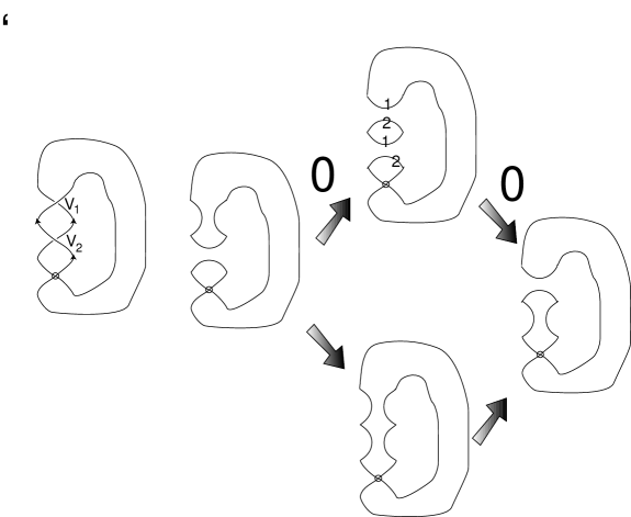
Figure 6: A face of the cube

For the lower composition, we have the identical zero map by definition. Substituting $X$ into the upper composition, we get $\pm X\wedge X$ at the first step and $0$ at the second step. Substituting $1$, we first get $1_{1}\wedge X_{2}+X_{1}\wedge 1_{2}$ here the index refers to the number of circle (the first circle is the big one), and the second index refers to the crossing number. While passing to the second crossing $V_{2}$ the circles change their roles: the first circle becomes the lower one, and the second circle becomes the upper one. Moreover, for the first circle we get a basis change: $X$ maps to $-X$. Thus we get $-X\wedge 1+1\wedge X$, which is taken to zero by the multiplication $m$.

The example above is in fact the key example of [Ma6]; it works without any changes when $h=0$ (because $t$ does not appear in the comultiplication of $1$ or in the multiplication of $1\wedge X$).

But in the case $h=0$ it does appear, and this would lead to the fact that the $1\to 1$-bifurcation should not be zero any more. We will in fact need to introduce a new variable being the square root of $h$.

On the other hand, $h$ itself should be treated in a special way so that the multiplication $m$ and comultiplication $\Delta$ behave nicely with respect to $1\mapsto 1,X\mapsto X$.

We shall consider this problem in a separate publication.

6.2.1 The ${\bf Z}_{2}$-case

We first consider the ${\bf Z}_{2}$-case solution given in [Ma3]. First note that there is no difference between $\wedge$ and $\otimes$, and we shall use the notation $\otimes$.

We set all $1\to 1$ type partial differentials to be zero.

Here will show how the square root of $h$ appears. Of course, in this case we shall not need exterior products and control the signs. Consider the basic ring of coefficients ${\bf Z}_{2}[t,c]$ with $\deg t=4,\deg c=1$ (we assume $c^{2}=h$). Now, consider Fig. 6. We have the following situation: in the lower composition we have two maps corresponding to $1\to 1$ bifurcations, thus the corresponding matrix should look like $I\cdot I$; in the upper part we have the composition of two matrices $\Delta$ and then $\mu$. Starting with $1$, we get $\Delta(1)=1\otimes X+X\otimes 1+h1\times 1$. Multiplying, we see that $X\otimes 1$ and $1\otimes X$ cancel each other, and the only remaining term is $h\cdot 1$. Now, if we start with $X$, we get $X\to X\otimes X+t\cdot 1\otimes 1$. After the multiplication, we get $hX+t+t=h\cdot X$ (we are dealing with the ${\bf Z}_{2}$ case). Now we see that the corresponding transformation matrix looks like

$$\left(\begin{array}[]{c}1\\ X\end{array}\right)\mapsto\left(\begin{array}[]{cc}h&0\\ 0&h\end{array}\right)\cdot\left(\begin{array}[]{c}1\\ X\end{array}\right)$$ (11)

For this scalar matrix $h\cdot Id$ we set the bifurcation corresponding to the $1\to 1$-mapping to be $c\cdot Id$, and then any face of the bifurcation cube corresponding to Fig. 6 will (anti)commute. Then it is not difficult to see (see [Ma3]) that with this scalar $1\to 1$-bifurcation matrix, all other faces (anti)commute as well.

Now, the dotted gradings $gr$ appear straigthforwardly by counting monomials in $t$ and $c$ and correcting $gr^{\prime}$ by using this monomials. Denote the obtained homology by $Kh(K)_{tc}$.

Note that the degree of $c$ is $1$, so we will have half-integer gradings. This immeadiately leads to the following

Theorem 10.

If $Kh(K)_{tc}$ has a non trivial homology of half-integer additional grading then $K$ has no diagram with orientable corresponding atom. In particular, the knot $K$ is not classical.

6.2.2 The general case

Now we turn to the general case of the ring ${\bf Z}$, and we have to handle the faces of the cube corresponding to Fig. 6.

7 Gradings or filtrations? The spectral sequence

Since the works of Lee [Lee] and Rasmussen [Ras], spectral sequences play a significant role in knot homology. Sometimes it turns out that studying convergence of a spectral sequence leads to some interesting and deep invariants such as Rasmussen’s invariant, which is applicable to estimating the Seifert genus and the $4$-ball genus of classical links.

The Lee-Rasmussen spectral sequence starts with the Khovanov homology and ends up with some two-term homology which carries a nice information.

Recently (see [BN3]), it was discovered that the spectral sequence of Lee-Rasmussen does not converge after $E_{3}$-term, and that there are some nice torsions in Khovanov homology which survive after the $E_{3}$-term of the spectral sequence.

Our goal here is to construct a spectral sequence from the “complicated” theory with new dotted gradings to the “simple” (Khovanov) theory. Thus, in some sense our spectral sequence will behave with respect to the usual Khovanov homology as Khovanov homology itself behaves with respect to the Rasmussen homology.

It would also be very interesting to inspect two spectral sequences converging from the “complicated” theory to the Rasmussen theory.

The argument of the present section is standard. In all cases described above when we deal with one new (dotted) grading, the old differential $\partial=\partial^{\prime}+\partial^{\prime\prime}$ in the complex $[[K]]_{g}$ does not decrease the new grading.

Thus, let us introduce the (dotted) filtration on the chain spaces as follows: we set $[[K]]_{g}^{n}=\{c\in[[K]]_{g}|gr(c)\geq n\}$. Then we have $[[K]]_{g}^{\infty}\subset\dots[[K]]_{g}^{2}\subset[[K]]_{g}^{1}\subset[[K]]_{g}^{0}\subset[[K]]_{g}^{-1}\subset\dots\subset[[K]]_{g}^{-\infty}$.

The usual differential $\partial$ respects this filtration. This leads to the following

Theorem 11.

For any field of coefficients, there is a spectral sequence whose $E_{1}$-term is isomorphic to $[[K]]$ with the first differential $\partial$, the $E_{2}$-term isomorphic to the usual Khovanov comology, so that this spectral sequence converges to the homology of $[[K]]_{g}$ with respect to $\partial^{\prime}$.

The argument proving this theorem is standard. We also conjecture that all terms of this spectral sequence are invariants (of knots, braids, tangles) in the corresponding category.

It would be very interesting to know whether some terms of the spectral sequence described above survive after the braid stabilsations. In this case we would be able to hope to construct gradings for usual knots without going into the long category.

Returning to the Lee-Rasmussen theory, we see that in the dotted case, we have two complexes: the usual Khovanov complex and the complex $([[K]]_{LR},\partial_{LR})$ with homology $H(K)_{LR}$. They coincide in the case when we have no dotting, but they differ in the case when we have dotting.

Quite in the usual manner one proves

Theorem 12.

For the field ${\bf Q}$, there is a spectral sequence whose $E_{1}$-term is isomorphic to $[[K]]_{LR}$ with the first differential $\partial_{LR}$, the $E_{2}$-term isomorphic to the homology $H(K)_{LR}$, so that this spectral sequence converges to the Lee-Rasmussen homology.

Thus, two bigraded homology theories (the usual Khovanov theory with height and quantum grading) and the one described above (with height and dotted grading) both converge to the Lee-Rasmussen theory.

It is known that the Lee-Rasmussen theory give nice invariants (quantum gradings of the two surviving elements). It would be interesting to compare the convergence of the spectral sequence describing above: what is the meaning of the dotted grading of surviving elements?

8 Applications

The theory above has some obvious applications coming from the definitions. Thus, if we work for knots in thickened surfaces, there is a natural question whether such a knot can be destablised, i.e., some handles of the surface are nugatory, or, in other words, the representative of the knot given by this surface is minimal. The surface $M$ has ${\bf Z}_{2}$-homology group of rank $k$, and if they are all used as gradings of some homology groups of a knot in $M\tilde{\times}I$, then the knot can not be destabilised.

Corollary 1.

If a set of additional gradings of non-trivial groups of $Kh_{gg}(K)$ forms a subset in ${\bf R}^{k}$ not belonging to any hypersurface passing through zero, then the link $K$ does not admit destabilisation, i.e., there is no surface $M^{\prime}$ of smaller genus obtained from $M$ by a destabilisation so that the link $K$ lies in the natural fibration over $M^{\prime}$ generated by ${\cal M}\to M$.

Analogously, the dotted grading can be used for estimating the number of virtual crossings of a rigid virtual knot diagram.

Also, we mention (without any details, however) the facts which generalise straightforwardly for the case of new gradings:

1. The homological length of the complex does not exceed the number of classical crossings.

2. The spanning tree of Wehrli [Weh] and Champanerkar-Kofman [ChK] saying that the Khovanov homology can be obtained from a complex with a smaller chain group. This leads to the estimation for the thickness:

   $Th(Kh(K))\leq 2+g$, where $g$ is the genus of the atom corresponding to the diagram $K$.

   Here the thickness estimates the number of diagonals with slope $2$ on the plane with height and quantum gradings serving as coordinates.

   The same estimates can be obtained for our complex with new gradings when looking at the diagonals with respect to the former gradings. This leads to

   Theorem 13.

   For any knot $K$, the thickness of the dotted Khovanov homology $Th(Kh(K))\leq 2+g$, where $g$ is the genus of the atom.

   Together with the lemma saying that $span\langle K\rangle\leq 4n$, where $n$ is the number of classical crossings, we get sharper estimates for the number of crossings.

3. The Bar-Natan topological picture [BN2] for tangles and cobordisms, see also [TuTu]. We need to generalize Bar-Natan’s topological category and construct a functor from it to our category. We shall discuss this in a separate publication.

4. Rasmussen’s estimates for the genus of a spanning surface; here we must, indicate the category of cobordisms, say, for knots in $M\times I$ we should consider spanning surfaces in $M\times I\times I$.

9 The relation to other papers

This paper generalises many constructions. First of all, we would like to mention the work [APS], the work [Kh2] and the work [Ma6].

In fact, the idea of taking new gradings counting $X$ and $1$ on non-trivial circles with opposite sides was originally used in [APS]. However, we used this approach for a more general situation. For instance, the grading there was necessary to construct the Khovanov homology itself; without it, the Khovanov theory for knots in thickened surfaces does not exist; even with it, it does not exist for knots in thickened ${\bf R}P^{2}$. We have taken the approach from [Ma6] with twisted coefficient as the basement for our homology theory (that allows us to give a fair generalisation of Khovanov’s theory for virtual and twisted knots without any new gradings), and then introduced new gradings similar to those ones by M.Asaeda, J.Przytycki and A.Sikora.

They used integral homology or even homotopy classes to define the gradings. This was quite difficult for making it more algebraic.

We have axiomatized this approach taking the ${\bf Z}_{2}$-cohomology (or just dotting) making it applicable to many other situations.

References

- [APS] Asaeda, M., Przytycki, J., Sikora, A. (2004), Categorification of the Kauffman bracket skein module of I-bundles over surfaces, Algebraic and Geometric Topology, 4, No. 52, pp. 1177-1210.
- [BN] Bar–Natan, D. (2002), On Khovanov’s categorification of the Jones polynomial, Algebraic and Geometric Topology, 2(16), pp. 337–370.
- [BN2] Bar–Natan, D. (2004), Khovanov’s homology for tangles and cobordisms, arXiv:mat.GT0410495.
- [BN3] Bar-Natan, D. (2007), Fast Khovanov homology computations, Journal of Knot Theory and Its Ramifications, 16 (3), pp. 243-256.
- [Bou] Bourgoin, M. O., Twisted Link Theory, arxiv: math. GT0608233
- [ChK] Champanerkar, A., Kofman, I., Spanning trees and Khovanov homology, arxiv: math. GT0607510
- [Dro] Drobotukhina Yu.V. (1991), An Analogue of the Jones-Kauffman poynomial for links in and a generalisation of the Kauffman-Murasugi Theorem, Algebra and Analysis, 2(3), pp. 613-630.
- [DK2] Dye, H.A., Kauffman, L.H. (2004), Minimal Surface Representation of Virtual Knots and Links, arXiv:math. GT/0401035 v1.
- [F] Fomenko A. T. (1991), The theory of multidimensional integrable hamiltonian systems (with arbitrary many degrees of freedom). Molecular table of all integrable systems with two degrees of freedom, Adv. Sov. Math, 6, pp. 1-35.
- [FKM] Fenn, R.A, Kauffman, L.H, and Manturov, V.O. (2005), Virtual Knots: Unsolved Problems, Fundamenta Mathematicae, Proceedings of the Conference “Knots in Poland-2003”, 188.
- [GPV] Goussarov M., Polyak M., and Viro O.// Topology. 2000. V. 39. P. 1045–1068.
- [Jac] Jacobsson, M. (2002), An invariant of link cobordisms from Khovanov’s homology theory, arXiv:mat.GT0206303 v1.
- [JKS] Jaeger, F., Kauffman, L.H., and H. Saleur (1994), The Conway Polynomial in and Thickened Surfaces: A new Determinant Formulation, J. Combin. Theory. Ser. B., 61, pp. 237-259.
- [KaV] Kauffman L.H., Virtual knot theory, Eur. J. Combinatorics. 1999. V. 20, N. 7. P. 662-690.
- [Kaw] Kawamura, K/ Khovanov homology and the braid index of a knot,
- [Kh] Khovanov, M. (1997), A categorification of the Jones polynomial, Duke Math. J,101 (3), pp.359-426.
- [Kh2] Khovanov, M. (2004), Link homology and Frobenius extensions, Arxiv.Math:GT/0411447
- [KhR1] Khovanov, M., Rozansky, L., Matrix Factorizations and Link Homology, Arxiv.Math:GT/0401268
- [KhR2] Khovanov, M., Rozansky, L.,Matrix Factorizations and Link Homology II, Arxiv.Math:GT/0505056
- [KK] Kamada, N. and Kamada, S. (2000), Abstract link diagrams and virtual knots, Journal of Knot Theory and Its Ramifications, 9 (1), pp. 93–109.
- [Kup] Kuperberg, G. (2002), What is a Virtual Link?, www.arXiv.org, math-GT0208039, Algebraic and Geometric Topology, 2003, 3, 587-591.
- [Lee] Lee, E.S. (2003) On Khovanov invariant for alternating links, arXiv: math.GT0210213.
- [ ] anturov, V.O., Teoriya Uzlov (Knot Theory, In Russian), RCD, M.-Izhevsk, 2005.
- [Ma1] Manturov, V.O. (2004), The Khovanov polynomial for Virtual Knots, Russ. Acad. Sci. Doklady, 398, N. 1., pp. 11-15.
- [Ma2] Manturov V.O. (2006), The Khovanov Complex and Minimal Knot diagrams, Russ. Acad. Sci. Doklady, 406, (3), pp. 308-311.
- [Ma3] Manturov V.O. (2005), The Khovanov complex for virtual knots, Fundamental and applied mathematics, 11, N. 4., pp. 127-152 (in Russian).
- [ 4] Manturov V.O. (2005), On Long Virtual Knots, Russ. Acad. Sci. Doklady, 401 (5), pp. 595-598.
- [Ma6] Manturov V.O. (2007), Khovanov Homology for Virtual Knots with Arbitrary Coefficients, Russ. Acad. Sci. Izvestiya, 71, N. 5, pp. 111-148.
- [Ma7] Manturov V.O. (2007) Additional gradings in the Khovanov Complex for Thickened Surfaces, Russ. Acad. Sci. Doklady, to appear.
- [Ma8] Manturov, V.O., Minimal diagrams of classical knots, ArXiv:GT/ 0501510.
- [Ma9] Manturov, V.O. (2003), Kauffman–like polynomial and curves in –surfaces, Journal of Knot Theory and Its Ramifications, 12, (8), pp.1145-1153.
- [Miy] Miyazawa, Y. (2006), Magnetic Graphs and an Invariant for Virtual Links, J. Knot Theory & Ramifications, 15 (10), pp. 1319-1334.
- [Oht] Ohtsuki, T. (2002), Quantum Invariants, World Scientific, Singapore.
- [Ras] Rasmussen, J. A. (2004), Khovanov Homology and the slice genus,ArXivMath:/GT. O402131.
- [Ras2] Rasmussen, J., Some Differentials on Khovanov-Rozansky Homology (2006), arXiv: math. GT0607544
- [Shu] Shumakovitch, A.//www.arxiv.org/math-gt/ 0405474.
- [TuTu] Turaev, V.G., Turner, P.(2005), Link homology and unoriented topological quantum field theory, //www.arxiv.org/math-gt/0506229 v1.
- [Viro] Viro, O., Virtual links and orientations of chord diagrams, Proceedings of the Gökova Conference-2005, International Press, pp. 187-212.
- [Weh] Wehrli, S.,A spanning tree model for Khovanov homology, arxiv: math. GT0409328