Superfluid Fermi-Fermi mixture: phase diagram, stability, and soliton formation

Abstract

We study the phase diagram for a dilute Bardeen-Cooper-Schrieffer superfluid Fermi-Fermi mixture (of distinct mass) at zero temperature using energy densities for the superfluid fermions in one (1D), two (2D), and three (3D) dimensions. We also derive the dynamical time-dependent nonlinear Euler-Lagrange equation satisfied by the mixture in one dimension using this energy density. We obtain the linear stability conditions for the mixture in terms of fermion densities of the components and the interspecies Fermi-Fermi interaction. In equilibrium there are two possibilities. The first is that of a uniform mixture of the two components, the second is that of two pure phases of two components without any overlap between them. In addition, a mixed and a pure phase, impossible in 1D and 2D, can be created in 3D. We also obtain the conditions under which the uniform mixture is stable from an energetic consideration. The same conditions are obtained from a modulational instability analysis of the dynamical equations in 1D. Finally, the 1D dynamical equations for the system are solved numerically and by variational approximation (VA) to study the bright solitons of the system for attractive interspecies Fermi-Fermi interaction in 1D. The VA is found to yield good agreement to the numerical result for the density profile and chemical potential of the bright solitons. The bright solitons are demonstrated to be dynamically stable. The experimental realization of these Fermi-Fermi bright solitons seems possible with present setups.

I Introduction

After the experimental realization of a trapped Bose-Einstein condensate (BEC) books there has been a great effort to trap and cool the Fermi atoms to degeneracy by sympathetic cooling in the presence of a second Bose or Fermi component. The second component is needed to facilitate evaporative cooling not possible due to lack of interaction in a single-component Fermi gas exp1 ; exp2 . Apart from the observation of the degenerate Bose-Fermi mixtures ^6,7Li exp3 ; mix-ex , ²³Na-⁶Li exp4 and ⁸⁷Rb-⁴⁰K exp5 ; exp5x , there have been studies of the following spin-polarized degenerate Fermi-Fermi mixtures ⁴⁰K-⁴⁰K exp1 and ⁶Li-⁶Li exp2 in different hyperfine states.

Specially challenging has been the experimental realization of vortex lattice in a Bardeen-Cooper-Schrieffer (BCS) superfluid Fermi gas exp6 ; exp7 ; bcsexp ; fw in Bose-Fermi mixture employing a weak attractive interaction among the intra-species fermions by using a Feshbach resonance fesh ; FESH . This attractive interaction allows the formation of BCS pairs leading to a BCS superfluid fw ; leggett-book . In the last few years by further increasing this attraction several experimental groups have observed the crossover cross from the paired BCS state to the BEC of molecular dimers with ultra-cold two-hyperfine-component Fermi vapors of ⁴⁰K greiner and ⁶Li atoms zwierlein ; chin . Another possibility is to use two distinct Fermi atoms for this purpose as suggested in Ref. skac in a study of collapse in a Fermi-Fermi mixture (⁶Li-⁴⁰K is a possible candidate for future exploration.) The Feshbach-resonance management of the Fermi interaction could be utilized to study a superfluid Fermi-Fermi mixture in a controlled fashion fesh .

In Bose-Fermi mixtures, there have been several studies on phase separation molmer ; pethick ; viverit ; das ; sala-toigo , soliton-like structures Sadhan-BFsoliton , and collapse skac2 , recently. The phase diagram of the Bose-Fermi mixture in three dimensions (3D) has been studied by Viverit et al. viverit , whereas the same in one dimension (1D) has been studied by Das das . Bright solitons have been observed in BECs of Li Li-soliton and Rb Rb-soliton atoms and studied subsequently BECsolitons . It has been demonstrated using microscopic BFsoliton(BBrepBFattr) and mean-field hydrodynamic Sadhan-BFsoliton models that the formation of stable fermionic bright solitons is possible in a degenerate Bose-Fermi mixture in the presence of a sufficiently attractive interspecies interaction which can overcome the Pauli-blocking repulsion among fermions. The formation of a soliton in these cases is related to the fact that the system can lower its energy by forming high density region (bright soliton) when the interspecies attraction is large enough to overcome the Pauli-blocking interaction in the degenerate Fermi gas (and any possible repulsion in the BEC) skbs . There have also been studies of mixing-demixing transition in degenerate Bose-Fermi sala-sadhan2 and Fermi-Fermi skabm mixtures, and soliton formation in Fermi-Fermi mixtures ff .

In this paper we investigate the phase diagram of a BCS superfluid Fermi-Fermi mixture of fermion components of distinct mass at zero temperature using energy densities for the superfluid Fermi components in one, two (2D), and three dimensions. We derive the conditions of stability of the mixture in terms of the densities of the components and the strength of interspecies interaction. The two possible phases of the mixture are a uniformly mixed configuration and a totally separated pure-phase configuration. Unlike in a Bose-Fermi mixture viverit ; das , no complicated mixed phases are allowed in a superfluid Fermi-Fermi mixture in 1D and 2D. However, a mixed and a pure phase is allowed in 3D. In 1D, two pure and separated phases of the fermion components appear for low fermion densities, whereas the opposite is found in 3D. In 1D, a uniform mixture appears for large fermion densities with the opposite taking place in 3D. In 2D, the condition for uniform mixture and phase separation is independent of density of the components. In 1D, we find the uniform mixture to be unstable for small fermion densities, whereas In 3D, the uniform mixture is unstable for large fermion densities.

The 1D configuration is of special interest due to soliton formation by modulational instability of a uniform mixture. To study this phenomenon we derive a set of dynamical equations of the system as the Euler-Lagrange equation of an appropriate Lagrangian. The condition of stability of the uniform mixture and the formation of soliton for attractive interspecies Fermi-Fermi interaction were studied from an energetic consideration as well as with a linear stability analysis of the constant-amplitude solution of the above dynamical equations. We solved the 1D dynamical equations numerically and variationally to study some features of the bright solitons. The numerical results for the density of the fermion components as well as their chemical potentials are found to be in good agreement with the variational findings. These bright solitons are found to be stable numerically when they are subjected to a perturbation.

The dependence of Fermi energy densities in 1D and 2D on atomic densities has counterparts in Bose systems and the analysis presented here is also applicable to these Bose systems. The 2D Fermi energy density has a quadratic dependence on atomic density as in a dilute BEC obeying the Gross-Pitaevskii equation, thus allowing the present results to be applicable to such a BEC books . The 1D Fermi energy density, on the other hand, has a cubic dependence on atomic density as in a Tonks-Girardeau Tonks (TG) Bose gas observed recently tg , thus making the present results applicable to this system.

The paper is organized as follows. In Sec. II we consider the stability condition of a uniform BCS superfluid Fermi-Fermi mixture from an energetic consideration. In Sec. III we consider a two-phase BCS superfluid Fermi-Fermi mixture in 1D, 2D and 3D and study the possibility of the formation of two phases from a consideration of pressure, energy and chemical potential of the system. We can have two pure phases or a uniformly mixed phase in all dimensions. In addition, in 3D, we can have a pure and a mixed phase. In Sec. IV we consider the Euler-Lagrange nonlinear dynamical equations for the system in 1D and study the modulational instability of the constant-amplitude solution representing the uniform mixture. The condition of modulational instability for attractive Fermi-Fermi interaction is found to be consistent with the condition of stability of the uniform mixture obtained from an energetic consideration in Sec. II. We further solve these dynamical equations numerically and variationally to analyze the properties of the Fermi-Fermi solitons. Finally, in Sec. V we present a summary of our study.

II Uniform Superfluid Fermi-Fermi Mixture

II.1 Energy Density of a Component

We consider a single-component dilute BCS superfluid of spin-half Fermi atoms of mass $m$ and density $n_{3}$ with a weak attraction between fermions with opposite spin orientations. In 3D, the energy density of this system is given by yang1 ; yang2 ; heis ; salasnich ,

$$\mathcal{E}_{\mathrm{3D}}=(3/5){n}_{\mathrm{3}}\varepsilon_{F}$$ (1)

where $\varepsilon_{F}=\left(\hbar k_{F}\right)^{2}/(2m)$ is the Fermi energy, $\hbar k_{F}$ is the Fermi momentum (this expression was first obtained by Lee and Yang yang2 in the weak-coupling BCS limit). Modifications to this expression for a description of the BCS-BEC crossover, for stronger attraction between fermions, have also been considered salasnich . The total density of the fermions in a 3D box is obtained by filling the quantum states up to the Fermi energy and is given by ${n}_{\mathrm{3}}={2(2\pi)^{-3}}\int_{0}^{k_{F}}4\pi k^{2}dk\equiv\left(3\pi^{2}\right)^{-1}\left(2m\varepsilon_{F}/\hbar^{2}\right)^{3/2}$. (The factor of 2 in the expression for $n_{3}$ accounts for BCS pairing in each level.) Hence the energy density in (1) becomes

$$\mathcal{E}_{\mathrm{3D}}=\frac{3(3\pi^{2})^{2/3}\hbar^{2}}{10m}{n}_{3}^{5/3}=\frac{3}{5}A_{\mathrm{3}}{n}_{3}^{5/3},$$ (2)

with $A_{\mathrm{3}}=\hbar^{2}(3\pi^{2})^{2/3}/(2m)$.

Similarly, the energy density of a dilute 1D superfluid of atom density $n_{1}$ is given by yang3 ; recati

$$\mathcal{E}_{\mathrm{1D}}=(1/3)n_{\mathrm{1}}\varepsilon_{F}.$$ (3)

This was obtained using the Gaudin-Yang (GY) model yang3 of fermions weakly interacting via zero-range ($\delta$-function) potential, and was later extended to the description of the BCS-to-unitarity crossover recati . (For repulsive interaction the GY model gives xt a Tomonaga-Luttinger liquid TL , while for attractive interaction it leads to a Luther-Emery liquid LE . For weak attraction the ground state of the system is a BCS superfluid fw ; KO . With the increase of attraction, the strong-coupling regime of tightly bound dimers is attained, which behaves like a hard core Bose gas, or like a 1D noninteracting Fermi gas, known as the TG gas Tonks ; ad-sa .) The general solution for the ground-state energy in the GY model has been obtained by solving the Bethe ansatz bethe equations for all strengths of $\delta$ interaction connecting the weak-attraction regime of BCS condensate to the strong-attraction regime of of tightly bound dimers described by the Lieb-Liniger model ll of repulsive bosons. This solution can be presented as an expansion series in limits of weak or strong interactions. The limiting value of this solution in the weak interaction BCS limit is given by Eq. (3) recati ; xt .

The fermion density of the BCS superfluid in a 1D box is $n_{\mathrm{1}}={2(2\pi)}^{-1}\int_{-k_{F}}^{+k_{F}}dk\equiv\left(2/\pi\hbar\right)\sqrt{2m\varepsilon_{F}}$, hence, in this case, $\varepsilon_{F}=\pi^{2}\hbar^{2}n_{1}^{2}/(8m)$, and energy density (3) becomes recati2

$$\mathcal{E}_{\mathrm{1D}}=\frac{\pi^{2}\hbar^{2}}{24m}n_{\mathrm{1}}^{3}=\frac{1}{3}A_{\mathrm{1}}n_{\mathrm{1}}^{3},$$ (4)

with $A_{\mathrm{1}}=\hbar^{2}\pi^{2}/(8m)$. The energy density of a TG gas Tonks is given by $\mathcal{E}_{\mathrm{TG}}=\hbar^{2}\pi^{2}n_{1}^{3}/6m$ ad-sa and is very similar to that given by Eq. (4). The difference in numerical factors between the two expressions is due to pairing in the present Fermi superfluid allowing two fermions (spin up and down) in the same quantum level. Hence the 1D results of the present study is also applicable to a TG gas.

Finally, a counterpart of relations (1) and (4) for the 2D superfluid is luca2 $\mathcal{E}_{\mathrm{2D}}=(1/2)n_{\mathrm{2}}\varepsilon_{F}$, the 2D density being $n_{\mathrm{2}}={2(2\pi)^{-2}}\int_{0}^{k_{F}}2\pi kdk\equiv\left(m/\pi\hbar^{2}\right)\varepsilon_{F}$, with $\varepsilon_{F}=\pi\hbar^{2}n_{\mathrm{2}}/m$. Thus, the energy density of the 2D superfluid can be written as luca2

$$\mathcal{E}_{\mathrm{2D}}=\frac{\pi\hbar^{2}}{2m}n_{\mathrm{2}}^{2}=\frac{1}{2}A_{\mathrm{2}}n_{\mathrm{2}}^{2},$$ (5)

with $A_{\mathrm{2}}=\pi\hbar^{2}/m$.

Here we specify the criteria of applicability of Eqs. (2), (4), and (5) for different dimensionalities. These results are valid for a dilute BCS superfluid. In 3D, at low densities, $k_{F}|a_{F}|<<1$ with $a_{F}$ the Fermi-Fermi scattering length, gaps are small and have little effect on the total energy of the system heis . The total energy density of the ground state can then be expanded in powers of the small parameter $k_{F}|a_{F}|$. At low densities Eq. (2) includes the lowest order term in this expansion yang2 . The condition $k_{F}|a_{F}|<<1$ of validity of Eq. (2) can be related to the gas parameter $n_{3}|a_{F}|^{3}$ in 3D: $n_{3}|a_{F}|^{3}<<1/(3\pi^{2})$, as the density $n_{3}=k_{F}^{3}/(3\pi^{2})$. In 1D, for a $\delta$ interaction of strength $g_{1}$ the dimensionless coupling constant $\gamma=mg_{1}/(\hbar^{2}n_{1})$ and the condition of validity of Eq. (4) is $|\gamma|<<1$ recati . In two dimensions an attractive interaction leads to a bound state of energy $\epsilon_{0}$ and the condition of diluteness for the validity of Eq. (5) can be expressed as $\epsilon_{0}/\varepsilon_{F}<<1.$

II.2 Stability Condition of the Uniform Mixture

We consider a uniform mixture of two types of fermions, containing $N_{i},i=1,2$, atoms (of mass $m_{1}=m$ and $m_{2}=m/\lambda$) , in a box of size $S$ (in 1D the size is a length, in 2D an area, and in 3D a volume) with distinct mass at zero temperature. The energy density of the uniform mixture is given by

$${\cal E}_{\mathrm{1D}} = \frac{1}{3}A_{\mathrm{1}}n_{1(1)}^{3}+g_{12}\,n_{1}\,n_{2}+\frac{1}{3}\lambda A_{\mathrm{1}}n_{1(2)}^{3},$$ (6)

$${\cal E}_{\mathrm{2D}} = \frac{1}{2}A_{\mathrm{2}}n_{2(1)}^{2}+g_{12}\,n_{1}\,n_{2}+\frac{1}{2}\lambda A_{\mathrm{2}}n_{2(2)}^{2},$$ (7)

$${\cal E}_{\mathrm{3D}} = \frac{3}{5}A_{\mathrm{3}}n_{3(1)}^{5/3}+g_{12}\,n_{1}\,n_{2}+\frac{3}{5}\lambda A_{\mathrm{3}}n_{3(2)}^{5/3},$$ (8)

respectively, for 1D, 2D and 3D systems, where $n_{d(i)}=N_{i}/S$ denotes the density of each component in $d$D, $d=1,2,3$. The nonlinear terms involving $g_{12}=4\pi\hbar^{2}a_{12}/m_{12}$ in above equations represent the interaction between two types of atoms arising solely from the atomic scattering length $a_{12}$, where $m_{12}$ is the reduced mass of atoms. The terms involving $A_{j}$ in the above equations, although is similar to the $gn^{2}/2$ interaction term for bosons (with $g=4\pi\hbar^{2}a/m$ representing the self interaction of a dilute boson gas with $a$ the Bose-Bose scattering length and $m$ the mass of an atom), have a different origin as we have seen. These terms originating from the energy of the fermions occupying the lowest quantum levels at zero temperature obeying Pauli principle generate an effective repulsion between the fermions and is usually called Pauli-blocking interaction.

The chemical potentials $\mu_{i}\equiv\partial{\cal E}/\partial n_{i}$ for species $i=1,2$ in 1D, 2D and 3D, are given, respectively, by

$$\mu_{1} = A_{\mathrm{1}}n_{1(1)}^{2}+g_{12}n_{1(2)},\quad\mu_{2}=g_{12}n_{1(1)}+\lambda A_{\mathrm{1}}n_{1(2)}^{2},$$

$$\mu_{1} = A_{\mathrm{2}}n_{2(1)}+g_{12}n_{2(2)},\quad\mu_{2}=g_{12}n_{2(1)}+\lambda A_{\mathrm{2}}n_{2(2)},$$

$$\mu_{1} = A_{\mathrm{3}}n_{3(1)}^{2/3}+g_{12}n_{3(2)},\quad\mu_{2}=g_{12}n_{3(1)}+\lambda A_{\mathrm{3}}n_{3(2)}^{2/3}.$$

The uniformly mixed phase is energetically stable if its energy is a minimum with respect to small variations of the densities, while the total number of fermions and bosons are held fixed. The conditions of stability [are the conditions of a minimum of ${\cal E}(n_{(1)},n_{(2)})$ as a function of two variables $n_{(1)}$ and $n_{(2)}$ and] are given by

$$\frac{\partial^{2}{\cal E}}{\partial n_{(1)}^{2}}\equiv\frac{\partial\mu_{1}}{\partial n_{(1)}}\geq 0,\quad\frac{\partial^{2}{\cal E}}{\partial n_{(2)}^{2}}\equiv\frac{\partial\mu_{2}}{\partial n_{(2)}}\geq 0,$$ (12)

$$\frac{\partial^{2}{\cal E}}{\partial n_{(1)}^{2}}\frac{\partial^{2}{\cal E}}{\partial n_{(2)}^{2}}-\left(\frac{\partial^{2}{\cal E}}{\partial n_{(1)}\partial n_{(2)}}\right)^{2}\equiv\frac{\partial\mu_{1}}{\partial n_{(1)}}\frac{\partial\mu_{2}}{\partial n_{(2)}}-\frac{\partial\mu_{1}}{\partial n_{(2)}}\frac{\partial\mu_{2}}{\partial n_{(1)}}\geq 0,$$

where we have dropped the dimension suffix. The solution of these inequalities gives the region in the parameters’ space where the uniformly mixed phase is energetically stable. Using Eqs. (12) and (II.2) the condition of stability of the uniform mixture in 1D, 2D, and 3D are given, respectively, by viverit ; ad-sa

$$4A_{\mathrm{1}}^{2}\lambda n_{(1)}n_{(2)}\geq g_{12}^{2},$$ (14)

$$A_{\mathrm{2}}^{2}\lambda\geq g_{12}^{2},$$ (15)

$$4A_{\mathrm{3}}^{2}\lambda\geq 9g_{12}^{2}n_{(1)}^{1/3}n_{(2)}^{1/3}.$$ (16)

These conditions are determined by $g_{12}^{2}$ and not the sign of $g_{12}$.

In 1D, we find from Eq. (14) with a finite $g_{12}^{2}$, that at small fermionic densities (small $n_{(1)}$ and $n_{(2)}$) the uniform mixture is unstable: the ground-state of the system displays demixing if $g_{12}>0$ and becomes a localized Fermi-Fermi bright soliton if $g_{12}<0$ ad-sa . The mixture is stable at large fermionic densities. In 2D, Eq. (15) reveals that the condition for stability is independent of density. In 3D, Eq. (16) predicts that for a finite $g_{12}^{2}$, the mixture is unstable at large fermionic densities, leading to collapse for $g_{12}<0$ and to demixing for $g_{12}>0$, and stable at small fermionic densities. It is realized that as we move from 1D to 3D through 2D, the condition of stability of the uniform mixture changes from large fermion densities to small fermion densities. This result is quite similar to that in a Bose-Fermi mixture viverit ; das , where the condition of stability of the uniform mixture is independent of the bosonic density and has a similar dependence on fermion density, e.g., during the passage from 1D to 3D through 2D, the condition of stability changes from large fermion density to small fermion density.

From inequality (12) the stability condition of a single component uniform gas can be represented as $\partial\mu_{1}/\partial n_{1}>0$, which, using Eqs. (II.2), (II.2) and (II.2), is realized for $A_{d}>0$ denoting a repulsive system. In the presence of a second component, inequality (II.2) can be written as viverit

$$\frac{\partial\mu_{1}}{\partial n_{(1)}}-\left(\frac{\partial\mu_{2}}{\partial n_{(1)}}\right)^{2}\frac{\partial n_{(2)}}{\partial\mu_{2}}\geq 0,$$ (17)

as ${\partial\mu_{2}}/{\partial n_{(1)}}={\partial\mu_{1}}/{\partial n_{(2)}}$. The first term ${\partial\mu_{1}}/{\partial n_{(1)}}$ in inequality (17) represents the effective repulsion among fermions of type 1. The second term, representing an induced interaction due to the presence of component 2, reduces the repulsion and tries to destabilize the uniform mixture. The uniform mixture becomes unstable when the second term in inequality (17) becomes larger than the first term. This happens for both attractive and repulsive interspecies interaction $g_{12}={\partial\mu_{2}}/{\partial n_{(1)}}$.

The inequality (II.2) can be written as

$$c_{1}^{2}c_{2}^{2}\geq 4g_{12}^{2}n_{(1)}n_{(2)},$$ (18)

where $c_{i}=\sqrt{2n_{(i)}(\partial\mu_{i}/\partial n_{(i)})}$ represent sound velocities in the two superfluid components, $i=1,2$. The sound velocity $c_{12}$ of the 1D Fermi-Fermi mixture can be obtained following a procedure suggested by Alexandrov and Kabanov kabanov ; ad-sa for a two-component BEC:

$$c_{12}={\frac{1}{\sqrt{2}}}\sqrt{c_{1}^{2}+c_{2}^{2}\pm\sqrt{(c_{1}^{2}-c_{2}^{2})^{2}+16g_{12}^{2}n_{(1)}n_{(2)}}}\;.$$ (19)

The homogeneous mixture becomes unstable when the sound velocity $c_{12}$ becomes imaginary, e.g., when inequality (18) is violated.

III Two-Phase Superfluid Fermi-Fermi Mixture

In the last section we considered a uniform mixture of two components in equilibrium. Here we explore the more interesting case of two types of fermions with different possible densities in different regions of a box of size $S.$ The components may mix uniformly or form separate phases depending on the initial conditions $-$ mass, density, interspecies interaction etc.

The conservation of the number of particles, $N_{1}$ and $N_{2}$, of the two species can be expressed as viverit ; das

$$N_{i}=Sn_{i}={S}\sum_{j=1}^{2}n_{i,j}f_{j},\quad\sum_{j=1}^{2}f_{j}=1,$$ (20)

where $i=1,2$ represent the species and $j=1,2$ represent the phases (different region with distinct density of gas), $n_{i}=N_{i}/S$ represent the overall density of the two species, $n_{i,j}$ is the density of species $i$ in phase $j$, and $S_{j}=Sf_{j}$ represent the size of each phase with $f_{j}$ the fraction of size in phase $j$. For a two-component system one can have only two distinct phases, $j=1,2$, as the inclusion of more phases leads to inconsistency viverit . Here we have dropped the dimension label $d$ and also removed the parentheses () from the component label $i$.

The total energy of the system is given by

$${E} = \sum_{j=1}^{2}{E}_{j}\equiv S\sum_{j=1}^{2}f_{j}{\cal E}_{j}$$ (21)

where ${\cal E}_{j}$ denotes the energy density of phase $j$ and ${E}_{j}$ its total energy. The pressure $P_{j}$ of phase $j$ is given by $P_{j}=-\partial{E}_{j}/\partial S_{j}$. The chemical potential of component $i$ in phase $j$ is defined by $\mu_{i,j}=\partial{\cal E}_{j}/\partial n_{i,j}$.

For equilibrium, the pressure in one phase has to be equal to that in the other. If two phases are occupied by atoms of the same type, the chemical potential for that type of atoms in two phases should also be equal so that the equilibrium can be energetically maintained. If the atom density of one type of atom in a phase is zero then the chemical potential of that type of atom in this phase should be larger than that in the other, so that the atoms do not flow to the phase with no atoms of this type viverit .

In the following we consider a system composed of two phases comprising of fractions $f_{1}=f$ and $f_{2}=(1-f)$ of size $S$. There are three following possibilities to be analyzed in 1D, 2D, and 3D, although some of them may not materialize in a particular case:

(i) Two pure and separated phases with one type of atom occupying a distinct phase.

(ii) A mixed and a pure phase where the density of one type of atoms is zero in one phase.

(iii) Two mixed phases where both phases are occupied by both type of atoms.

In the following we deal with the three possibilities in 1D, 2D and 3D. First, we consider the 2D case as the algebra is significantly simpler in this case.

III.1 Two-Dimensional (2D) Mixture

From Eqs. (7) we find that the expressions for total energy and pressure in this case are

$${E}_{j} = S_{j}{\cal E}_{j}\equiv S_{j}\left[\frac{1}{2}A_{\mathrm{2}}(n_{1,j}^{2}+\lambda n_{2,j}^{2})+g_{12}n_{1,j}n_{2,j}\right],$$ (22)

$$P_{j} \equiv -\frac{\partial{E}_{j}}{\partial S_{j}}=\frac{1}{2}A_{\mathrm{2}}n_{1,j}^{2}+g_{12}n_{1,j}n_{2,j}+\frac{1}{2}A_{\mathrm{2}}\lambda n_{2,j}^{2}.$$ (23)

In deriving Eq. (23) we recall that $n_{i,j}\sim 1/S_{j}$. From Eq. (22) the chemical potentials are given by

$$\mu_{1,j} = A_{\mathrm{2}}n_{1,j}+g_{12}n_{2,j}$$ (24)

$$\mu_{2,j} = A_{\mathrm{2}}\lambda n_{2,j}+g_{12}n_{1,j}$$ (25)

III.1.1 Two Pure Phases

In case of two pure and separated phases one should have, for example $n_{1,2}=n_{2,1}=0$ corresponding to the type one atoms occupying phase 1 only ($n_{1,1}\neq 0$) and type 2 atoms occupying phase 2 only ($n_{2,2}\neq 0$).

Equality of pressure $P_{1}=P_{2}$ in the two phases yields

$$n_{1,1}^{2}=\lambda n_{2,2}^{2}.$$ (26)

As the number of atoms is zero in one of the phases, one has the inequalities $\mu_{2,2}\leq\mu_{2,1}$ and $\mu_{1,1}\leq\mu_{1,2}$ on the chemical potential, which, using Eqs. (24) and (25), become

$$A_{\mathrm{2}}\lambda n_{2,2} \leq g_{12}n_{1,1},$$ (27)

$$A_{\mathrm{2}}n_{1,1} \leq g_{12}n_{2,2}.$$ (28)

Eliminating $n_{1,1}$ and $n_{2,2}$ among Eqs. (26), (27), and (28) we get

$$A_{\mathrm{2}}^{2}\lambda\leq g_{12}^{2},$$ (29)

consistent with inequality (15). We have the uniform mixture for inequality (15); for the opposite inequality (29) we have the separated phases in equilibrium. These inequalities are independent of the atomic densities.

In the present case the overall densities of the two species are given by

$$n_{1}=f_{1}n_{1,1}=fn_{1,1},\quad n_{2}=f_{2}n_{2,2}=(1-f)n_{2,2}.$$ (30)

Let us now consolidate these findings using energetic considerations comparing the total energy of a phase-separated configuration with that of a uniform mixture. The energy of the mixture is given by

$${E}_{\mathrm{mix}} = S\left[\frac{1}{2}A_{\mathrm{2}}n_{1}^{2}+g_{12}n_{1}n_{2}+\frac{1}{2}A_{\mathrm{2}}\lambda n_{2}^{2}\right],$$

$$= S\biggr{[}\frac{1}{2}A_{\mathrm{2}}f^{2}n_{1,1}^{2}+g_{12}n_{1,1}n_{2,2}f(1-f)$$

$$+ \frac{1}{2}A_{\mathrm{2}}\lambda n_{2,2}^{2}(1-f)^{2}\biggr{]},$$ (32)

where we have used Eqs. (30). The energy of the phase-separated system with the same number of atoms is

$${E}_{\mathrm{sep}} = S\left[\frac{1}{2}A_{\mathrm{2}}fn_{1,1}^{2}+\frac{1}{2}A_{\mathrm{2}}\lambda(1-f)n_{2,2}^{2}\right].$$ (33)

Using Eq. (26), one has for the difference

$${E}_{\mathrm{mix}}-{E}_{\mathrm{sep}}=Sf(1-f)n_{2,2}^{2}\sqrt{\lambda}[g_{12}-A_{\mathrm{2}}\sqrt{\lambda}].$$ (34)

When ${E}_{\mathrm{mix}}>{E}_{\mathrm{sep}}$ the system naturally moves to the separated phase and this happens for $g_{12}^{2}>A_{\mathrm{2}}^{2}\lambda$, consistent with inequality (29), leading to a stable separated phase. In the opposite limit, when ${E}_{\mathrm{mix}}<{E}_{\mathrm{sep}}$, the energetic consideration favors the uniform mixture and this happens for $g_{12}^{2}<A_{\mathrm{2}}^{2}\lambda$, consistent with inequality (15).

III.1.2 A mixed and a pure phase

Here we consider one mixed phase (phase 1) and one pure phase (phase 2) consistent with $n_{1,2}=0$, which means that the type 1 atoms occupy only phase 1, whereas type 2 atoms occupy both phases 1 and 2. Using Eq. (23) the equality of pressure in two phases leads to

$$\frac{1}{2}A_{\mathrm{2}}n_{1,1}^{2}+g_{12}n_{1,1}n_{2,1}+\frac{1}{2}A_{\mathrm{2}}\lambda n_{2,1}^{2}=\frac{1}{2}A_{\mathrm{2}}\lambda n_{2,2}^{2}.$$ (35)

From Eq. (25) the equality of the chemical potential of type 2 atoms in two phases ($\mu_{2,2}=\mu_{2,1}$) leads to

$$n_{1,1}=A_{\mathrm{2}}\lambda(n_{2,2}-n_{2,1})/g_{12}.$$ (36)

From Eq. (24) the inequality of the chemical potential of type 1 atoms in two phases ($\mu_{1,1}<\mu_{1,2}$) leads to

$$A_{\mathrm{2}}n_{1,1}<g_{12}(n_{2,2}-n_{2,1}),$$ (37)

which using Eq. (36) yields

$$A_{\mathrm{2}}^{2}\lambda<g_{12}^{2}.$$ (38)

Substituting Eq. (36) into Eq. (35) and after some straightforward algebra we obtain

$$(A_{\mathrm{2}}^{2}\lambda-g_{12}^{2})(n_{2,1}-n_{2,2})^{2}=0,$$ (39)

which allows two possibilities. For $A_{\mathrm{2}}^{2}\lambda\neq g_{12}^{2}$, the only solution is the trivial, nevertheless unacceptable, one $n_{2,1}=n_{2,2}$, which means that the type 2 atoms form a uniform configuration and not a mixed phase. However, if $A_{\mathrm{2}}^{2}\lambda=g_{12}^{2}$, one can have a mixed phase with $n_{2,1}\neq n_{2,2}$. Nevertheless, this condition enters in contradiction with inequality (38), showing that one cannot have one mixed and one pure phase in this case.

Next we consider the possibility of two mixed phases. The equality of pressure and chemical potential of each species in two phases leads to the following conditions

$$\frac{1}{2}A_{\mathrm{2}}(n_{1,1}^{2}-n_{1,2}^{2}) + \frac{1}{2}A_{\mathrm{2}}\lambda(n_{2,1}^{2}-n_{2,2}^{2})$$ (40)

$$= g_{12}(n_{1,2}n_{2,2}-n_{1,1}n_{2,1}),$$

$$A_{\mathrm{2}}n_{1,1}+g_{12}n_{2,1} = A_{\mathrm{2}}n_{1,2}+g_{12}n_{2,2},$$ (41)

$$A_{\mathrm{2}}\lambda n_{2,1}+g_{12}n_{1,1} = A_{\mathrm{2}}\lambda n_{2,2}+g_{12}n_{1,2}.$$ (42)

This set of equations have only the trivial solutions $n_{1,1}=n_{1,2}$ and $n_{2,1}=n_{2,2}$ corresponding to uniform mixture. Hence two mixed phases cannot be in equilibrium.

III.2 One-Dimensional (1D) Mixture

From Eqs. (6), we find that the expression for total energy and pressure in this case are

$${E}_{j} = S_{j}{\cal E}_{j}\equiv S_{j}\left[\frac{1}{3}A_{\mathrm{1}}(n_{1,j}^{3}+\lambda n_{2,j}^{3})+g_{12}n_{1,j}n_{2,j}\right],$$

$$P_{j} \equiv -\frac{\partial{E}_{j}}{\partial S_{j}}=\frac{2}{3}A_{\mathrm{1}}n_{1,j}^{3}+g_{12}n_{1,j}n_{2,j}+\frac{2}{3}A_{\mathrm{1}}\lambda n_{2,j}^{3}.$$

From Eq. (22) the chemical potentials are given by

$$\mu_{1,j} = A_{\mathrm{1}}n_{1,j}^{2}+g_{12}n_{2,j}$$ (45)

$$\mu_{2,j} = A_{\mathrm{1}}\lambda n_{2,j}^{2}+g_{12}n_{1,j}.$$ (46)

III.2.1 Two pure phases

In case of two pure and separated phases one should have, for example, $n_{2,1}=0$ for phase 1 and $n_{1,2}=0$ for phase 2. The condition of equal pressure then yields

$$n_{1,1}^{3}=\lambda n_{2,2}^{3}.$$ (47)

For equal-mass fermions $\lambda=1$, and one obviously have have the trivial solution $n_{1,1}=n_{2,2}$ or the densities of the two species are equal. Of course, for $\lambda\neq 1$ the densities of the two species could be different. Chemical potential condition $\mu_{2,2}\leq\mu_{2,1}$ yields

$$A_{\mathrm{1}}\lambda n_{2,2}^{2}\leq g_{1,2}n_{1,1}.$$ (48)

Chemical potential condition $\mu_{1,1}\leq\mu_{1,2}$ yields

$$A_{\mathrm{1}}n_{1,1}^{2}\leq g_{1,2}n_{2,2}.$$ (49)

Eliminating $n_{1,1}$ between Eqs. (47) and (48) or between Eqs. (47) and (49) we get

$$n_{2,2}\leq B_{\mathrm{1}},\quad B_{\mathrm{1}}=g_{12}/(A_{1}\lambda^{2/3}).$$ (50)

From Eqs. (47) and (50) we obtain the following restriction on $n_{1,1}$

$$n_{1,1}\leq C_{\mathrm{1}},\quad C_{\mathrm{1}}=g_{12}/(A_{1}\lambda^{1/3}).$$ (51)

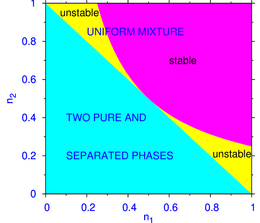
Figure 1: (Color online) Phase diagram for Fermi-Fermi mixture in one dimension (1D). The plotted density $n_{1}$ is in units of $C_{\mathrm{1}}\equiv g_{12}/(A_{\mathrm{1}}\lambda^{1/3})$ and $n_{2}$ in units of $B_{\mathrm{1}}\equiv g_{12}/(A_{\mathrm{1}}\lambda^{1/3}).$ The light gray area represents two pure and separated phases while the dark gray area represents the domain of stable uniform mixture. Below the curved line in the clear area the uniform mixture is unstable against small fluctuations.

In this case a phase diagram showing the total densities of type 1 and 2 fermions for which the system can completely separate, can be obtained from Eq. (30) if we allow $f$ to vary from 0 to 1 and use conditions (50) and (51). This is illustrated in Fig. 1. The light gray area represents pure phases and the dark gray area represents the stable uniform mixture. The uniform mixture is unstable in the clear area below the curve given by inequality (14). For attractive interaction, one has the formation of bright solitons by modulational instability, (discussed in Sec. IV). For repulsive interaction one can have a partially demixed configuration in the clear region in Fig. 1.

Now let us see if the system spontaneously move into the phase-separated configuration from an energetic consideration. The energy of the mixed system is

$${E}_{\mathrm{mix}} = S\left[\frac{1}{3}A_{\mathrm{1}}n_{1}^{3}+n_{1}n_{2}g_{12}+\frac{1}{3}\lambda A_{\mathrm{1}}n_{2}^{3}\right]$$

$$= S\biggr{[}\frac{1}{3}A_{\mathrm{1}}n_{1,1}^{3}f^{3}+n_{1,1}n_{2,2}f(1-f)g_{1,2}$$

$$+ \frac{1}{3}A_{\mathrm{1}}n_{2,2}^{3}(1-f)^{3}\lambda\biggr{]}.$$ (53)

Equation (53) is obtained with the use of Eq. (30). The energy of the separated phase system with the same number of atoms is

$${E}_{\mathrm{sep}}=\frac{1}{3}A_{\mathrm{1}}S[n_{1,1}^{3}f+n_{2,2}^{3}\lambda(1-f)].$$ (54)

Using Eq. (47), and after some straightforward algebra, the difference $\Delta\equiv({E}_{\mathrm{mix}}-{E}_{\mathrm{sep}})$ is given by

$$\Delta=n_{2,2}^{2}S\lambda^{1/3}[g_{12}-A_{\mathrm{1}}n_{2,2}\lambda^{2/3}]f(1-f)$$ (55)

Considering the restriction (50) in the separated phase, Eq. (55) yields the following inequality

$$\Delta=n_{2,2}^{2}f(1-f)S\lambda^{1/3}[1-n_{2,2}/B_{\mathrm{1}}]g_{12}\geq 0.$$ (56)

For density ranges where equilibrium is possible $f\neq 0$ and $f\neq 1$, $E_{\mathrm{sep}}$ is always less than $E_{\mathrm{mix}}$. Hence, energetically the two species of fermions can separate.

III.2.2 A mixed and a pure phase

Now let us consider a mixed phase (phase 1) and a pure phase (phase 2) and consider the case $n_{1,2}=0$. The equality of pressure now leads to

$$\frac{2}{3}A_{\mathrm{1}}n_{1,1}^{3}+\frac{2}{3}A_{\mathrm{1}}\lambda n_{2,1}^{3}+g_{12}n_{1,1}n_{2,1}=\frac{2}{3}A_{\mathrm{1}}\lambda n_{2,2}^{3}.$$ (57)

The equality of chemical potential of species 2 in two phases ($\mu_{2,1}=\mu_{2,2}$) yields

$$n_{1,1}=A_{\mathrm{1}}\lambda(n_{2,2}^{2}-n_{2,1}^{2})/g_{12}.$$ (58)

Eliminating $n_{1,1}$ between equations (57) and (58) (after some straightforward algebra) we get

$$2\Lambda(1-x^{2})^{3}=x^{3}-3x+2$$ (59)

where $x=n_{2,1}/n_{2,2}$, $\Lambda=(n_{2,2}/B_{\mathrm{1}})^{3}$. After cancelling the trivial factor $(1-x)^{2}$ from both sides of Eq. (59), we get

$$2\Lambda(1+x)^{3}(1-x)=x+2$$ (60)

From Eq. (60) we find that the solution $x=0$ is obtained for $\Lambda=1$ corresponding to $n_{2,1}=n_{1,2}=0$, $n_{2,2}=B_{\mathrm{1}}$ and $n_{1,1}=C_{\mathrm{1}}$. The densities of the first component are $n_{1,2}=0$ and $n_{1,1}=C_{\mathrm{1}}.$ This is the special case considered in Sec. IIIB1 [see, Eqs. (50) and (51)]. The solution $n_{2,2}=B_{\mathrm{1}}$ $(\Lambda=1)$ is a solution of two pure phases corresponding to $x=0$. The domain of solution of mixed phase corresponds to $n_{2,2}>B_{\mathrm{1}}$ $(\Lambda>1)$ corresponding to $x>0$ (recall that the fraction $x$ cannot be negative.) Hence for the present mixed phase to exist Eq. (60) should have the solution $x\to+0$ for $\Lambda\to+1$. However, we find from Eq. (60) as $\Lambda$ is made slightly greater than 1, the solution $x=0$ turns negative (unphysical). [Please note that for $\Lambda=1$ Eq. (60) has two real roots: $x=0,$ $0.7399...$; the latter (spurious) root is not of present physical interest.] Hence we conclude that a mixed and a pure phase cannot be realized in the present mixture.

Finally, one can consider the possibility of two mixed phases. The equality of pressure and chemical potential of each species in two phases leads to

$$\frac{2}{3}A_{\mathrm{1}}(n_{1,1}^{3}-n_{1,2}^{3}) + \frac{2}{3}A_{\mathrm{1}}\lambda(n_{2,1}^{3}-n_{2,2}^{3})$$ (61)

$$= g_{12}(n_{1,2}n_{2,2}-n_{1,1}n_{2,1}),$$

$$A_{\mathrm{1}}n_{1,1}^{2}+g_{12}n_{2,1} = A_{\mathrm{1}}n_{1,2}^{2}+g_{12}n_{2,2},$$ (62)

$$A\lambda n_{2,1}^{2}+g_{12}n_{1,1} = A\lambda n_{2,2}^{2}+g_{12}n_{1,2}.$$ (63)

This set of equations have only the trivial solutions $n_{1,1}=n_{1,2}$ and $n_{2,1}=n_{2,2}$ corresponding to uniform mixture and that is also possible when the condition of uniform mixture is satisfied. Hence two mixed phases cannot be in equilibrium.

III.3 Three-dimensional (3D) Mixture

From Eqs. (8), we find that the expression for total energy and pressure in this case are

$${E}_{j} = S_{j}{\cal E}_{j}\equiv S_{j}\left[\frac{3}{5}A_{\mathrm{3}}n_{1,j}^{5/3}+g_{12}n_{1,j}n_{2,j}+\frac{3}{5}A_{\mathrm{3}}\lambda n_{2,j}^{5/3}\right],$$

$$P_{j} \equiv -\frac{\partial{E}_{j}}{\partial S_{j}}=\frac{2}{5}A_{\mathrm{3}}n_{1,j}^{5/3}+g_{12}n_{1,j}n_{2,j}+\frac{2}{5}A_{\mathrm{3}}\lambda n_{2,j}^{5/3}.$$

From Eq. (22) the chemical potentials are given by

$$\mu_{1,j} = A_{\mathrm{3}}n_{1,j}^{2/3}+g_{12}n_{2,j}$$ (66)

$$\mu_{2,j} = A_{\mathrm{3}}\lambda n_{2,j}^{2/3}+g_{12}n_{1,j}.$$ (67)

III.3.1 Two pure phases

Again for two pure and separated phases we take $n_{1,2}=n_{2,1}=0$. The condition of equal pressure in two phases then leads to

$$n_{1,1}^{5/3}=\lambda n_{2,2}^{5/3}.$$ (68)

The chemical potential condition $\mu_{2,2}\leq\mu_{2,1}$ yields

$$n_{1,1}\geq\lambda A_{\mathrm{3}}n_{2,2}^{2/3}/g_{12}.$$ (69)

The chemical potential condition $\mu_{1,1}\leq\mu_{1,2}$ yields

$$n_{2,2}\geq A_{\mathrm{3}}n_{1,1}^{2/3}/g_{12}.$$ (70)

Eliminating $n_{1,1}$ between Eqs. (68) and (69) or between Eqs. (68) and (70) we obtain

$$n_{2,2}\geq B_{\mathrm{3}},\quad B_{\mathrm{3}}=(\lambda^{2/5}A_{3}/g_{12})^{3}.$$ (71)

Similarly, eliminating $n_{2,2}$ between Eqs. (68) and (69) we get

$$n_{1,1}\geq C_{\mathrm{3}},\quad C_{\mathrm{3}}=(\lambda^{3/5}A_{3}/g_{12})^{3}.$$ (72)

In this case a phase diagram showing the total densities of type 1 and 2 fermions for which the system can completely separate, can be obtained from Eq. (30) if we allow $f$ to vary from 0 to 1 and use conditions (71) and (72). This is illustrated in Fig. 2.

Figure 2: (Color online) Phase diagram for Fermi-Fermi mixture in three dimensions (3D). The plotted density $n_{1}$ is in units of $C_{\mathrm{3}}\equiv(\lambda^{2/5}A_{\mathrm{3}}/g_{12})^{3}$ and $n_{2}$ in units of $B_{\mathrm{3}}\equiv(\lambda^{3/5}A_{\mathrm{3}}/g_{12})^{3}.$ The light gray area represents two pure and separated phases while the dark gray area represents the domain of stable uniform mixture. The clear area represents the region where a mixed and a pure phase can exist. Above the curved line the uniform mixture is unstable against small fluctuations.

To see the separation of the two types of fermions from an energetic consideration, we calculate the energies of the mixed and separated configurations. The energy of the mixed phase is viverit

$${E}_{\mathrm{mix}} = S\left[\frac{3}{5}A_{\mathrm{3}}n_{1}^{5/3}+g_{12}n_{1}n_{2}+\frac{3}{5}A_{\mathrm{3}}\lambda n_{2}^{5/3}\right]$$

$$= S\biggr{[}\frac{3}{5}A_{\mathrm{3}}f^{5/3}n_{1,1}^{5/3}+g_{12}n_{1,1}n_{2,2}f(1-f)$$

$$+ \frac{3}{5}A_{\mathrm{3}}\lambda n_{2,2}^{5/3}(1-f)^{5/3}\biggr{]}.$$ (74)

The energy of the separated phase is

$${E}_{\mathrm{sep}} = S\left[\frac{3}{5}A_{\mathrm{3}}n_{11}^{5/3}f+\frac{3}{5}A_{\mathrm{3}}\lambda n_{2,2}^{5/3}(1-f)\right].$$ (75)

Using Eq. (68) the difference $\Delta=({\cal E}_{\mathrm{mix}}-{\cal E}_{\mathrm{sep}})$ can be written as

$$\Delta = S[3A_{3}\lambda n_{2,2}^{5/3}f(f^{2/3}-1)/5+g_{12}n_{22}^{2}\lambda^{3/5}f(1-f)$$ (76)

$$+ 3A_{\mathrm{3}}\lambda n_{2,2}^{5/3}(1-f)\{(1-f)^{2/3}-1\}/5].$$

Using inequality (70), Eq. (76) yields

$$\Delta \geq \frac{A_{\mathrm{3}}^{6}\lambda^{3}}{g_{12}^{5}}\biggr{[}-\frac{3}{5}f(1-f^{2/3})$$ (77)

$$+ f(1-f)-\frac{3}{5}(1-f)\{1-(1-f)^{2/3}\}\biggr{]}.$$

For $1>f>0$, the quantity given by (77) is always positive. Hence the separated phase has less energy than the mixed phase and the system will spontaneously move into the phase separated configuration.

In this case also two mixed phases cannot be in equilibrium as in 1D.

III.3.2 A mixed and a pure phase

Again we consider a mixed (species 2) and a pure (species 1) phase and consider the case $n_{1,2}=0$. The equality of pressure now leads to

$$\frac{2}{5}A_{\mathrm{3}}n_{1,1}^{5/3}+g_{12}n_{1,1}n_{2,1}+\frac{2}{5}A_{\mathrm{3}}\lambda n_{2,1}^{5/3}=\frac{2}{5}A_{\mathrm{3}}\lambda n_{2,2}^{5/3}.$$ (78)

The equality of chemical potential of species 2 in two phases ($\mu_{2,1}=\mu_{2,2}$) yields

$$n_{1,1}=A_{\mathrm{3}}\lambda(n_{2,2}^{2/3}-n_{2,1}^{2/3})/g_{12}.$$ (79)

Eliminating $n_{1,1}$ between Eqs. (78) and (79) and after some straightforward algebra we get

$$2\Lambda(1+x)^{5/3}-(1-x)^{1/3}(3x^{3}+6x^{2}+4x+2)=0,$$ (80)

where $x=(n_{2,1}/n_{2,2})^{1/3}$, and $\Lambda=(n_{2,2}/B_{\mathrm{3}})^{-5/9}$. From Eq. (80) we find that the solution $x=0$ is obtained for $\Lambda=1$ corresponding to $n_{2,1}=0$, $n_{2,2}=B_{\mathrm{3}}$, $n_{1,1}=C_{\mathrm{3}}$, $n_{1,2}=0$. This is the limiting case of two pure and separated phase studied in Sec. IIIC1. (In addition for $\Lambda=1$, Eq. (80) has the spurious or unphysical root $x=0.90278...$, which we do not consider here.) For two purely separated phases we have seen that $n_{2,2}\geq B_{\mathrm{3}}$ whence $\Lambda\equiv(n_{2,2}/B_{\mathrm{3}})^{-5/9}\leq 1.$ The domain for a mixed and a separated phase then should have $\Lambda>1$. To find this domain we solve Eq. (80) for $x>0$ using different $\Lambda$. Such solutions appear in the range $1.217...\geq\Lambda\geq 1$. Using this solution for $x$ we obtain $n_{2,2}$ and $n_{2,1}$ from the definitions of $\Lambda$ and $x$, respectively. Finally, $n_{1,1}$ is obtained from Eq. (79). The results so-obtained for $n_{2,2}$, $n_{2,1}$, and $n_{1,1}$ for different $\Lambda$ are used in

$$n_{1}=fn_{1,1},\quad\mbox{and}\quad n_{2}=fn_{2,1}+(1-f)n_{2,2},$$ (81)

to calculate the domain of $n_{1}$ and $n_{2}$, by varying $f$ in the range $1>f>0$, which allows a pure and a mixed phase.

We show the 3D phase diagram for total densities of type 1 and 2 fermions in Fig. 2. In this figure the light gray area represents the domain of two separated phases and the clear area that of a mixed and a separated phase as calculated above. The remaining dark gray area represents the domain of stable uniform mixture. The uniform mixture is unstable above the curve given by Eq. (16). Qualitatively, Fig. 2 is quite similar to Fig. 3 of Viverit et al. viverit for a Bose-Fermi mixture.

If we compare Figs. 1 and 2 we find that in 1D the pure phases appear at small densities, and uniform mixture at large densities. The uniform mixture is stable at larger densities. The opposite happens in 3D. If we compare the findings of Viverit et al. viverit for a study of the phase diagram of a Bose-Fermi mixture in 3D and compare with the study of Das das in 1D we find that such an inversion also takes place there. Moreover in 1D there cannot be a mixed and a pure phase for a Fermi-Fermi mixture, which is possible in 3D.

IV Dynamical Equations in Quasi-1D Superfluid Fermi-Fermi Mixture

IV.1 The Model

Of the three dimensional possibilities $-$ 1D, 2D and 3D $-$ the 1D case deserves special attention. In 1D, if the interspecies Fermi-Fermi interaction is attractive, in the domain of instability of the uniform mixture one can have the formation of bright soliton by modulational instability. To perform a careful study of the nature of these bright solitons (and their dynamical stability) we derive the Euler-Lagrange equations in 1D from its Lagrangian density.

We consider a mixture of $N_{1}$ superfluid atomic fermions of mass $m_{1}(=m)$ and $N_{2}$ superfluid atomic fermions of mass $m_{2}(=m/\lambda)$ at zero temperature trapped by a tight cylindrically symmetric harmonic potential of frequency $\omega_{\bot}$ in the transverse (radial cylindric) direction. We assume factorization of the transverse degrees of freedom. This is justified in 1D confinement where, regardless of the longitudinal behavior or statistics, the transverse spatial profile is that of the single-particle ground-state das ; sala-st ; sala-npse . The transverse width of the atom distribution is given by the characteristic harmonic length of the single-particle ground-state: $a_{\bot j}=\sqrt{\hbar/(m_{j}\omega_{\bot})}$, with $j=1,2$. The atoms have an effective 1D behavior at zero temperature if their chemical potentials are much smaller than the transverse energy $\hbar\omega_{\bot}$ das ; sala-st ; sala-npse . The interspecies Fermi-Fermi interaction is characterized by a contact potential with scattering length $a_{12}$, which can be repulsive or attractive.

We use a mean-field Lagrangian to study the static and collective properties of the 1D superfluid Fermi-Fermi mixture as in the Ginzburg-Landau theory fw . The Lagrangian density ${\cal L}$ of the mixture reads

$${\cal L}={\cal L}_{1}+{\cal L}_{2}+{\cal L}_{12}\;.$$ (82)

The term ${\cal L}_{i}$ is the fermionic Lagrangian for component $i$, defined as

$${\cal L}_{i}={i\hbar\over 2}\,\left(\psi_{i}^{*}{\partial\psi_{i}\over\partial t}-\psi_{i}{\partial\psi_{i}^{*}\over\partial t}\right)-{\hbar^{2}\over 2{m_{\mathrm{eff}}^{(i)}}}\left|{\partial\psi_{i}\over\partial z}\right|^{2}-\frac{A_{\mathrm{1}}^{(i)}}{3}|\psi_{i}|^{6},$$

(83)

where $A_{\mathrm{1}}^{(i)}=\hbar^{2}\pi^{2}/(8m_{i})$, $\psi_{i}(z,t)$ is the field of the $i$th component of the BCS Fermi superfluid along the longitudinal axis, such that $n_{i}(z,t)=|\psi_{i}(z,t)|^{2}$ is the 1D local probability density of the $i$th component. Here $m_{\mathrm{eff}}^{(i)}$ is the effective mass of superfluid flow in the Ginzburg-Landau theory. There is experimental evidence fw that this effective mass is twice the fermion mass ($m_{\mathrm{eff}}^{(i)}=2m_{i}$) and we shall use this effective mass in the following study.

Finally, the Lagrangian density ${\cal L}_{12}$ of the interaction between the two Fermi components is taken to be of the following standard zero-range form sala-st ; sala-sadhan2

$${\cal L}_{12}=-g_{12}\,|\psi_{1}|^{2}|\psi_{2}|^{2}\;,$$ (84)

where $g_{12}=2\hbar\omega_{\bot}a_{12}$ is the 1D Fermi-Fermi interaction strength.

The Euler-Lagrange equations of the Lagrangian ${\cal L}$ are the two following coupled partial differential equations:

$$i\hbar\partial_{t}\psi_{1} = \left[-\frac{\hbar^{2}}{4m_{1}}\partial_{z}^{2}+A_{\mathrm{1}}^{(1)}n_{1}^{2}+g_{12}n_{2}\right]\psi_{1}\;,$$ (85)

$$i\hbar\partial_{t}\psi_{2} = \left[-\frac{\hbar^{2}}{4m_{2}}\partial_{z}^{2}+A_{\mathrm{1}}^{(2)}n_{2}^{2}+g_{12}n_{1}\right]\psi_{2}\;,$$ (86)

with the normalization $\int_{-\infty}^{\infty}|\psi_{i}|^{2}dz=N_{i}$.

It is convenient to work in terms of dimensionless variables defined in terms of a frequency $\omega$ and length $l\equiv\sqrt{\hbar/(2m_{1}\omega)}$ by $\psi_{j}=\hat{\psi}_{j}/\sqrt{l}$, $t=2\hat{t}/\omega$, $z=\hat{z}l$, and $g_{12}={\hat{g}_{12}\hbar^{2}/(4m_{1}l)}$. With these new variables Eqs. (85) and (86) can be written as

$$i\partial_{t}\psi_{1} = \biggr{[}-\partial_{z}^{2}+An_{1}^{2}+g_{12}n_{2}\biggr{]}\psi_{1}\;,$$ (87)

$$i\partial_{t}\psi_{2} = \biggr{[}-\lambda\partial_{z}^{2}+\lambda An_{2}^{2}+g_{12}n_{1}\biggr{]}\psi_{2}\;,$$ (88)

where $A\equiv\pi^{2}/2$ and where we have dropped the hats over the variables, and where $\lambda=m_{1}/m_{2},$ $n_{i}=|\psi_{i}|^{2},i=1,2$ with the normalization $\int_{-\infty}^{\infty}n_{i}dz=N_{i}$. Equations (87) and (88) with diagonal quintic nonlinearity are the equations satisfied by two coupled TG Bose gas Tonks and hence the analysis of Sec. IV also applies to a TG gas.

For stationary states the solution of Eqs. (87) and (88) have the form $\psi_{i}=\phi_{i}\exp(-i\mu_{i}t)$ where $\mu_{i}$ are the respective chemical potentials. Consequently, these equations reduce to

$$\mu_{1}\phi_{1} = \biggr{[}-\partial_{z}^{2}+An_{1}^{2}+g_{12}n_{2}\biggr{]}\phi_{1}\;,$$ (89)

$$\mu_{2}\phi_{2} = \biggr{[}-\lambda\partial_{z}^{2}+\lambda An_{2}^{2}+g_{12}n_{1}\biggr{]}\phi_{2}\;,$$ (90)

A repulsive interspecies Fermi-Fermi interaction is produced by a positive $g_{12}$, while an attractive Fermi-Fermi interaction corresponds to a negative $g_{12}$.

IV.2 Modulational Instability

To study analytically the modulational instability ff ; sala-prl of Eqs. (87) and (88) we consider the special case of attractive Fermi-Fermi interaction while these equations reduce to

$$i\partial_{t}\psi_{1} = \left[-\partial_{z}^{2}+A|\psi_{1}|^{4}-g_{12}|\psi_{2}|^{2}\right]\psi_{1}\;,$$ (91)

$$i\partial_{t}\psi_{2} = \left[-\lambda\partial_{z}^{2}+A\lambda|\psi_{2}|^{4}-g_{12}|\psi_{1}|^{2}\right]\psi_{2}\;,$$ (92)

where we have taken the interspecies interaction to be attractive by inserting an explicit negative sign in $g_{12}$.

We analyze the modulational instability of a constant-amplitude solution corresponding to a uniform mixture in coupled Eqs. (91) and (92) by considering the solutions

$$\varphi_{10}=\aleph_{10}\exp(i\delta_{1})\equiv\aleph_{10}e^{it(g_{12}\aleph_{20}^{2}-A\aleph_{10}^{4})},$$ (93)

$$\varphi_{20}=\aleph_{20}\exp(i\delta_{2})\equiv\aleph_{20}e^{it(g_{12}\aleph_{10}^{2}-\lambda A\aleph_{20}^{4})},$$ (94)

of Eqs. (91) and (92), respectively, where $\aleph_{i0}$ is the amplitude and $\delta_{i}$ a phase for component $i$. The constant-amplitude solutions, describing an uniform mixture, develop an amplitude-dependent phase on time evolution. We consider a small perturbation $\aleph_{i}\exp(i\delta_{i})$ to these solutions via

$$\varphi_{i}=(\aleph_{i0}+\aleph_{i})\exp(i\delta_{i}),$$ (95)

where $\aleph_{i}=\aleph_{i}(z,t)$. Substituting these perturbed solutions in Eqs. (91) and (92), and for small perturbations retaining only the linear terms in $\aleph_{i}$ we get

$$i {\partial_{t}\aleph_{1}}+{\partial_{z}^{2}\aleph_{1}}-2A\aleph_{10}^{4}(\aleph_{1}+\aleph_{1}^{*})$$

$$+ g_{12}\aleph_{10}\aleph_{20}(\aleph_{2}+\aleph_{2}^{*})=0,$$

$$i {\partial_{t}\aleph_{2}}+\lambda{\partial_{z}^{2}\aleph_{2}}-2\lambda A\aleph_{20}^{4}(\aleph_{2}+\aleph_{2}^{*})$$

$$+ g_{12}\aleph_{10}\aleph_{20}(\aleph_{2}+\aleph_{2}^{*})=0.$$ (97)

We consider the complex plane-wave perturbation

$$\aleph_{i}(z,t)={\cal A}_{i1}\cos(Kt-\Omega z)+i{\cal A}_{i2}\sin(Kt-\Omega z)$$ (98)

with $i=1,2$, where ${\cal A}_{i1}$ and ${\cal A}_{i2}$ are the amplitudes for the real and imaginary parts, respectively, and $K$ and $\Omega$ are frequency and wave numbers.

Substituting Eq. (98) in Eqs. (IV.2) and (IV.2) and separating the real and imaginary parts we get

$$-{\cal A}_{11}K = {\cal A}_{12}\Omega^{2},$$ (99)

$$-{\cal A}_{12}K = {\cal A}_{11}\Omega^{2}-2g_{12}\aleph_{10}\aleph_{20}{\cal A}_{21}+4A\aleph_{10}^{4}{\cal A}_{11},$$

for $i=1$, and

$$-{\cal A}_{21}K = {\cal A}_{22}\Omega^{2}\lambda,$$ (101)

$$-{\cal A}_{22}K = {\cal A}_{21}\Omega^{2}\lambda-2g_{12}\aleph_{10}\aleph_{20}{\cal A}_{11}+4A\lambda\aleph_{20}^{4}{\cal A}_{21},$$

for $i=2$. Eliminating ${\cal A}_{12}$ between Eqs. (99) and (LABEL:p2x) we get

$${\cal A}_{11}[K^{2}-\Omega^{2}(\Omega^{2}+4A\aleph_{10}^{4})]=-2{\cal A}_{21}g_{12}\aleph_{10}\aleph_{20}\Omega^{2},$$

and eliminating ${\cal A}_{22}$ between (101) and (LABEL:p4x) we have

$${\cal A}_{21}[K^{2}-\Omega^{2}\lambda(\Omega^{2}\lambda+4A\lambda\aleph_{20}^{4})]=-2{\cal A}_{11}g_{12}\aleph_{10}\aleph_{20}\Omega^{2}\lambda.$$

Finally, eliminating ${\cal A}_{11}$ and ${\cal A}_{21}$ from (IV.2) and (IV.2) and recalling that the density of the uniform mixture $n_{1}$ and $n_{2}$ of the two species are given by $n_{i}=\aleph_{i0}^{2}$, we obtain the following dispersion relation

$$2K =\pm\Omega[\left(\Omega^{2}+\Omega^{2}\lambda+4An_{1}^{2}+4A\lambda^{2}n_{2}^{2}\right)\pm\{(\Omega^{2}$$

$$- \Omega^{2}\lambda^{2}+4An_{1}^{2}-4A\lambda^{2}n_{2}^{2})^{2}+16g_{12}^{2}\lambda n_{1}n_{2}\}^{1/2}]^{1/2}.$$

For stability of the plane-wave perturbation, $K$ has to be real. For any $\Omega$ this happens for

$$(4An_{1}^{2}+4A\lambda^{2}n_{2}^{2})^{2}>\left(4An_{1}^{2}-4A\lambda^{2}n_{2}^{2}\right)^{2}+16g_{12}^{2}n_{1}n_{2}\lambda,$$

or for

$$4A^{2}\lambda n_{1}n_{2}\geq g_{12}^{2}.$$ (107)

However, for $4A^{2}\lambda n_{1}n_{2}<g_{12}^{2}$, $K$ can become imaginary and the plane-wave perturbation can grow exponentially with time. This is the domain of modulational instability of a constant-amplitude solution (uniform mixture) signalling the possibility of coupled Fermi-Fermi bright soliton to appear [compare with inequality (14) of Sec. IIB describing stability of uniform mixture. The transformation of the quantities in inequality (14) to the dimensionless variables of inequality (107) can be performed with the definitions given after Eq. (86).]

IV.3 Variational Results

Here we develop a variational localized solution to Eqs. (89) and (90) noting that these equations can be derived from the Lagrangian VA

$$L = \int_{-\infty}^{\infty}\biggr{[}\mu_{1}\phi_{1}^{2}+\mu_{2}\phi_{2}^{2}-(\phi_{1}^{\prime})^{2}-(\phi_{2}^{\prime})^{2}-\phi_{1}^{6}A/3$$ (108)

$$- \lambda\phi_{2}^{6}A/3-g_{12}\phi_{1}^{2}\phi_{2}^{2}\biggr{]}dz-\mu_{1}N_{1}-\mu_{2}N_{2}$$

by demanding $\delta L/\delta\phi_{1}=\delta L/\delta\phi_{2}=\delta L/\delta\mu_{1}=\delta L/\delta\mu_{2}=0$.

To develop the variational approximation we use the following Gaussian ansatz sala-variational

$$\phi_{1}(z) = \pi^{-1/4}\sqrt{\frac{N_{1}\alpha_{1}}{w_{1}}}\exp\left(-\frac{z^{2}}{2w_{1}^{2}}\right),$$ (109)

$$\phi_{2}(z) = \pi^{-1/4}\sqrt{\frac{N_{2}\alpha_{2}}{w_{2}}}\exp\left(-\frac{z^{2}}{2w_{2}^{2}}\right),$$ (110)

where the variational parameters are $\alpha_{j}$, the solitons’ norm, and $w_{j}$ width, in addition to $\mu_{j}$. The substitution of this variational ansatz in Lagrangian (108) yields

$$L = \mu_{1}N_{1}(\alpha_{1}-1)+\mu_{2}N_{2}(\alpha_{2}-1)-\frac{N_{1}\alpha_{1}}{2w_{1}^{2}}-\frac{N_{2}\alpha_{2}}{2w_{2}^{2}}$$ (111)

$$- \frac{A\alpha_{1}^{3}N_{1}^{3}}{3\pi\sqrt{3}w_{1}^{2}}-\frac{A\lambda\alpha_{2}^{3}N_{2}^{3}}{3\sqrt{3}\pi w_{2}^{2}}-\frac{g_{12}N_{1}N_{2}\alpha_{1}\alpha_{2}}{\sqrt{\pi(w_{1}^{2}+w_{2}^{2})}}.$$

The first variational equations emerging from Eq. (111) $\partial L/\partial\mu_{1}=\partial L/\partial\mu_{2}=0$ yield $\alpha_{1}=\alpha_{2}=1$. Therefore the conditions $\alpha_{1}=\alpha_{2}=1$ will be substituted in the subsequent variational equations. The variational equations $\partial L/\partial w_{j}=0$ lead to

$$1 +\frac{2N_{1}^{2}A}{3\pi\sqrt{3}}+\frac{g_{12}N_{2}w_{1}^{4}}{\sqrt{\pi}(w_{1}^{2}+w_{2}^{2})^{3/2}}=0,$$ (112)

$$1 +\frac{2N_{2}^{2}A\lambda}{3\sqrt{3}\pi}+\frac{g_{12}N_{1}w_{2}^{4}}{\sqrt{\pi}(w_{1}^{2}+w_{2}^{2})^{3/2}}=0.$$ (113)

The remaining variational equations are $\partial L/\partial\alpha_{j}=0$, which yield $\mu$ as a function of $w_{j}$’s, and $g$’s:

$$\mu_{1} = \frac{1}{2w_{1}^{2}}+\frac{\sqrt{3}N_{1}^{2}A}{3\pi w_{1}^{2}}+\frac{g_{12}N_{2}}{\sqrt{\pi(w_{1}^{2}+w_{2}^{2})}}.$$ (114)

$$\mu_{2} = \frac{1}{2w_{2}^{2}}+\frac{\sqrt{3}N_{2}^{2}\lambda A}{3\pi w_{2}^{2}}+\frac{g_{12}N_{1}}{\sqrt{\pi(w_{1}^{2}+w_{2}^{2})}}.$$ (115)

Equations (112) $-$ (115) are the variational results which we shall use in our study of bright Fermi-Fermi solitons.

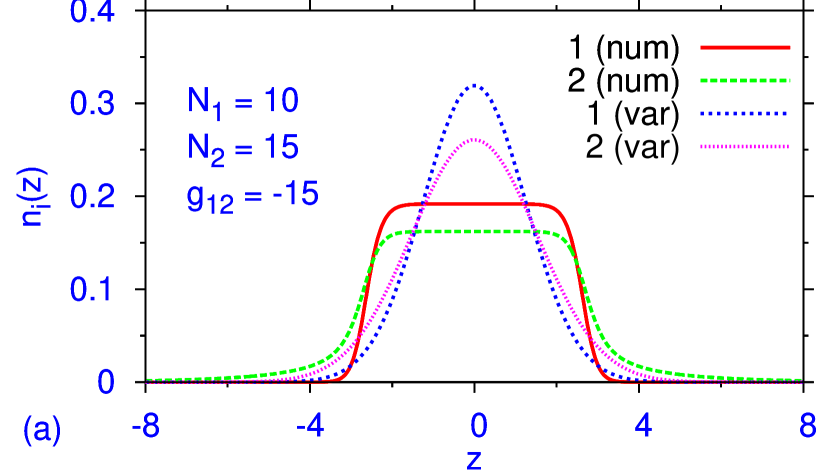
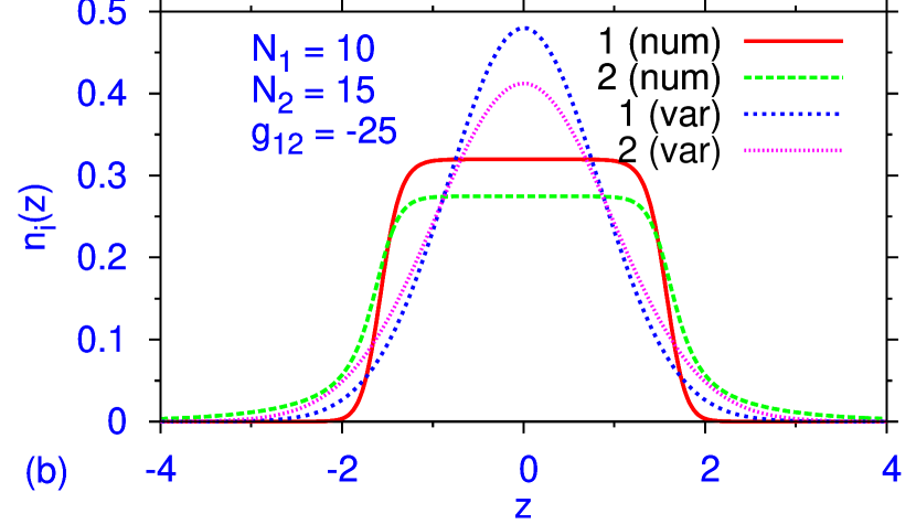
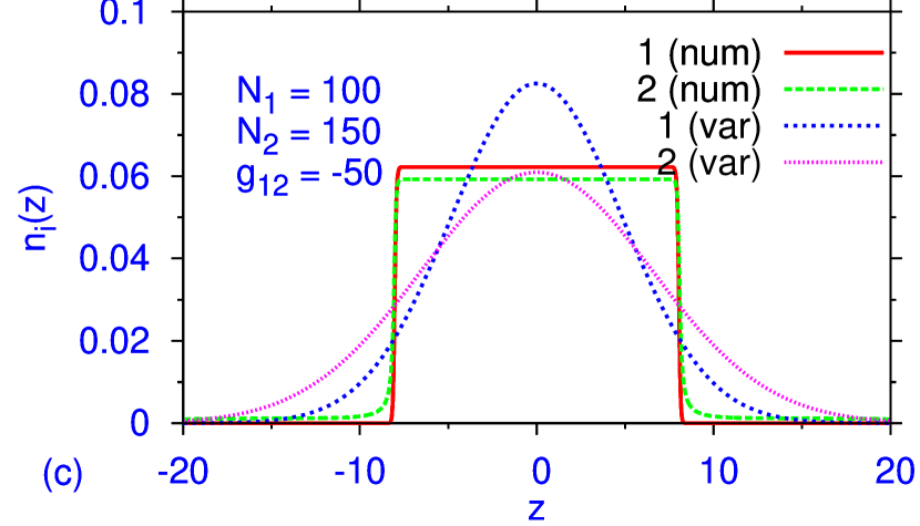
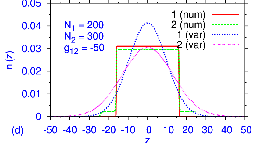
Figure 3: (Color online) Probability densities of the two fermion components from the numerical solution (labelled “num”) of Eqs. (89) and (90) (here normalized to unity: $\int_{-\infty}^{\infty}n_{i}(z)dz=1$) compared with variational results (labelled “var”) given by Eqs. (112) and (113) for $\lambda=1$ and (a) $N_{1}=10,N_{2}=15$ and $g_{12}=-15$, (b) $N_{1}=10,N_{2}=15$ and $g_{12}=-25$, (c) $N_{1}=100,N_{2}=150$ and $g_{12}=-50$, and (d) $N_{1}=200,N_{2}=300$ and $g_{12}=-50$.

IV.4 Numerical Results

For stationary solutions we solve time-independent Eqs. (89) and (90) by using an imaginary time propagation method based on the finite-difference Crank-Nicholson discretization scheme of time-dependent Eqs. (87) and (88). The non-equilibrium dynamics from an initial stationary state is studied by solving the time-dependent Eqs. (87) and (88) with real time propagation by using as initial input the solution obtained by the imaginary time propagation method. The reason for this mixed treatment is that the imaginary time propagation method deals with real variables only and provides very accurate solution of the stationary problem at low computational cost muru . In the finite-difference discretization we use space step of 0.025 and time step of 0.0005.

Figure 4: (Color online) Chemical potential $\mu_{j}$ of $j$th component obtained from the numerical solution (labelled “num”) of Eqs. (89) and (90) and that obtained from the variational results (114) and (115) (labelled “var”) vs. interspecies coupling $g_{12}$ for $N_{1}=200,N_{2}=220$ and $\lambda=1$.

First we report results for stationary profiles of the localized Fermi-Fermi solitons formed in the presence of attractive interspecies interaction (negative $g_{12}$). The fermions form BCS state(s) which satisfy a coupled nonlinear Schrödinger equation with repulsive (self defocusing) quintic nonlinearity. Hence fermions cannot form a bright soliton by itself. However, they can form a bright soliton in the presence of an attractive interspecies interaction skbs induced by varying an external background magnetic field near a Feshbach resonance fesh .

In Fig. 3 we present the soliton profiles of the two components calculated by a direct numerical solution of Eqs. (89) and (90) and compare them with variational results (112) and (113). In general the numerical solutions have a profile distinct from a Gaussian shape of the variational approximation. The numerical density profile reminds of a square barrier. Nevertheless, the variational approximation presents a faithful average description. From Figs. 3 (a) and (b) we find that for a fixed $N_{1}$ and $N_{2}$, as $|g_{12}|$ is increased, the solitons become more compact and are better represented by variational approximation. From Figs. 3 (b) and (c) we see that as the number of fermions is increased the numerical density profiles are more square-barrier type than a Gaussian type. From Figs. 3 (c) and (d) we find that for a fixed $g_{12}$, as the number of atoms is reduced, the solitons become more compact.

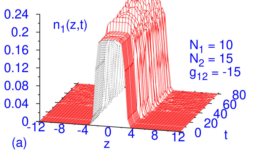
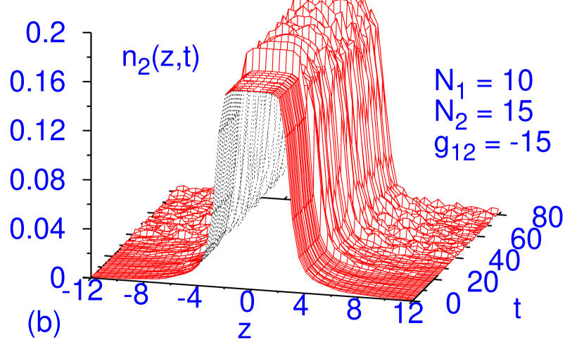
Figure 5: (Color online) Dynamics of the probability density profiles of (a) the first and (b) the second Fermi solitons of Fig 3 (a) when at $t=20$ they are subject to a perturbation by setting $\phi_{j}(z,t)=1.05\times\phi_{j}(z,t).$ The solitons undergo stable propagation as long as we could continue numerical simulation. The initial soliton profile is calculated with imaginary time propagation algorithm and the dynamics studied with real time propagation algorithm. The soliton profiles are normalized to unity: $\int_{-\infty}^{\infty}n_{j}(z,t)dz=1$.

Next we illustrate how well are the variational approximations (114) and (115) for the chemical potential compared to the numerical results. In Fig. 4 we plot the numerically obtained chemical potential for $N_{1}=200,N_{2}=220,$ and $\lambda=1$ for different $g_{12}$ and compare with the variational result. We see that the overall agreement is good for all $g_{12}$, although it is better for small $|g_{12}|$.

After illustrating the soliton profiles in different states it is now pertinent to verify if these solitons are dynamically stable under perturbation. To this end we consider the typical stationary soliton of Fig. 3 (a) (obtained by the imaginary time propagation method) and subject it to the perturbation by setting $\phi_{j}(z,t)=1.05\times\phi_{j}(z,t)$ and observe the resultant dynamics (obtained by the real time propagation method). The resultant dynamics is illustrated in Fig. 5. The solitons under this perturbation execute some oscillation, generate some noise, nevertheless propagate for as long as the numerical simulation was continued without being destroyed. This demonstrates the stability of the solitons under perturbation. For very strong perturbation, as expected, the solitons are destroyed. If time covered by numerical simulation is too short, a unstable solution might appear to be stable. Thus, in numerical simulation it is important to cover times large compared to characteristic timescale of the problem, as in Fig. 5. Also, a false stability might appear for a small interval of time for specific space and time steps used in discretization. We checked the stability for different time steps over large intervals of time.

V Summary

In this paper we have obtained the phase diagram of a BCS superfluid Fermi-Fermi mixture of distinct mass fermions at zero temperature in 1D, 2D, and 3D. The linear stability conditions relating the strength of interspecies Fermi-Fermi interaction with the two Fermi densities are obtained from an energetic consideration. Two possible equilibrium scenarios emerge: a uniform mixture and two pure separated phases. In 1D, two pure and separated phases appear for small fermion densities; for large densities appears the uniform mixture from an energetic consideration as shown in Fig. 1. In 3D, the opposite happens. In addition, in 3D, a mixed and a pure phase can appear. In 2D, the conditions for uniform mixture and separated phases do not put any restriction on the fermion densities but only on the interspecies Fermi-Fermi interaction.

In 3D, the uniform mixture is unstable against small fluctuations for large Fermi densities for a fixed $g_{12}^{2}$. For a positive $g_{12}$ it should show partial demixing and for a negative $g_{12}$ it may undergo collapse. In 1D, the uniform mixture is unstable against small fluctuations for small Fermi densities for a fixed $g_{12}^{2}$. For a positive $g_{12}$ it should show partial demixing and for a negative $g_{12}$ it should form bright solitons. Hence this mixture is of special interest for a negative $g_{12}$. This is the domain of soliton formation by modulational instability of the uniform mixture. To study the modulational instability and soliton formation in the mixture we derive a set of coupled nonlinear equations derived as the Euler-Lagrange equation employing the Lagrangian density of the mixture. The condition of modulational instability so obtained is consistent with that of stability of uniform mixture obtained from an energetic consideration. In addition, we solve the 1D dynamical equations numerically and variationally to study the density and chemical potential of the solitons. The variational result is found to be in good agreement with the numerical solution. We also established numerically the dynamical stability of the Fermi-Fermi solitons by subjecting them to a perturbation by multiplying the wave-function profiles by 1.05. The system is then found to propagate over a very long period of time without being destroyed, which demonstrated the stability of the solitons.

- (1) C. Pethick and H. Smith. Bose-Einstein Condensation in Dilute Gases (Cambridge University Press: Cambridge, 2002); L. P. Pitaevskii and S. Stringari. Bose-Einstein Condensation (Clarendon Press: Oxford and New York, 2003).
- (2) B. DeMarco and D. S. Jin, Science 285, 1703 (1999).
- (3) K. M. O’Hara, S. L. Hemmer, M. E. Gehm, S. R. Granade, and J. E. Thomas, Science 298, 2179 (2002).
- (4) F. Schreck, L. Khaykovich, K. L. Corwin, G. Ferrari, T. Bourdel, J. Cubizolles, and C. Salomon, Phys. Rev. Lett. 87, 080403 (2001).
- (5) A.G. Truscott et al., Sceince 291, 2570 (2001); G. Modugno, G. Roati, F. Riboli, F. Ferlaino, R. J. Brecha, and M. Inguscio, Science 297, 2240 (2002).
- (6) Z. Hadzibabic, C. A. Stan, K. Dieckmann, S. Gupta, M. W. Zwierlein, A. Gorlitz, and W. Ketterle, Phys. Rev. Lett. 88, 160401 (2002).
- (7) C. Ospelkaus, S. Ospelkaus, K. Sengstock, and K. Bongs, Phys. Rev. Lett. 96, 020401 (2006).
- (8) G. Roati, F. Riboli, G. Modugno, and M. Inguscio, Phys. Rev. Lett. 89, 150403 (2002)
- (9) M. W. Zwierlein, J. R. Abo-Shaeer, A. Schirotzek et al., Nature (London) 435, 1047 (2005).
- (10) M. W. Zwierlein, A. Schirotzek, C. H. Schunck et al., Science 311, 492 (2006).
- (11) M. W. Zwierlein, J. R. Abo-Shaeer, A. Schirotzek, C. H. Schunck, and W. Ketterle, Nature (London) 435, 1074 (2005).
- (12) A. L. Fetter and J. D. Walecka, Quantum Theory of Many Particle Systems, (McGraw Hill, New York, 1971).
- (13) In cold atoms Feshbach resonance was first observed in bosonic systems, see, for example, S. Inouye, M. R. Andrews, J. Stenger, H. J. Miesner, D.M. Stamper-Kurn, W. Ketterle, Nature 392, 151 (1998). Later it has been observed in fermionic systems, see, for example, K. M. O’Hara et al., Phys. Rev. A 66, 041401(R) (2002); K. Dieckmann, C. A. Stan, S. Gupta, Z. Hadzibabic, C. H. Schunck, and W. Ketterle, Phys. Rev. Lett. 89, 203201 (2002); T. Loftus, C. A. Regal, C. Ticknor, J. L. Bohn, and D. S. Jin, Phys. Rev. Lett. 88, 173201 (2002); C. A. Regal, M. Greiner, and D. S. Jin, Phys. Rev. Lett. 92, 083201 (2004).
- (14) Feshbach resonance was originally suggested and used in nuclear physics, see, for example, H. Feshbach, Ann. Phys. (NY) 5, 357 (1958); H. Dias, M. S. Hussein, and S. K. Adhikari, Phys. Rev. Lett. 57, 1998 (1986).
- (15) J. R. Schrieffer, Theory of Superconductivity (Benjamin, New York, 1964).
- (16) D. M. Eagles, Phys. Rev. 186, 456 (1969); A. J. Leggett, J. Phys. (Paris) Colloq. 41, C7-19 (1980); P. Nozières and S. Schmitt-Rink, J. Low Temp. Phys. 59, 195 (1985); M. Randeria, Ji-Min Duan and Lih-Yir Shieh, Phys. Rev. B 41, 327 (1990); M. Casas et al, Phys. Rev. B 50, 15945 (1994); S. K. Adhikari et al, Phys. Rev. B 62, 8671 (2000); Physica C 453, 37 (2007).
- (17) M. Greiner, C. A. Regal, and D. S. Jin, Nature (London) 426, 537 (2003); C. A. Regal, M. Greiner, and D. S. Jin, Phys. Rev. Lett. 92, 040403 (2004); J. Kinast, S. L. Hemmer, M. E. Gehm, A. Turlapov, and J. E. Thomas, Phys. Rev. Lett. 92, 150402 (2004).
- (18) M. W. Zwierlein et al., Phys. Rev. Lett. 92, 120403 (2004); M. W. Zwierlein, C.H. Schunck, C. A. Stan, S. M. F. Raupach, and W. Ketterle, Phys. Rev. Lett. 94, 180401 (2005).
- (19) C. Chin et al., Science 305, 1128 (2004); M. Bartenstein et al., Phys. Rev. Lett. 92, 203201 (2004).
- (20) S. K. Adhikari, New J. Phys. 8, 258 (2006).
- (21) K. Mølmer, Phys. Rev. Lett. 80, 1804 (1998); R. Roth, Phys. Rev. A 66, 013614 (2002); P. Capuzzi, A. Minguzzi, and M. P. Tosi, Phys. Rev. A 67, 053605 (2003); M. Modugno et al. Phys. Rev. A 68, 043626 (2003); N. Nygaard and K. Mølmer, Phys. Rev. A 59, 2974 (1999); M. J. Bijlsma, B. A. Heringa and H. T. C. Stoof, Phys. Rev. A 61, 053601 (2000); A. Banerjee, Phys. Rev. A 76, 023611 (2007).
- (22) H. Heiselberg, C. J. Pethick, H. Smith, and L. Viverit, Phys. Rev. Lett. 85, 2418 (2000); L. Viverit, Phys. Rev. A 66, 023605 (2002).
- (23) L. Viverit, C.J. Pethick, and H. Smith, Phys. Rev. A 61, 053605 (2000).
- (24) K.K. Das, Phys. Rev. Lett. 90, 170403 (2003).
- (25) L. Salasnich and F. Toigo, Phys. Rev. A 75, 013623 (2007).
- (26) S.K. Adhikari, Phys. Rev. A 72, 053608 (2005); S.K. Adhikari and B. A. Malomed, Phys. Rev. A 76, xxxxxx (2007).
- (27) G. Modugno et al., Science 297, 2240 (2002); S. K. Adhikari, Phys. Rev. A 70, 043617 (2004).
- (28) K. E. Strecker, G. B. Partridge, A. G. Truscott and R.G. Hulet, Nature 417, 150 (2002); L. Khaykovich, F. Schreck, G. Ferrari, T. Bourdel, J. Cubizolles, L. D. Carr, Y. Castin, and C. Salomon, Science 256, 1290 (2002); V. M. Pérez-García, H. Michinel, and H. Herrero, Phys. Rev. A 57, 3837 (1998).
- (29) S. L. Cornish, S. T. Thompson and C. E. Wieman, Phys. Rev. Lett. 96, 170401 (2006).
- (30) K. E. Strecker, G. B. Partridge, A. G. Truscott, and R. G. Hulet, New J. Phys. 5, 73 (2003); V. A. Brazhnyi and V. V. Konotop, Mod. Phys. Lett. B 18, 627 (2004); F. Kh. Abdullaev, A. Gammal, A. M. Kamchatnov, and L. Tomio, Int. J. Mod. Phys. B 19, 3415 (2005); V. I. Yukalov, Laser Phys. Lett. 1, 435 (2004); A. Minguzzi, S. Succi, F. Toschi, M. P. Tosi, and P. Vignolo, Phys. Rep. 395, 223 (2004).
- (31) T. Karpiuk, K. Brewczyk, S. Ospelkaus-Schwarzer, K. Bongs, M. Gajda, and K. Rzazewski, Phys. Rev. Lett. 93, 100401 (2004); T. Karpiuk, M. Brewczyk, and K. Rzazewski, Phys. Rev. A 73, 053602 (2006).
- (32) S. K. Adhikari, Phys. Lett. A 346, 179 (2005); V. M. Pérez-García and J. B. Beitia, Phys. Rev. A 72, 033620 (2005).
- (33) S. K. Adhikari and L. Salasnich, Phys. Rev. A 75, 053603 (2007)
- (34) S. K. Adhikari, Phys. Rev. A 73, 043619 (2006); S. K. Adhikari and B. A. Malomed, ibid. 74, 053620 (2006).
- (35) S. K. Adhikari, J. Phys. A 40, 2673 (2007); Eur. Phys. J. D 40, 157 (2006); Laser Phys. Lett. 3, 605 (2006); J. Phys. B 38, 3607 (2005); I. Kourakis et al., Eur. Phys. J. B 46, 381 (2005).
- (36) M. Girardeau, J. Math. Phys. 1, 516 (1960); M. Girardeau, Phys. Rev. 139, B500 (1965); L. Tonks, Phys. Rev. 50, 955 (1936); G. E. Astrakharchik, D. Blume, S. Giorgini, L. P. Pitaevskii, Phys. Rev. Lett. 93, 050402 (2004); G. E. Astrakharchik, D. Blume, S. Giorgini, and B. E. Granger, J. Phys. B 37, S205 (2004); P. Öhberg and L. Santos, Phys. Rev. Lett. 89, 240402 (2002).
- (37) T. Kinoshita, T. Wenger, and D. S. Weiss, Science 305, 1125 (2004), B. Paredes et al., Nature 429, 277 (2004).
- (38) K. Huang and C. N. Yang, Phys. Rev. 105, 767 (1957).
- (39) T. D. Lee and C. N. Yang, Phys. Rev. 105, 1119 (1957).
- (40) H. Heiselberg, Phys. Rev. A 63, 043606 (2001).
- (41) N. Manini and L. Salasnich, Phys. Rev. A 71, 033625 (2005)
- (42) J.N. Fuchs, A. Recati, and W. Zwerger, Phys. Rev. Lett. 93, 090408 (2004).
- (43) M. Gaudin, Phys. Lett. 24A, 55 (1967); C.N. Yang, Phys. Rev. Lett. 19, 1312 (1967).
- (44) G. Xianlong, M. Polini, R. Asgari, and M. P. Tosi, Phys. Rev. A 73, 033609 (2006).
- (45) S. Tomonaga, Progr. Theor. Phys. 5, 544 (1950); J.M. Luttinger, J. Math. Phys. 4, 1154 (1963).
- (46) A. Luther and V.J. Emery, Phys. Rev. Lett. 33, 589 (1974).
- (47) V. Ya. Krivnov and A. A. Ovchinnikov, Zh. Eksp. Teor. Fiz. 67, 1568 (1974) [Sov. Phys. JETP 40, 781 (1975)].
- (48) S. K. Adhikari and L. Salasnich, Phys. Rev. A 76, 023612 (2007).
- (49) H. A. Bethe, Z. Physik 71, 205 (1931).
- (50) E. H. Lieb and W. Liniger, Phys. Rev. 130, 1605 (1963); E. H. Lieb, ibid. 130, 1616 (1963).
- (51) I. V. Tokatly, Phys. Rev. Lett. 93, 090405 (2004).
- (52) L. Salasnich, Phys. Rev. A 76, 015601 (2007).
- (53) A. S. Alexandrov and V. V. Kabanov, J. Phys.: Condens. Matter 14, L327 (2002).
- (54) L. Salasnich, S.K. Adhikari, and F. Toigo, Phys. Rev. A 75, 023616 (2007).
- (55) L. Salasnich, Laser Phys. 12, 198 (2002); L. Salasnich, A. Parola, and L. Reatto, Phys. Rev. A 65, 043614 (2002).
- (56) V.V. Konotop and M. Salerno, Phys. Rev. A 65, 021602(R) (2002); L. Salasnich, A. Parola, and L. Reatto, Phys. Rev. Lett. 91, 080405 (2003).
- (57) B. A. Malomed, in Progress in Optics, vol. 43, p. 71 (ed. by E. Wolf: North-Holland, Amsterdam, 2002); V. M. Pérez-García, H. Michinel, J. I. Cirac, M. Lewenstein and P. Zoller, Phys. Rev. A 56, 1424 (1997).
- (58) L. Salasnich, Mod. Phys. Lett. B 11, 1249 (1997); A. Parola, L. Salasnich, and L. Reatto, Phys. Rev. A 57, R3180 (1998).
- (59) S. K. Adhikari and P. Muruganandam, J. Phys. B 35, 2831 (2002); S. K. Adhikari, Phys. Rev. A 69, 063613 (2004); P. Muruganandam and S. K. Adhikari, J. Phys. B 36, 2501 (2003); S. K. Adhikari, Phys. Lett. A 265, 91 (2000); Phys. Rev. E 62, 2937 (2000); W. Z. Bao, D. Jaksch, and P. A. Markowich, J. Comput. Phys 187, 318 (2003).