Regularization of Hele-Shaw flows, multiscaling expansions
and the Painlevé I equation

Abstract

Critical processes of ideal integrable models of Hele-Shaw flows are considered. A regularization method based on multiscaling expansions of solutions of the KdV and Toda hierarchies characterized by string equations is proposed. Examples are exhibited in which the tritronquée solution of the Painlevé-I equation turns out to provide the leading term of the regularization

Key words: Hele-Shaw flows, integrable hierarchies, multiscale expansions, Painlevé-I equation.

1991 MSC: 58B20.

1 Introduction

A Hele-Shaw cell is a narrow gap between two plates filled with two fluids: say oil surrounding one or several bubbles of air. Several dispersionless (quasiclassical) limits of integrable systems have been found [1]-[6] which provide ideal models of Hele-Shaw flows in the absence of surface tension. Moreover, the same integrable structures also arise in random matrix models of two-dimensional quantum gravity [7]. Integrable systems of dispersionless type are solved by means of hodograph equations, so that generic initial conditions reach points of gradient catastrophe in a finite time. In the ideal Hele-Shaw models this feature gives rise to the cusp formation in the motion of the interface, while in random matrix models it manifests itself as the critical points of the asymptotic expansions for large matrix dimension $N$. In both cases a regularization mechanism of the underlying integrable models is required. As it is well known in random matrix theory [7]-[10], the double scaling limit method provides a regularization scheme of the large $N$ expansions which leads to models of two-dimensional quantum gravity. On the other hand, recent work [4]-[6] suggests the use of methods of asymptotic solutions of integrable systems [11]-[13] to cure the singularities in Hele-Shaw flows.

The present work is concerned with the regularization of a family of critical Hele-Shaw processes [4]-[6]. We mainly consider the case in which the interface develops an isolated finger which is close to becoming a cusp [4]-[5]. Then at a small scale the boundary of the finger tip is described by a curve

$$Y(X)=P(X)\,\sqrt{X-v(x,t_{1})},$$

where $(X,Y)$ are Cartesian coordinates, $P(X)$ is a given polynomial and $v(x,t_{1})$ is a particular solution of the dispersionless KdV (Hopf) equation $2\,\partial_{t_{1}}v=3\,v\,v_{x}.$ Here $x\sim Q\,(t-t_{c})$, where $t$ is the physical time, $t_{c}$ is the critical time and $t_{1}$ is a deformation parameter. The starting point of our analysis is the fact that $v$ satisfies the dispersionless limit of the string equations [14] which characterize the one-matrix models of topological and two-dimensional quantum gravity [15]-[17]. Then, from the quasi-triviality property [18] of the KdV hierarchy, there is a unique solution $u$ of the dispersionful KdV equation

$$\partial_{t_{1}}u=\dfrac{1}{4}\,\Big{(}\epsilon^{2}\,u_{xxx}+6\,u\,u_{x}\Big{)},\quad u=\sum_{k\geq 0}\epsilon^{2k}\,u^{(k)},$$ (1)

and its associated hierarchy such that $v=u^{(0)}$. More precisely [14], the $\tau$-function associated with $u$ is the large $N$ limit of the Kontsevich integral over hermitian matrices

$$\tau_{N}(\boldsymbol{t}): =\dfrac{A_{N}(\Theta)}{B_{N}(\Theta)},\quad\Theta:=\mbox{diag}(\theta_{1},\ldots,\theta_{N}),\quad k\,t_{k}=\epsilon\,\mbox{Tr}(-\Theta)^{k},$$

$$A_{N}(\Theta): =\int\mathrm{d}X\,\exp\mbox{Tr}(X^{2}\,\Theta-\dfrac{1}{3}\,X^{3}),\quad B_{N}(\Theta):=\int\mathrm{d}X\,\exp\mbox{Tr}(X^{2}\,\Theta).$$

In this KdV picture, singular Hele-Shaw processes correspond to critical points of the expansion of $u$, which in turn are associated to points of gradient catastrophe for $u^{(0)}$. In our work we follow the same regularization procedure that is used in the one-matrix model description of two-dimensional quantum gravity [8]-[10] : we apply a multiscaling limit method to obtain the leading term of the regularization of $u$ near critical points. Then we use it to continue the Hele-Shaw flow on critical regions. We notice that according to recent work [19, 20], the multiscale regularization of KdV solutions gives a correct asymptotic approximation near the edges of the oscillatory zone (Whitham zone) which emerges at points of gradient catastrophe. We illustrate our strategy by regularizing the $(2,5)$ critical finger studied in [5].

We also consider in this paper the critical processes of break-off and merging of Hele-Shaw bubbles [6]. The same analysis as in the critical finger case applies, but now the ruling integrable structure is supplied by the solution of the Toda hierarchy which underlies the large $N$ limit of the partition function of the Hermitian matrix model

$$\tau_{N}:=\int\mathrm{d}H\exp\Big{(}\mbox{tr}(\sum_{k\geq 1}t_{k}\,H^{k})\Big{)}.$$ (2)

In this case the method is illustrated with an example of regularization for the merging of two bubbles.

Our analysis makes use of the method developed by Takasaki and Takebe [21] for determining solutions of integrable systems by means of string equations (see also [22]-[24]). In the examples considered in both cases, KdV and Toda structures, the leading term of the regularization turns out to be provided by a particular solution of the Painlevé-I equation (P-I)

$$W_{\xi\xi}=6\,W^{2}-\,\xi,$$ (3)

the so called tritronquée solution discovered by P. Boutroux [25]. This is the same function which appears in the study of some critical processes in plasma [26] as well as in the analysis of the critical behavior of solutions to the focusing nonlinear Schrödinger equation [27]. As it is known, a different solution of P-I emerges in the random matrix models of two-dimensional quantum gravity [7].

2 Hele-Shaw flows and the KdV hierarchy

In the set-up considered in [4, 5] the cell is permeable to air but not oil. When air is injected the bubble develops a finger whose tip is pushed away and may become a cusp. By assuming that the finger is symmetric with respect to the $X$-axis and that the cusp is formed at the origin, then near the origin the finger turns to be described by a curve of the form

$$Y(z):=\Big{(}\dfrac{\sum_{k=1}^{l+1}(k+\dfrac{1}{2})\,t_{k}\,z^{2k-1}}{\sqrt{z^{2}-v}}\Big{)}_{\oplus}\,\sqrt{z^{2}-v},\quad X=z^{2}.$$ (4)

Here the subscript $\oplus$ denotes the projection of $z$-series on the positive powers, and $t_{k},\,k\geq 1$ are deformation parameters. The function $v$ stands for the distance between the tip and the origin and it is determined by imposing the asymptotic behaviour

$$Y(z)=\sum_{k=1}^{l+1}(k+\dfrac{1}{2})\,t_{k}\,z^{2k-1}+\dfrac{x}{2\,z}+\mathcal{O}(z^{-3}),\quad z\rightarrow\infty,$$ (5)

where the coefficient $x$ is proportional to time $x\sim Q\,(t-t_{c})$. The resulting equation for $v$ is the hodograph equation

$$H(\boldsymbol{t},v):=\sum_{k\geq 1}(2\,k+1)\,t_{k}\,r_{k}(v)+x=0,$$ (6)

where $\boldsymbol{t}:=(x,t_{1},t_{2},\ldots)$ with $t_{k}=0,\,k>l+1$, and $r_{j}$ are the coefficients of the generating function

$$r:=\dfrac{z}{\sqrt{z^{2}-v}}=\sum_{k\geq 0}\dfrac{r_{k}(v)}{z^{2k}},\quad r_{0}=1.$$

The hodograph equation (6) is the basic piece to solve the system of string equations

$$(z^{2})_{-}=0,\quad(m\,z^{-1})_{-}=0.$$ (7)

for the Lax-Orlov functions of the dispersionless KP (dKP) hierarchy

$$z=p+u_{0}+\mathcal{O}(p^{-1}),\quad m=\sum_{k=1}^{\infty}(2\,k+1)\,t_{k}\,z^{2k}+x+\mathcal{O}(z^{-2}),$$ (8)

$$\{z,m\} :=z_{p}\,m_{x}-z_{x}\,m_{p}=1.$$ (9)

Here and henceforth the subscripts $-$ and $+$ denote the projection of $p$-series on the strictly negative and positive powers, respectively. According to Theorem 1.5.1 of [21], if $(z,m)$ are solutions of (7) satisfying the asymptotic forms (8), then they verify the dKP hierarchy. More concretely, as the first string equation means that $z^{2}=p^{2}+v,$ then the function $v$ verifies the dispersionless KdV (dKdV) hierarchy $\partial_{t_{j}}v=2\,\partial_{x}\,r_{j+1}$.

To solve the second string equation $(m\,z^{-1})_{-}=0$ and satisfy the asymptotic behaviour (8), one sets $m\,z^{-1}=\sum_{k=1}^{\infty}(2\,k+1)\,t_{k}(z^{2k-1})_{+}$. Thus by taking into account that $(z^{2k-1})_{+}=(z^{2k-2}\,r)_{\oplus}\,p$, it follows that (7) reduces to (6). In particular from (4) and (5) we may identify

$$Y(z)=\dfrac{m(z)}{2\,z},$$

so that the dynamics of the curve $Y=Y(X)$ with respect to $\boldsymbol{t}$ is governed by the dispersionless KdV hierarchy. The problem is that near critical points $(\boldsymbol{t}_{c},v_{c})$

$$\dfrac{\partial H}{\partial v}\Big{|}_{\boldsymbol{t}_{c},v_{c}}=\ldots=\dfrac{\partial^{m-1}H}{\partial v^{m-1}}\Big{|}_{\boldsymbol{t}_{c},v_{c}}=0,\quad\dfrac{\partial^{m}H}{\partial v^{m}}\Big{|}_{\boldsymbol{t}_{c},v_{c}}\neq 0,\quad m\geq 2,$$ (10)

the solutions $v$ of (6) are multivalued and have singular derivatives (gradient catastroph). These situations correspond to the critical regimes of the Hele-Shaw fingers described by (4).

In order to find regularizations of these Hele-Shaw flows we consider solutions of the dispersionful version of the KdV equation

$$\partial_{t_{1}}u=\dfrac{1}{4}\,\Big{(}\epsilon^{2}\,u_{xxx}+6\,u\,u_{x}\Big{)}.$$ (11)

and the higher members of its hierarchy $\partial_{t_{j}}\,u=2\partial_{x}R_{j+1}(u)$. Here $R_{j}$ are the Gel’fand-Dikii polynomials determined by

$$\epsilon^{2}\,(R\,R_{xx}-\dfrac{1}{2}\,R_{x}^{\,2})-2\,(z^{2}-v)\,R^{2}+2\,z^{2}=0,\quad R=\sum_{n\geq 0}\dfrac{R_{n}(u)}{z^{2n}},$$ (12)

or by the third-order differential equation

$$\partial_{x}\,R_{n+1}=\Big{(}\dfrac{1}{4}\epsilon^{2}\,\partial_{x}^{3}+v\,\partial_{x}+\dfrac{1}{2}\,u_{x}\Big{)}\,R_{n}.$$ (13)

Our first observation is that there is solvable dispersionful version of the string equations (7) given by

$$(L^{2})_{-}=0,\quad\dfrac{1}{2}(M\,L^{-1}-\dfrac{\epsilon}{2}\,L^{-2})_{-}=0.$$ (14)

Here $L$ and $M$ are Lax-Orlov operators ($[L,M]=\epsilon$)

$$L=\epsilon\,\partial_{x}+u_{1}\,\partial_{x}^{-1}+\cdots,\quad M=\sum_{j\geq 1}(2\,j+1)\,t_{j}\,L^{2\,j}+t_{0}+\mathcal{O}(L^{-2}),$$ (15)

of the dispersionful KP hierarchy. Now, the $\pm$ parts of a pseudo-differential operator denote the truncations of $\partial_{x}$-series in the positive and strictly negative power terms, respectively. According to Proposition 1.7.11 of [21], given a solution $(L,M)$ of (14) satisfying (15) and $[L,M]=\epsilon$, then they are Lax-Orlov operators of the dispersionful KP hierarchy. The first string equation in (14) constitutes the KdV reduction condition and leads to a Lax operator of the form

$$L=(\epsilon^{2}\,\partial_{x}^{2}+u)^{\frac{1}{2}}.$$

The second string equation together with the asymptotic condition on $M$ and $[L,M]=\epsilon$ can be satisfied by setting

$$M\,L^{-1}-\dfrac{\epsilon}{2}\,L^{-2}=\sum_{j=1}^{\infty}(2j+1)\,t_{j}\,(L^{2j-1})_{+}.$$

Thus, by taking into account the identity $[L^{2},(L^{2j+1})_{+}]=-2\epsilon\,\partial_{x}\,R_{j+1},$ the problem reduces to finding solutions of the form

$$u=\sum_{k\geq 0}\epsilon^{2k}\,u^{(k)},$$ (16)

verifying

$$\sum_{k\geq 1}(2k+1)\,t_{k}R_{k}+x=0,$$ (17)

or equivalently

$$\oint_{\gamma}\dfrac{dz}{2\pi i\,z}\,V_{z}\,R\,+x=0,$$ (18)

where $V$ denotes the function $V:=\sum_{j\geq 1}z^{2j+1}\,t_{j}$ and $\gamma$ is a large positively oriented closed path.

To solve this equation for $u$ one may use (12) to determine the coefficients of the $\epsilon$-expansion

$$R=\sum_{n\geq 0}\epsilon^{2n}\,R^{(n)},\quad R^{(0)}\,=\,\frac{z}{(z^{2}-u^{(0)})^{\frac{1}{2}}},$$ (19)

and substitute them in (18) to get the system

$$\oint_{\gamma}\dfrac{dz}{2\pi i\,z}\,V_{z}(z)\,R^{(l)}(z)+\delta_{l0}\,x=0.$$ (20)

From (12), (19) and (20) an iterative scheme for obtaining the expansion (16) of $u$ follows. In particular, for $l=0$ it reduces to the hodograph equation (6) for $u^{(0)}$. This means that the expansion (16) is not valid near critical points (10) so that a different expansion must be used to construct a regularization of the solutions of (6) on critical regions.

3 Multiscaling expansions and asymptotic matching

Given a $m$-th order critical point $(\boldsymbol{t}_{c},v_{c})$ (10) of (6), let us introduce a new small parameter $\tilde{\epsilon}$ and new variables $\tilde{t}_{j}$ and $\tilde{x}$ given by

$$\tilde{\epsilon}:=\epsilon^{\frac{2}{2m+1}},\quad t_{j}=t_{c,j}+\tilde{\epsilon}^{m}\,\tilde{t}_{j},\quad x=x_{c}+\tilde{\epsilon}^{m}\,\tilde{x}.$$ (21)

Let us now look for solutions to (18) of the form

$$u=v_{c}+\sum_{n\geq 1}\tilde{\epsilon}^{n}\,\tilde{u}^{(n)},$$ (22)

where now $R$ is expanded in the form $R=\sum_{n\geq 0}\tilde{\epsilon}^{n}\,\widetilde{R}^{(n)}$. To determine the coefficients of $R$, we first observe that $\epsilon\,\partial_{x}=\tilde{\epsilon}^{1/2}\,\partial_{\tilde{x}}$, so that (12) can be rewritten as

$$\tilde{\epsilon}\,(R\,R_{\tilde{x}\tilde{x}}-\dfrac{1}{2}\,R_{\tilde{x}}^{2})-2\,(z^{2}-u)\,R^{2}+2\,z^{2}=0.$$ (23)

From this equation and taking into account that $v_{c,\tilde{x}}\equiv 0$ one deduces a recursion relation for the coefficients $\widetilde{R}^{(n)}$ and that they can be expressed in the form

$$\widetilde{R}^{(n)}=\widetilde{R}^{(0)}\,\sum_{r=1}^{n}\dfrac{\widetilde{G}_{n,r}}{(z^{2}-v_{c})^{r}},\quad\widetilde{R}^{(0)}\,=\,\frac{z}{(z^{2}-v_{c})^{\frac{1}{2}}},$$ (24)

where the functions $\widetilde{G}_{n,r}$ are differential polynomials in $\tilde{u}^{(k)},\,0\leq k\leq n-r+1$. In particular, from (23) it follows that the leading coefficients $G_{n}:=\widetilde{G}_{n,n},\quad G_{0}=1$ satisfy the same recursion relation as that arising from (12) (with $\epsilon\equiv 1$) for the Gel’fand-Dikii polynomials $R_{n}$. In other words

$$G_{n}=R_{n}(\tilde{u}^{(1)}).$$

If we now substitute (21)-(22) in (18) and identify coefficients of $\tilde{\epsilon}$-powers we get the system of equations

$$\begin{cases}\oint_{\gamma}\dfrac{dz}{2\pi i\,z}\,V_{z}(\boldsymbol{t}_{c})\,\widetilde{R}^{(k)}+\delta_{k0}\,x_{c}=0,\quad k=0,\ldots,m-1,\\ \\ \oint_{\gamma}\dfrac{dz}{2\pi i\,z}\,V_{z}(\boldsymbol{t}_{c})\,\widetilde{R}^{(k)}+\oint_{\gamma}\dfrac{dz}{2\pi i\,z}\,V_{z}(\tilde{\boldsymbol{t}})\,\widetilde{R}^{(k-m)}+\delta_{km}\,\tilde{x}=0,\quad k\geq m.\end{cases}$$ (25)

Since $v_{c}$ is a $m$-th order critical point of (10) we have that

$$\oint_{\gamma}dz\,\dfrac{V_{z}(\boldsymbol{t}_{c})}{(z^{2}-v_{c})^{\frac{2k+1}{2}}}+\delta_{k0}\,x_{c}=0,\quad k=0,\ldots,m-1.$$

Hence, in view of (24) the first $m$ equations of the system are identically satisfied, while the remaining ones determine recursively the coefficients $\tilde{u}^{(n)}$ for $n\geq 1$. In particular for $k=m$ we get the following differential equation for the leading contribution $\tilde{u}^{(1)}$

$$\Big{(}\sum_{j\geq 1}c_{jm}(v_{c})\,t_{c,j}\Big{)}\,R_{m}(\tilde{u}^{(1)})+\sum_{j\geq 1}c_{j0}(v_{c})\,\tilde{t}_{j}+\tilde{x}=0,$$ (26)

where $R_{m}(\tilde{u}^{(1)})$ is the $m$-th Gelfand-Dikii polynomial in $\tilde{u}^{(1)}$ and

$$c_{jr}(v_{c})=(2j+1)\oint_{\gamma}\dfrac{dz}{2\pi i}\,\dfrac{z^{2j}}{(z^{2}-v_{c})^{\frac{2r+1}{2}}}$$

From (26) it follows that $\tilde{v}^{(1)}$ depends on the rescaled variables $\tilde{\boldsymbol{t}}$ through the linear combination $\sum_{j\geq 1}c_{j0}(v_{c})\,\tilde{t}_{j}+\tilde{x},$ so that $\partial_{\tilde{t}_{j}}\,\tilde{u}^{(1)}=c_{j0}(v_{c})\,\tilde{u}^{(1)}_{\tilde{x}}$.

Having in mind the applications to Hele-Shaw flows, we must match the solutions (16) and (22) for $t_{k}=t_{c,k},\,\forall k\geq 1$ and $x$ varying on some overlap interval such us as $\epsilon\rightarrow 0^{+}$ we have $x-x_{c}\rightarrow 0^{-}$ and $\tilde{x}\rightarrow-\infty$. To this end we observe that since ${u}^{(0)}$ satisfies the hodograph equation (6), then near an $m$-th order critical point $(\boldsymbol{t}_{c},v_{c})$ it behaves as

$${u}^{(0)}(x,t_{c,1},t_{c,2},\ldots)\sim v_{c}+\sqrt[m]{c\,(x-x_{c})},\quad c:=-m!\,\Big{(}\dfrac{\partial^{m}H}{\partial u^{m}}(\boldsymbol{t}_{c},v_{c})\Big{)}^{-1}.$$ (27)

Hence, the solutions $u={u}^{(0)}+\mathcal{O}(\epsilon)$ and $u=v_{c}+\tilde{\epsilon}\,\tilde{u}^{(1)}+\mathcal{O}(\tilde{\epsilon}^{2})$ match to first order in $\tilde{\epsilon}$ provided $\tilde{u}^{(1)}$ is a solution of the differential equation (26) such that

$$\tilde{u}^{(1)}\sim\sqrt[m]{c\,\tilde{x}},\quad\tilde{x}\rightarrow-\infty.$$ (28)

Let us illustrate our analysis by studying the (2,5) critical finger considered in [5]. If we set $t_{j}=0$ for all $j\geq 2$ except $t_{3}=2/7$, the hodograph equation (6) for $u={u}^{(0)}$ becomes

$$\dfrac{5}{8}\,u^{3}+\dfrac{3}{2}\,t_{1}\,u+x=0,$$ (29)

so that we have

$${u}^{(0)}\,=\,\left(\frac{2}{5}\right)^{2/3}\left(\sqrt{5(4{t_{1}}^{3}+5x^{2})}-5x\right)^{\frac{1}{3}}-\frac{2\sqrt[3]{\frac{2}{5}}\,{t_{1}}}{\left(\sqrt{5(4{t_{1}}^{3}+5x^{2})}-5x\right)^{\frac{1}{3}}}.$$ (30)

We consider the case $t_{1}<0$ which leads to a cusp of the type $Y^{2}\sim X^{3}$ which can not be continued [5]. The hodograph equation (29) has a $2$-nd order critical point at

$$x_{c}\,=\,-t_{c,1}\sqrt{-\frac{4}{5}t_{c,1}},\quad v_{c}=\sqrt{-\frac{4}{5}t_{c,1}},$$

so that the solution behaves as

$$u\sim v_{c}+\sqrt{-\dfrac{8}{15\,v_{c}}\,(x-x_{c})},\quad x\rightarrow x_{c}^{-}.$$

If we take $t_{1}=t_{1,c}$ (i.e. $\tilde{t}_{1}=0$) equation (26) becomes

$$\tilde{u}_{\tilde{x}\tilde{x}}^{(1)}\,+\,3\,\tilde{u}^{(1)^{2}}\,=\,-\frac{8}{5\,v_{c}}\tilde{x},$$ (31)

and the matching condition requires

$$\tilde{u}^{(1)}\sim\sqrt{-\frac{8}{15\,v_{c}}\tilde{x}}.$$ (32)

By introducing the rescalings

$$W:=-\dfrac{1}{2}\Big{(}\dfrac{5\,v_{c}}{4}\Big{)}^{2/5}\,\tilde{u}^{(1)},\quad\xi:=-\Big{(}\dfrac{4}{5\,v_{c}}\Big{)}^{1/5}\,\tilde{x},$$

we have that the differential equation (31) reduces to the Painlevé I (P-I) equation (3), while the matching condition reads

$$W\sim-\sqrt{\xi/6},\quad\xi\rightarrow\infty.$$ (33)

As it is known [28], the tritronquée solution discovered by P. Boutroux [25] is the unique solution of P-I having no poles in the sector $|\mbox{arg}\,\xi|<4\pi/5$ for sufficiently large $|\xi|$. Moreover, it has no poles on the positive real axis [29].

One may now proceed [27, 29] by taking a numerical approximation to the tritronquée solution for large positive values of $\xi$ and use it to supply initial data for the P-I equation. To this end we have taken the approximation provided by Eq.(3.3) of [28], and have set $t_{1}=t_{c,1}=-\frac{4}{5}$ so that $x_{c}=\frac{16}{25}=0.64$ and $u_{c}=\frac{4}{5}$. Thus, with the aid of the ODE solver of Mathematica we construct a numerical solution that matches with the dispersionless approximation (30). The numerical analysis shows that for $\epsilon=10^{-5}$ we have that $|u^{(0)}-(v_{c}+\tilde{\epsilon}\tilde{u}^{(1)})|<5\cdot 10^{-4}$ in the $x$-interval $(0.6365,0.6395)$. As both functions take values larger than 0.8, the relative error on this interval is smaller than 0.000625. The matching between both solutions on the $x$-intervals $[0.58,0.64022]$ and $[0.6,0.6403]$ can be observed in Fig.1.

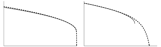
Figure 1: $u^{(0)}$ (solid line) and $u_{c}+\tilde{\epsilon}\tilde{u}^{(1)}$ (dashed line)

In this way, near the critical point the regularized Hele-Shaw dynamics associated to our asymptotic approximation is given by the curve

$$Y(X)\,=\,\left(X^{2}+\frac{u}{2}X+\frac{3}{8}u^{2}-\frac{6}{5}\right)\sqrt{X-u}.$$ (34)

The function $u$ is given by $u^{(0)}(x)$ for $x<0.638$, and by $v_{c}+\tilde{\epsilon}\tilde{u}^{(1)}$ for $x\geq 0.638$. It is defined until a certain $x^{*}$ which corresponds to the first pole of the tritronquée solution on the negative $\xi$-axis. Figures 2 and 3 exhibit a sequence between $x=0.6$ and $x=0.6402302$. Notice that $u$ is a decreasing function of $x$ and that a cusp is formed when one of the roots of the polynomial $P(X)=X^{2}+\frac{u}{2}X+\frac{3}{8}u^{2}-\frac{6}{5}$ coalesces with $u$. Thus, for $x<0.64$ the tip of the finger moves to the left, and it starts forming a cusp as $x$ is close to a certain value slightly higher that $0.64$ ($u$ coincides with the largest root of $P$). Next a bubble appears at the tip of the finger. Subsequently a new cusp forms in this bubble ($u$ coincides with the smallest root of $P$), and a second bubble grows from this cusp while the first bubble declines until it annihilates. Finally, the remaining bubble is absorbed by the finger (when both roots of $P$ coincide).

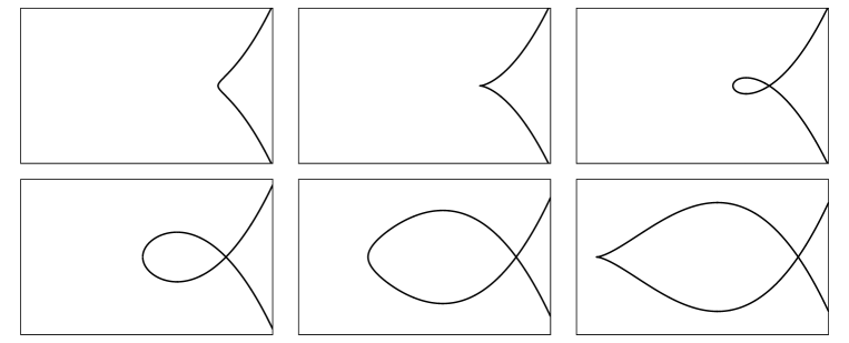
Figure 2: Cusp formation and creation of a bubble which develops a new cusp

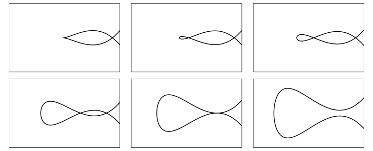
Figure 3: Emergence, annihilation and absorbtion of bubbles

3.1 Hele-Shaw flows and the Toda hierarchy

In the Hele-Shaw set-up considered in [6] air is injected in two fixed points of a simply-connected air bubble making the bubble break into two emergent bubbles. Before the break-off the interface oil-air remains free of cusp-like singularities and develops a smooth neck. The reversed evolution describes the merging of two bubbles.

The analysis of [6] concludes that after the break-off the local structure of a small part of the interface containing the tips of the bubbles falls into universal classes characterized by two even integers $(4\,n,2),\,n\geq 1,$ and a finite number $2n$ of real deformation parameters $t_{k}$. By assuming symmetry of the curve with respect to the $X$-axis, the general solution for the curve and the potential in the $(4\,n,2)$ class are

$$Y(z):=\Big{(}\dfrac{\sum_{k=1}^{2n}(k+1)\,t_{k+1}\,z^{k}}{\sqrt{(z-a)(z-b)}}\Big{)}_{\oplus}\,\sqrt{(z-a)(z-b)},\quad X=z.$$ (35)

where $a$ and $b$ are the positions of the bubbles tips. Due to the physical assumptions of the problem, the expansion

$$Y(z)=\sum_{k=1}^{2n}(k+1)\,t_{k+1}\,z^{k}+\sum_{k=0}^{\infty}\dfrac{Y_{n}}{z^{n}},\quad z\rightarrow\infty,$$ (36)

of the function $Y$ must satisfy two conditions $Y_{0}=t$ (physical time) and $Y_{1}=0$ which determine the positions $a$, $b$ of the tips. As it was shown in [6], imposing these two conditions on (36) leads to a pair of hodograph equations

$$\sum_{k=1}^{\infty}k\,t_{k}r_{k-1}(u,v)=0,\quad\sum_{k=1}^{\infty}k\,t_{k}\,r_{k}(u,v)+2\,x=0,$$ (37)

where $t_{k}=0$ for $k>2n$ and

$$r: =\dfrac{z}{\sqrt{(z-u)^{2}-4v}}=\sum_{k\geq 0}\dfrac{r_{k}(u,v)}{z^{k}},$$

$$a: =u-2\,\sqrt{v},\quad b=u+2\,\sqrt{v}.$$

These equations arise in the dispersionless AKNS hierarcy [6] . However, it is straightforward to see [22] that by setting

$$Y=2\,m-\sum_{k=1}^{2n}(k+1)\,t_{k+1}\,z^{k},\quad x=0,\quad t=t_{1},\quad t_{j}=0,\quad\forall j\geq 2n+2,$$ (39)

they also coincide with the hodograph equations which solve the string equations

$$\bar{z}=z,\quad\overline{m}=m,$$ (40)

for the Lax-Orlov functions

$$z= p+u_{0}+\mathcal{O}(p^{-1}),\quad m=\sum_{k=1}^{\infty}k\,t_{k}z^{k-1}+\dfrac{x}{z}+\mathcal{O}(z^{-2}),$$

$$\bar{z}= \dfrac{v_{0}}{p}+v_{1}+\mathcal{O}(p),\quad\overline{m}=\sum_{=k1}^{\infty}j\,\bar{t}_{k}\bar{z}^{k-1}-\dfrac{x}{\bar{z}}+\mathcal{O}(\bar{z}^{-2}),$$

of the dispersionless 2-Toda (d2-Toda) hierarchy. In particular the first string equation represents the 1-Toda reduction $z=\bar{z}=p+u+v\,p^{-1}$.

In order to regularize the critical points of the hodograph equations (37) one may consider appropriate solutions of the dispersionful version of the Toda hierarchy . The natural candidates are provided by the string equations

$$L=\bar{L},\quad M=\overline{M},$$ (41)

for the Lax-Orlov operators $[L,M]=[\bar{L},\overline{M}]=\epsilon$ of the dispersionful 2-Toda hierarchy [23, 24]. The first equation determines the 1-Toda reduction $L=\bar{L}=\Lambda+u+v\,\Lambda^{-1},\,(\Lambda:=\exp{(\epsilon\,\partial_{x})})$. The system (41) characterizes the partition function of the hermitian matrix model in the large-$N$ limit . In this way the well-known double-scaling limit method for this matrix model can be used to regularize the critical points of (37).

As an example let us analyze the critical process of a merging of two bubbles studied in section VII of [6] . Thus we set $t_{2}=0$, $t_{n}=0$, $n>3$, $t:=t_{1}$ so that (37) reduces to

$$t+3t_{3}\,(u^{2}+2v)\,=\,0,\quad 6t_{3}v\,u+x\,=\,0.$$ (42)

There is a 2nd-order critical point: $v_{c}\,=\,u_{c}^{2},$ with $u_{c}$ satisfying

$$t_{c}+9t_{3}u_{c}^{2}\,=\,0,\quad 6t_{3}u_{c}^{3}+x_{c}\,=\,0,$$ (43)

and consequently

$$4t_{c}^{3}+81t_{3}x_{c}^{2}\,=\,0.$$

On the other hand, the system of string equations (41) of the dispersionful 2-Toda reduces to

$$t+3t_{3}(u^{2}+v+v(x+\epsilon))\,=\,0,\quad 3t_{3}\,(u+u(x-\epsilon))\,v+x\,=\,0.$$ (44)

where $(u,v)$ are characterized by expansions of the form

$$u=\sum_{k\geq 0}\epsilon^{k}\,u^{(k)},\quad v=\sum_{k\geq 0}\epsilon^{2k}\,v^{(2k)}.$$ (45)

Obviously, from (44) it follows that the leading terms $(u^{(0)},v^{(0)})$ satisfy the hodograph equations (37). To deal with solutions of (44) near critical points $(\boldsymbol{t}_{c},u^{(0)},v^{(0)})=(\boldsymbol{t}_{c},u_{c},v_{c})$ of (37), one introduces

$$\tilde{\epsilon}:=\epsilon^{\frac{1}{5}},\quad x\,=\,x_{c}+\tilde{\epsilon}^{4}\tilde{x},\quad t\,=\,t_{c}+\tilde{\epsilon}^{4}\tilde{t}.$$ (46)

It can be proved that (44) admits solutions of the form

$$u\,=\,u_{c}+\sum_{j=2}^{\infty}\tilde{\epsilon}^{j}U^{(j)},\quad v=\,v_{c}+\sum_{j=1}^{\infty}\tilde{\epsilon}^{2j}V^{(2j)}.$$ (47)

Thus, by equating the coefficients of $\tilde{\epsilon}^{j}$ for $j=2,3$ and $4$ in (44) we get

$$U^{(2)}\, =\,-\frac{1}{u_{c}}V^{(2)},\quad U^{(3)}\,=\,-\frac{1}{2u_{c}}V^{(2)}_{\tilde{x}},$$

$$2(V^{(4)} +u_{c}U^{(4)})\,=\,-\frac{\tilde{t}}{3t_{3}}-(U^{(2)})^{2}-\frac{1}{2}\,V^{(2)}_{\tilde{x}\tilde{x}},$$ (48)

$$\frac{1}{2}\partial_{\tilde{x}}^{2} (V^{(2)}-u_{c}U^{(2)})+u_{c}U^{(3)}_{\tilde{x}}-\frac{2}{u_{c}}U^{(2)}V^{(2)}+(U^{(2)})^{2}\,=\,\frac{1}{3t_{3}u_{c}}(\tilde{x}-u_{c}\tilde{t}).$$

This provides us with an expression of $U^{(4)}$ in terms of $(V^{(2)},V^{(4)})$ and implies that $V^{(2)}$ verifies

$$V^{(2)}_{\tilde{x}\tilde{x}}+\frac{6}{u_{c}^{2}}(V^{(2)})^{2}\,=\,\frac{2}{3t_{3}u_{c}}(\tilde{x}-u_{c}\tilde{t}).$$ (49)

Near the critical point the solution of (42) behaves as

$$u\,\sim\,u_{c}\,-\,\frac{1}{3}\sqrt{\frac{1}{t_{3}}(t_{c}-t)},\quad v\,\sim\,v_{c}\,+\,\frac{u_{c}}{3}\sqrt{\frac{1}{t_{3}}(t_{c}-t)}\quad\mbox{as}\quad t\rightarrow t_{c}^{-}$$

so that matching requires a solution of (49) satisfying

$$V^{(2)}\,\sim\,\frac{u_{c}}{3}\sqrt{-\frac{\tilde{t}}{t_{3}}},\quad\mbox{as}\quad\tilde{t}\rightarrow-\infty.$$ (50)

Now, if we set $x=x_{c}=1$ and introduce the change of variables

$$W\,=\,-\left(\frac{2u_{c}^{2}}{3t_{3}}\right)^{-2/5}V^{(2)},\quad\xi\,=-\,\left(\frac{2u_{c}^{2}}{3t_{3}}\right)^{1/5}\tilde{t},$$

it follows that $W$ must satisfy the P-I equation (3) and the asymptotic condition $W\sim-\sqrt{\frac{\xi}{6}}$ as $\xi\rightarrow\infty$, so that it must be the tritronquée solution of P-I.

Thus near the critical point the regularized Hele-Shaw dynamics of this example is characterized by the curve

$$Y(X)=3t_{3}(X+u)\sqrt{(X-u)^{2}-4v},$$

where

$$u=u_{c}-\frac{\tilde{\epsilon}^{2}}{u_{c}}V^{(2)},\quad v=v_{c}+\tilde{\epsilon}^{2}V^{(2)},$$

The resulting process represents the merging of the tips of two bubbles. It turns out that the right bubble develops a cusp, then a new bubble appears at this cusp and it grows until it merges with the tip of the left bubble.

Acknowledgements

The authors wish to thank the Spanish Ministerio de Educación y Ciencia (research project FIS2005-00319) and the European Science Foundation (MISGAM programme) for their support.

References

• [1] M. Mineev-Weinstein, P. Wiegmann and A. Zabrodin, Phys. Rev. Lett. 84, 5106 (2000)
• [2] P. W. Wiegmann and P. B. Zabrodin, Comm. Math. Phys. 213 , 523 (2000)
• [3] I. Krichever, M. Mineev-Weinstein, P. Wiegmann and A. Zabrodin, Physica D 198, 1 (2004)
• [4] R. Teodorescu, P. Wiegmann and A. Zabrodin, Phys. Rev. Lett. 95, 044502 (2005)
• [5] E. Bettelheim, P. Wiegmann, O. Agam and A. Zabrodin, Phys. Rev. Lett. 95, 244504 (2005)
• [6] S-Y. Lee, E. Bettelheim and P. Wiegmann, Physica D 219, 23(2006)
• [7] P. Di Francesco, P. Ginsparg and Z. Zinn-Justin, Phys. Rept. 254,1 (1995)
• [8] E. Brezin and V. Kazakov, Phys. Lett. B 236, 144 (1990)
• [9] M. Douglas and S. Shenker, Nuc. Phys. B 335, 635 (1990)
• [10] D. Gross and A. Migdal, Phys. Rev. Lett. 64, 127 (1990)
• [11] A. V. Gurevich and L. P. Pitaevskii, Sov. Phys. JETP 38(2), 291 (1974)
• [12] P. D. Lax and C. D. Levermore, Comm. Pure a Appl. Math. 36 253, 571, 809 (1983)
• [13] P. Deift, S. Venakides and X. Zhou, IMRN 6, 285 (1997)
• [14] P. van Moerbeke, Integrable Foundations of String Theory, Proceedings of the CIMPA-school, Ed.: O. Babelon, P. Cartier and Y. Kosmann-Schwarzbach, World Scientific, 163 (1994)
• [15] E. Witten, Nuc. Phys. B 340, 281 (1990)
• [16] E. Witten, Surv. in Diff. Geom. 1, 243 (1991)
• [17] M. Kontsevich, Comm. Math. Phys. 147, 1 (1992)
• [18] B. Dubrovin and Y. Zhang, Normal forms of integrable PDEs, Frobenious manifolds and Gromo-Witten invariants arXiv:math/0108160
• [19] T. Grava and C. Klein, Numerical solution of the small dispersion limit of Korteweg de Vries and Whitham equations arXiv:math-ph/0511011
• [20] T. Grava and C. Klein, Numerical study of a multiscale expansion of KdV and Camassa-Holm equation arXiv:math-ph/0702038
• [21] K. Takasaki and T. Takebe, Rev. Math. Phys. 7, 743 (1995)
• [22] L. Martínez Alonso y E. Medina, Phys. Lett. B 641, 466 (2006)
• [23] L. Martínez Alonso and E. Medina, Semiclassical expansions in the Toda hierarchy and the hermitian matrix model, arXiv:0706.0592 [nlin.Si]. To appear in J. Phys. A: Math. Gen.
• [24] L. Martínez Alonso and E. Medina, A common integrable structure in the hermitian matrix model and Hele-Shaw flows, ArXiv:0710.2798 [nlin.Si].
• [25] P. Boutroux, Ann.Ecole Norm, 30, 265 (1913)
• [26] M. Slemrod, European J. Appl. Math. 13, 663 (2002)
• [27] B. Dubrovin, T. Grava and C. Klein, On universality of critical behaviour in the focusing nonlinear Schõdinger equation, elliptic umbilic catastrophe and the tritronquée solution to the Painlevé-I equation arXiv:0704.0501[math.AP]15 May 2007
• [28] A. Kapaev, J. Phys. A: Math. Gen. 37, 11149 (2004)
• [29] N. Joshi and A. Kitaev, Stud. Appl. Math. 107, 253 (2001)