FTUAM 07/13
IFT-UAM/CSIC-07-44
LPT-ORSAY-07-72
arXiv:0710.3672 [hep-ph]
Lepton masses and mixings in orbifold models
with three Higgs families
N. Escudero, C. Muñoz and
A. M. Teixeira
aDepartamento de Física Teórica C-XI, Universidad
Autónoma de Madrid,
Cantoblanco, E-28049 Madrid, Spain
bInstituto de Física Teórica UAM/CSIC, Universidad
Autónoma de Madrid,
Cantoblanco, E-28049 Madrid, Spain
cLaboratoire de Physique Théorique, UMR 8627, Université de
Paris-Sud XI, Bâtiment 201,
F-91405 Orsay Cedex, France
Abstract
We analyse the phenomenological viability of heterotic orbifolds with two Wilson lines, which naturally predict three supersymmetric families of matter and Higgs fields. Given that these models can accommodate realistic scenarios for the quark sector avoiding potentially dangerous flavour-changing neutral currents, we now address the leptonic sector, finding that viable orbifold configurations can in principle be obtained. In particular, it is possible to accomodate present data on charged lepton masses, while avoiding conflict with lepton flavour-violating decays. Concerning the generation of neutrino masses and mixings, we find that orbifolds offer several interesting possibilities.
1 Introduction
At present, string theory is the only candidate to unify all known interactions (strong, electroweak and gravitational) in a consistent way. In addition to necessarily containing the standard model (SM) as its low-energy limit, string theory is expected to address some of its puzzles, namely the nature of masses, mixings and number of families.
From observation, we have firm evidence that Nature contains three families of quarks and leptons, with peculiar mass hierarchies. Moreover, the flavour structure in both quark and lepton sectors is far from trivial, as exhibited by the current bounds on the quark [1] and lepton [2, 3, 4, 5] mixing matrices. At present, we are still lacking two ingredients that are instrumental in understanding flavour dynamics: the discovery of the Higgs boson (which would thus confirm the mechanism of mass generation), and the precise knowledge of how fermions and Higgs scalars interact, that is, the Yukawa couplings of the fundamental theory. In this sense, a theory that aims at successfully explaining the observed fermion spectra, must necessarily be predictive regarding the Yukawa couplings.
Within the context of string theory, a natural and aesthetic solution may arise from orbifold compactifications. In fact, a very interesting way to obtain a four dimensional effective theory is the compactification of the heterotic string [6] on six-dimensional orbifolds [7], and this has proved to be a very successful attempt at finding the superstring standard model [8, 9, 10, 11, 12, 13, 14, 15, 16, 17, 18, 19, 20, 21, 22, 23, 24, 25, 26, 27, 28, 29, 30, 31, 32, 33, 34, 35]. As it was shown in [9, 11], the use of two Wilson lines [7, 8] on the torus defining a symmetric orbifold can give rise to supersymmetric (SUSY) models with gauge group and three families of chiral particles with the correct quantum numbers. These models present very attractive features from a phenomenological point of view. One of the s of the extended gauge group is in general anomalous, and it can induce a Fayet-Iliopoulos (FI) -term [36, 37, 38, 39] that would break SUSY at very high energies (FI scale GeV)). To preserve SUSY, some fields will develop a vacuum expectation value (VEV) to cancel the undesirable -term. The FI mechanism allows to break the gauge group down to , as shown in Refs. [16, 17] and [12].
Orbifold compactifications offer some remarkable properties in relation to the flavour problem. In particular, they provide a geometric mechanism to generate the mass hierarchy for quarks and leptons [40, 41, 42, 43, 44] through renormalisable Yukawa couplings. orbifolds have twisted fields which are attached to the orbifold fixed points. Fields at different fixed points may communicate with each other only by world sheet instantons. The resulting renormalisable Yukawa couplings can be explicitly computed [40, 41, 45, 46, 47, 48, 49, 50, 51] and receive exponential suppression factors that depend on the distance between the fixed points to which the relevant fields are attached. These distances can be varied by giving different VEVs to the -moduli associated with the size and the shape of the orbifold.
Models with purely renormalisable Yukawa couplings, and which are a priori successful from a phenomenological point of view can be obtained if one relaxes the requirement of a minimal SUSY matter content (with just two Higgs doublets) [49]. In fact, orbifolds with two Wilson lines naturally contain three families of everything, including Higgses, and allow for realistic fermion masses and mixings, entirely at the renormalisable level. In this case the low-energy theory corresponds to the minimal supersymmetric standard model (MSSM) with three Higgs families.
Whether or not such values are indeed viable from a phenomenological point of view is a question that deserves careful consideration. Not only should these models correctly reproduce quark and lepton masses and mixings, but they should also comply with the current bounds on flavour-changing neutral currents (FCNCs). Indeed, having three Higgs families, with non-trivial couplings to matter potentially gives rise to FCNCs at the tree-level [52, 53, 54, 55]. In previous studies [56], we have addressed the phenomenology of the Higgs and quark sectors of models with two Wilson lines. We have verified that quark masses and mixings could be reproduced, and that FCNCs in the neutral -, - and -sectors could be avoided by a fairly light Higgs spectrum. It is worth recalling that, after fitting the quark data, the free parameters defining the orbifold geometry are already very constrained.
In this work, we complete our previous analyses, by investigating whether or not the orbifolds can also succeed in accommodating present data on charged lepton masses, while avoiding conflict with lepton flavour violating (LFV) tree-level processes, such as three-body decays. Finally, and most interesting, is the question of complying with experimental data on neutrino mass squared differences and mixing angles. This analysis is particularly challenging since, as we will discuss, orbifolds offer a variety of possibilities to account for the smallness of neutrino masses.
Let us recall that the experimental observation of neutrino oscillations has led to extend the SM in order to accommodate non-vanishing neutrino masses. In the absence of a predictive theory for the Yukawa couplings, it is only common to argue that purely Dirac neutrinos pose a naturalness problem, in the sense that the associated couplings are extremely tiny. Moreover, and contrary to what is observed in the quark sector, the leptonic mixing, parameterised by the Maki-Nagakawa-Sakata matrix, [57, 58],is nearly maximal. orbifolds offer several possibilities for the generation of neutrino masses and mixings, ranging from a purely Dirac formulation, to several implementations of a type-I seesaw mechanism [59]. Here we will argue on the viability of each possibility.
This paper is organised as follows. In Section 2 we conduct a brief overview of the main properties of Yukawa couplings in this class of orbifold compactifications. In Section 3, we summarise the most relevant features of the extended Higgs sector. The additional constraints on the orbifold parameters obtained from reproducing the charged lepton masses are presented in Section 4, where we also discuss the tree-level contributions to LFV processes. In Section 5, we comment on the implications of the phenomenologically derived constraints regarding the properties of the compact space. Section 6 is devoted to the discussion of the viability of several mechanisms regarding the generation of neutrino masses and mixings. We summarise our findings in Section 7.
2 Yukawa couplings in orbifold models
In this Section we briefly review the most relevant features of the geometrical construction of the orbifold leading to the computation of the fermion mass matrices.
The construction is made by dividing the space by a root lattice modded by the point group (P) with generator , where the action of on the lattice basis is , , with . The two-dimensional sublattices associated to are presented in Figure 1.

In orbifold compactifications, twisted strings appear attached to fixed points under the point group. In the case of the orbifold there are 27 fixed points under P, and therefore 27 twisted sectors. We will denote the three fixed points of each two-dimensional lattice as (). The general form of the Yukawa couplings between the twisted fields in orbifolds is given by the Jacobi theta function (see, for example, the Appendix of Ref. [48]). These Yukawa couplings contain suppression factors that depend on the relative positions of the fixed points to which the fields involved in the coupling are attached, and on the size and shape of the orbifold (i.e. the deformation parameters). Imposing invariance under the point group reduces these parameters to nine: the three radii of the sublattices and the six angles between complex planes. The latter parameters correspond to the VEVs of nine singlet fields appearing in the spectrum of the untwisted sector, and which have perturbatively flat potentials. These so-called moduli fields are usually denoted by . In the most simple assumption, i.e. when the six angles are zero, there are only three relevant parameters which characterise the whole compact space.
Assuming that the two non-vanishing Wilson lines correspond to the first and second sublattices, then the 27 twisted sectors come in nine sets with three equivalent sectors in each one. The three generations of matter (including Higgses) correspond to changing the third sublattice component () of the fixed point, while keeping the other two fixed. Consider for example the following assignments of observable matter to fixed point components in the first two sublattices,
| (1) |
In this case, the fermion mass matrices before taking into account the effect of the FI breaking, are given by the following expression [49]:
| (2) |
where
| (3) |
is the gauge coupling constant, and is related to the volume of the lattice unit cell such that . In the above matrices denote the VEVs of the neutral components of the six Higgs doublet fields. Since we are assuming an orthogonal lattice, i.e. with the six angles equal to zero, only the diagonal moduli (which are related to the radii of the three sublattices) contribute to the Yukawa couplings, through the suppression factors
| (4) |
The existence of an anomalous in the extended gauge group generates a Fayet-Iliopoulos -term which could in principle break SUSY at energies close to the string scale. This term can be cancelled when scalar fields (), which are singlets under , develop large VEVs ( GeV). The VEVs of these fields (), have several important effects. Firstly, they break the original gauge group down to the (MS)SM . Secondly, they induce very large effective mass terms for many particles (vector-like triplets and doublets, as well as singlets), which thus decouple from the low-energy theory. Even so, the SM-like matter remains massless, surviving as the zero mass mode of combinations with the other (massive) states. All these effects modify the mass matrices of the low-energy effective theory (see Eq. (2)), which, for the example studied in [49], are now given by
| (5) |
where are the Higgs VEV matrices prior to FI breaking (see Eq. (3)), is given by
| (6) |
with , and is the diagonal matrix defined as
| (7) |
Finally
| (8) |
In the above, are derived from the VEVs of the heavy fields responsible for the FI breaking as
| (9) |
where in each case and can take any of the following values:
| (10) |
Let us also stress that one should not take , , and as independent parameters. In fact, Eqs. (6,8) imply that
| (11) |
so that for given values of and , is fixed as
| (12) |
The most striking effect of the FI breaking is that it enables the reconciliation of the Yukawa couplings predicted by this scenario with experiment. In particular, as it has been shown [56], the quark spectrum and a successful Cabibbo-Kobayashi-Maskawa (CKM) matrix can now be accommodated. Moreover, expanding the eigenvalues of the quark mass matrices up to leading order in , one can derive the following relation for the Higgs VEVs in terms of the quark masses
| (13) |
3 The extended Higgs sector
As it has been previously discussed, this class of orbifold models contain naturally a replication of Higgs families. In this section we will summarise those features of the Higgs sector relevant for the present analysis (for a more complete study of generic SUSY models with three Higgs generations, see Ref. [55]).
By construction, let us consider an orbifold scenario containing three generations of Higgs doublet superfields, with hypercharge and , respectively coupling to down- and up- type quarks.
| (14) |
We assume the most general form of the superpotential for the quarks and leptons, which is given by
| (15) |
where and denote the quark and lepton doublet superfields, and are quark singlets, and , , the lepton singlet superfields. The Yukawa matrices can be deduced from Eq. (2). In what follows, we take the as effective parameters.
The scalar potential receives the usual contributions from -, - and SUSY soft-breaking terms, which we write below, using for simplicity doublet components.
| (16) |
After electroweak (EW) symmetry breaking, the neutral components of the six Higgs doublets develop VEVs, which we assume to be real,
| (17) |
For the purpose of minimising the Higgs potential and computing the tree-level Higgs mass matrices, it proves more convenient to work in the so-called “Higgs basis” [52, 60], where only two of the rotated fields develop VEVs:
| (18) | |||
| (19) |
By construction, in order to comply with EW symmetry breaking, the new VEVs must satisfy
| (20) |
and we can now introduce a generalised definition for :
| (21) |
In the new basis, the free parameters at the EW scale are , , which has dimensions mass2, and (for a detailed discussion of the Higgs basis, including the definition of the new parameters and of , we again refer the reader to [55]), and the minimisation equations simply read:
| (22) |
The Higgs spectrum derived from the tree-level potential and the previous conditions is far richer than in the usual MSSM case. The neutral sector consists of six CP-even and five CP-odd scalars, while the charged sector will contain ten mass eigenstates. This provides not only a more challenging scenario for potential Higgs detection, but also allows the appearance of dangerous tree-level FCNCs which are severly constrained by observation. The phenomenology related to this multiple-Higgs model and the effects on quark flavour changing transitions have been previously studied in [56]. The impact on lepton flavour violating processes will be discussed in Section 4.2.
4 Charged leptons
As mentioned in the Introduction, the previous analysis [56] of the orbifold parameter space has already severely constrained the free parameters of the orbifold. As discussed, we have verified that one could successfully reproduce the observed hierarchy and mixings in the quark sector, and avoid potentially dangerous tree-level FCNCs with a fairly light Higgs boson spectrum. In what follows, we extend our analysis to the lepton sector. In this section we address how reproducing the charged lepton masses further constrains the orbifold parameters, and also discuss possible tree-level lepton flavour violation, arising from the exchange of neutral Higgses.
4.1 Charged lepton masses
We start by considering the mass matrix for the charged leptons, which after FI breaking is given by111Note that the expression for the matrix in Eq. (26) corrects the misprint in Ref. [49], Eq. (69), where the matrix product was taken in the order . A similar correction for neutrino masses will be subsequently taken into account in Eqs. (47) and (57).
| (26) |
where , and have been defined in Eqs. (3, 6-8), setting . The next step in the analysis is to determine whether one can find regions of the parameter space where the charged lepton masses can be obtained. We recall that most of the variables appearing in Eq. (26), namely , , and the Higgs VEVs are also related to the quark sector of the model, and are thus already tightly constrained [56]. We consider the quark input sets studied in Ref. [56], used to fix the six Higgs VEVs, and which correctly reproduce the correct mass spectrum for both the up- and down-quarks :
| (27) | |||
| (28) | |||
| (29) | |||
| (30) |
and scan over the , and intervals compatible with realistic quark masses and mixings,
| (31) |
The value of , which is also crucial, is tightly related to [56]. From the previous values, and employing Eqs. (2), (20) and (21), we can also derive the value of , which is obtained from the following expression:
| (32) |
Thus, once the several orbifold parameters are determined, one can derive information on the intrinsic orbifold properties, such as the value of the orbifold normalisation constant , or the heterotic coupling constant . The numerical analysis of this subsection is instrumental in obtaining the latter information.
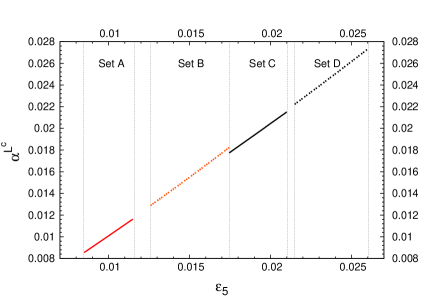
Having set the quark parameters and choosing as an example, we proceed to determine , , and . These values will in turn allow to derive the mass matrix for the charged leptons. In agreement with experimental data [1], the latter eigenvalues should be
| (33) |
 |
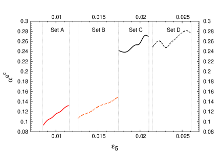 |
we present the values of and giving rise to the correct masses for both the quark and the charged-lepton sectors. The scan over has been conducted for the four quark sets in Eqs. (27 -30). We can see that the behaviour of is completely analogous to what had been observed for the quark sector [56], which is not unexpected, given that the Yukawa couplings for the charged leptons closely follow those of the down-type quarks.
Let us comment on the suppression factor . As seen from Eq. (26), is a global factor in the charged-lepton mass matrix. This allows its value to be modified without affecting the mass eigenstates, provided that (i.e. the ratio of the Higgs VEVs) is accordingly changed. In other words, is still an unconstrained degree of freedom, a fact that is particularly useful for the analysis involving the Higgs sector (as discussed in [55]).
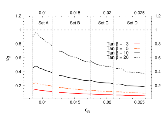
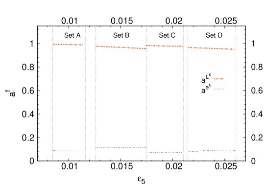
In Figure 4 we display the relation between and for four different values of . It is worth mentioning here that, given a particular quark input set, the value of is bounded from above in order to avoid . For example, for set A this bound is close to . In fact, and as already noticed in the study of the quark sector, the phenomenological viability of these orbifold constructions favours lower values of (not only based on reproducing a viable spectrum, but also related with avoiding excessive FCNCs).
Not only can the quantities be understood as suppression factors which affect the Yukawa couplings (providing the desired mass hierarchy between fermions), but they are also subject to perturbativity constraints. Concerning the latter, for example is actually given by [49]
| (34) |
where the last approximation corresponds to the assumption of Eq. (4). Clearly, if are in general large, have to be small, and therefore perturbativity is spoiled. Under the approximation of Eq. (4), one can write
| (35) |
and, as a consequence, we verify that cannot be larger than 3, since the VEVs are proportional to , and therefore positive. From the analysis of the orbifold parameters, one can obtain useful information about the high-energy configuration of the string model, namely the size and properties of the compact space, as well as its relation with the gauge unification scale. The allowed regimes for the three and their physical implications will be studied in detail in Section 5.
4.2 Tree-level lepton flavour violation
Identical to what occurs for the quark sector, having a model with Higgs family replication opens the possibility of tree-level FCNCs in the lepton sector, contrary to what occurs in the SM or in the MSSM. Given the fact that flavour-violating interactions are very suppressed in Nature, one should ensure that the present model does not induce excessively large contributions to these processes. In a general multi-Higgs model, it is widely recognised that the most stringent bounds arise from the smallness of the masses of the long- and short-lived neutral kaons. It has been previously verified [56] that for a relatively light Higgs boson spectrum of order TeV, the present orbifold model is in very good agreement with experimental data. The analysis was also extended to the - and -meson systems, leading to similar bounds for the Higgs masses. With the inclusion of the charged lepton sector in our analysis, it is only natural to expect dangerous lepton flavour-violating interactions. Regarding these interactions, here we have focused on the branching ratios (BRs) of pure leptonic decays of the type , which have been identified in the literature as the less suppressed processes [53, 54]. In the context of the present orbifold model, these decays are going to be generated by Yukawa interactions mediated by neutral Higgs bosons222We stress here that there are no tree-level contributions to other LFV processes, like radiative decays of the type , which only occur at one-loop level.. As shown in recent studies of LFV in SUSY models with one Higgs family [61, 62, 63], the one-loop contributions to flavour violating processes can be extremely large for sizable values of and a Higgs mass of order 100 -150 GeV. In our case, and as will be shortly confirmed, the requirement that the Higgs bosons are heavy enough to suppress the dangerous quark FCNC interactions indeed ensures that the leptonic processes remain several orders of magnitude below the respective experimental bounds.
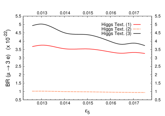
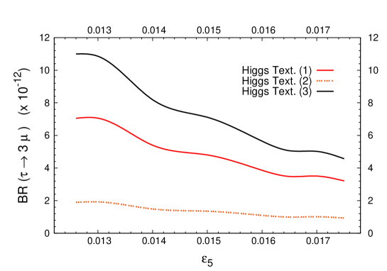
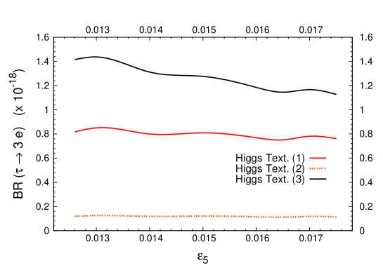
In order to study the occurrence of tree-level LFV in the charged-lepton sector we consider the branching ratios of three-body decays, , mediated by a neutral physical Higgs eigenstate (). The transition amplitudes and BRs of these processes are then given by
| (36) |
where is the lepton mass, the mass of the mediating scalar/pseudoscalar neutral Higgs, and is the element of the Yukawa coupling matrix, in the physical mass-eigenstate basis, defined as
| (37) |
In the above, the Higgs physical states are related to the original interaction eigenstates by , where are the neutral components of the Higgs doublets (see Eq. (14)). and are the matrices which diagonalise the charged-lepton mass matrix, and (with ) are the three charged-lepton Yukawa matrices associated to the down-type Higgses, as shown in Eq. (3). Using the above expressions, we can now compute the contributions of the full Higgs spectrum (six scalars and five pseudoscalars) to the LFV decays. To do so, we choose three distinct Higgs mass textures, already considered in a previous study [56]. Working in the Higgs basis (see Section 3) these can be summarily defined via the following parametrisation, which allows to define the Higgs sector via six dimensionless parameters as
| (38) |
In the above, should be understood as the () submatrices of the matrix that encodes the rotated soft-breaking Higgs masses in the Higgs basis (see [55]). The symbol denotes an entry which is fixed by the minima conditions of Eq. (22). For the Yukawa matrices, we will employ the quark Set A of Eq. (27) and those values of , and compatible with realistic masses for the charged leptons (as analysed in Section 4). Other sets for the quark masses, B, C or D, will lead to similar results. For simplicity, we will take a near-universality limit for the Higgs-sector textures introduced in Eq. (38). Regarding the value of , and unless otherwise stated, we shall take in the subsequent analysis. We consider the following three cases, with the associated tree-level scalar and pseudoscalar Higgs spectra:
-
(1)
GeV ;
GeV .
-
(2)
GeV ;
GeV .
-
(3)
GeV ;
GeV .
In the above, and respectively denote the values for the physical scalar and pseudoscalar masses. The results for the decays , and are summarised in Figs. 5, 6 and 7. From the latter, we immediately observe that the Higgs-mediated contributions to the branching ratios always lie several orders of magnitude below the experimental limits (collected in Table 1). This occurs even for Texture (1), associated with a spectrum containing only light (below 1 TeV) Higgs particles.
Regarding other relevant LFV processes, as for example leptonic conversion processes in heavy nuclei, which could in principle also receive important tree-level contributions, we have not discussed them here, as these conversion processes are always assumed to be of the same order or even sub-dominant with respect to the leptonic decays (see, for example, [53], [54] or [67]). The extremely low contribution to the purely leptonic decays previously studied (between 5-10 orders of magnitude below the present experimental bounds) renders the impact of these LFV processes clearly negligible, when compared to the flavour-changing processes occurring in the quark sector.
5 Orbifold analysis at the string scale
With the full determination of the quark and charged-lepton sectors we are now ready to address the implications of imposing phenomenological viability at the string level. As previously discussed, the characterisation of the orbifold model is tightly related to the determination of the geometrical suppression factors, , which in turn are instrumental in complying with the different fermion mass hierarchies. As we will discuss in Section 6, will further affect the neutrino Yukawa couplings, with an important impact on the seesaw scale. At this point, it is also relevant to mention that we will not take into account the effect of the renormalisation group equations (RGE) on the quark and lepton mass matrices presented in the previous sections. The flavour structure for the masses is associated with a mechanism taking place at a very high energy scale. However, and given the clearly hierarchical structure of the mass matrices, one does not expect that RGE running will significantly affect the predictions of the model.
In this section, we briefly comment on the information about the shape and size of the compact space, and also discuss the hints on the gauge properties of the string model, which can be inferred from the already constrained values of .
Let us firstly consider the value of the product of the heterotic coupling constant, , by the orbifold normalisation constant , defined in Eq. (32). The normalisation constant is given by
| (39) |
In the latter, denotes the volume of the unit cell of the lattice,
| (40) |
where are the unit cell radii in each sublattice, defined in terms of the three -moduli as
| (41) |
From Eq. (32), taking only the dominant terms into account, we can verify that the assumption of [49] is indeed valid for values of , and , since
| (42) |
 |
 |
 |
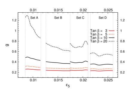 |
where we have used the relation between the orbifold parameters given by Eq. (11). In Fig. 8 we display (as presented in Ref. [56]) the diagonal moduli and for different values of . In Figure 9 we show the correlation between those values of the moduli compatible with correct charged-lepton masses and , for different values of . From all plots we are led to verify that , implying that the sizes of the radii in each orbifold sublattice are comparable and of order
| (43) |
As it was previously shown in Section 4.1, Eq. (35), the upper bound for the suppression factors is 3, above which the moduli are no longer a positive quantity. In the case of and , the values are always fixed by the choice of a given , as we can see in the previous plots. This in turn implies the existence of an upper limit for , above which the moduli become zero. In general, this occurs for values of between 30 and 40, depending on the choice of the remaining orbifold parameters.
In the first analysis of Ref. [56], the constraints on the orbifold parameters derived from the quark sector had already allow to hint towards a range for the product , . The inclusion of the bounds arising from considering the lepton sector finally allows to refine the knowledge of these orbifold parameters. On the left hand-side of Fig. 10 we show the value of the orbifold normalisation constant for different values of as a function of . From this plot, using Eq. (42), we can derive the value of the heterotic gauge coupling constant . The result is presented on the right hand-side of Fig. 10. As we observe, for the chosen regimes of , the value of varies between . It is worth noticing here that a value of of order 1, which is compatible with the above result, was obtained in the orbifold models with three Higgs families analysed in [26], in order to solve the discrepancy between the unification scale predicted by the heterotic superstring ( GeV) and the value deduced from LEP experiments ( GeV).
6 Neutrinos
As seen from the previous sections, after having imposed the requirements of viable quark masses and mixings, as well as the correct charged lepton masses, many of the orbifold parameters have already been constrained. The question that remains to be answered is whether or not the present neutrino data can be reproduced. In the following subsections, we will discuss how the orbifold model allows us to deal with the problem of neutrino masses, providing several mechanisms that can potentially account for an experimentally viable mass spectrum and MNS matrix, including in some of the cases the generation of an effective seesaw mechanism.
6.1 Dirac neutrino masses without seesaw
In the present orbifold model, the simplest way of obtaining massive neutrinos is to assume that the latter are Dirac particles, and introduce a Yukawa term, coupling left- and right-handed neutrinos to the up-type Higgs fields. Accordingly, the Dirac mass matrix for the neutral leptons is given by:
| (47) |
where , and are defined in Eqs. (3) and (6 - 8). As shown in [49], unless some fine-tuning is introduced in the model the use of these terms without the addition of Majorana couplings gives rise to excessively heavy neutrinos. This can be easily understood by noticing that all the parameters involved in Eq. (47) are completely determined from the quark and charged-lepton sectors, the only exception being (and thus and ). Thus, the mass eigenvalues of the Dirac neutrinos can be approximately written as:
| (48) |
leading to the relation
| (49) |
Regarding the three parameters appearing in the previous equation, is defined by the chosen value of (see [56]). For between 3 and 20, values of compatible with realistic quark masses lie in the range . The factor has been determined from the charged-lepton sector, . Thus the remaining free parameter in Eq. (49) is , which depends on and in the following way (see Eq. (11)):
| (50) |
Suppression of the light neutrino masses requires values of very close to 1, forcing to be very small. In turn, this would imply that there are additional fields entering the FI breaking, with a very distinct mass hierarchy (much lighter VEVs), giving rise to terms of the form
| (51) |
To clarify the latter statement, and as an example, let us consider the case in which the factors and , defined in Eq. (9), are taken to be and . In this case, Eq. (51) may be rewritten as
| (52) |
In order to fulfil the above condition, we are compelled to modify the original hypothesis of assuming the VEVs to be of the order of the FI breaking scale, i.e. GeV. One possibility of obtaining the desired hierarchy between and is to invoke the existence of effective non-renormalisable couplings of the form
| (53) |
where denote two extra-matter fields which should later mix with the field [49]. Although this possibility may solve the discrepancy between the FI-breaking scale and the one needed to comply with realistic neutrinos, the introduction of non-renormalisable couplings sets an undesired arbitrariness in the mass scales used to generate the fermion masses. In this sense, it seems preferable to find another way to generate neutrino masses without the addition of higher-order operators.
Another possible solution to this problem could lie in the assumption of a more involved mixing of the fields participating in the FI breaking, as will be presented in Section 6.3. Nevertheless, a more straightforward and simple possibility consists of assuming that the neutrinos are Majorana particles. In this case, one allows the presence of Majorana terms in the superpotential, leading to a type-I seesaw mechanism. There are several possible ways of implementing a seesaw mechanism in the context of these orbifold models, and we pursue this topic in the following subsections.
6.2 Neutrino masses via a type-I seesaw
As first proposed in [49], the introduction of a seesaw mechanism can be easily achieved by considering a Majorana term in the superpotential, arising from the coupling of three extra scalars (of the low-energy spectrum) as follows:
| (54) |
where are singlets assigned to the following fixed-point components in the first two sublattices:
| (55) |
Under this assumption, when the singlets develop a VEV, a Majorana mass for the right-handed neutrinos is generated. In the seesaw limit, where the latter VEVs are much heavier than the EW scale, the effective mass matrix for the light neutrinos is then
| (56) |
where is given in Eq. (47) and arises from the coupling , and is thus defined as
| (57) |
with
| (61) |
being the singlet VEVs. Note that in Eq. (56) the mixing cancels, so that the only free parameters in the mass matrix will be the VEVs . It is also important to stress at this point that the Majorana mass term in Eq. (56) is clearly non-diagonal, with a structure which is determined from the orbifold (analogous to what occurs for all the Dirac mass terms).
The study of the parameter space generated by (for different regimes of the other parameters) reveals that it is possible to generate light neutrino masses of the desired order of magnitude, in good agreement with the experimentally measured mass squared differences between the three species, and (see, for example, [2]),
| (62) | |||||
| (63) |
To illustrate this mechanism, let us define the seesaw mass matrix as it would arise from the following point in the orbifold parameter space, compatible with realistic quark (Set B, Eq. (28)) and charged-lepton masses,
| (64) |
Setting , the only remaining parameters in the model are the singlet VEVs . The choice of the following values
| (65) |
gives us a “normal hierarchy” light neutrino spectrum,
| (66) |
leading to mass squared differences in good agreement with the experimental range of Eqs. (62, 63). Even though this implementation of a type-I seesaw mechanism can lead to a viable light neutrino spectrum, there are two drawbacks to this formulation. The first one comes from the high scale required by the Majorana singlets ( GeV). Again, a possible explanation of this high scale is to assume the fields as effective non-renormalisable FI fields (analogous to the ones suggested in Eq. (53)) or to allow a more complicated FI mixing which would translate into a further suppression of the Yukawa couplings (see Section 6.3, below). The second shortcoming stems from a failure in reproducing the observed mixing in the leptonic sector, as parameterised by the the matrix
| (70) |
where, for simplicity, we use the CP-conserving parametrisation. The mixing angles , , , are experimentally333We employ the values given in [2]. given by
| (71) | |||||
| (72) | |||||
| (73) |
where the angles are expressed in degrees. With the choice of orbifold parameters used in the previous example, Eq. (64), we find that in this case the mixing angles in the matrix are
| (74) |
As can be verified, the above values lie considerably above the ones allowed by the experimental bounds. The associated would then be given by
| (78) |
This matrix contains nearly the desired mixing for the second and third generations, but fails in reproducing the mixing for the first generation of neutrinos. This behaviour is generic to the surveyed orbifold parameter space, where we have systematically found that no more than two-generation mixing can be satisfied. By varying the singlet VEVs other mixing possibilities can be achieved, but one generation of neutrinos never has a viable mixing with the other two. This appears to be a general feature of the present orbifold model, in the sense that it is extremely difficult to simultaneously accommodate the observed near-maximal mixing in the lepton sector and the small one evidenced in the CKM matrix.
A second possibility of implementing a type-I seesaw, without the need of considering a more intricate FI breaking, consists in assuming the existence of an intermediate scale. In principle this scale is not predicted by the orbifold formulation, but it would nevertheless allow to accommodate the experimental data in view of orbifold-derived neutrino Yukawa couplings. In particular, in this case one is allowing for additional sources of unconstrained mixing in the lepton sector, stemming from heavy Majorana neutrino interactions. Thus the effective light neutrino mass matrix is obtained from the seesaw equation, and given by
| (79) | ||||
| (80) |
where is defined in Eq. (47) and is the Majorana mass matrix, whose values are not determined by orbifold considerations. In general, , are known and a very simple structure is adopted for (namely a diagonal matrix) in order to derive the unknown Yukawa couplings. In the present approach, we do know the Yukawa couplings (from the orbifold construction, which at this stage has become strongly constrained), and phenomenological viability of the orbifold scenario indirectly suggests the structure of . Noticing that the seesaw equation can be rewritten as
| (81) |
we obtain as required to comply with data on neutrino masses and mixings. It is important to notice that we are not working in a basis where the charged lepton Yukawa couplings are diagonal, implying that the matrix is defined as
| (82) |
where is the unitary matrix that rotates the left-handed charged lepton fields, so to diagonalise , while is the matrix that diagonalises the symmetric neutrino mass matrix, .
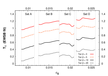
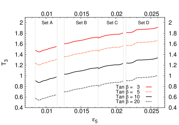
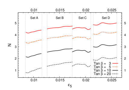
In Fig. 11, we depict the eigenvalues of , as a function of , for the input orbifold parameter sets A, B, C and D. Leading to this figure we have assumed , , a regime of , and a normal hierarchy for the light neutrino spectrum, namely
| (83) |
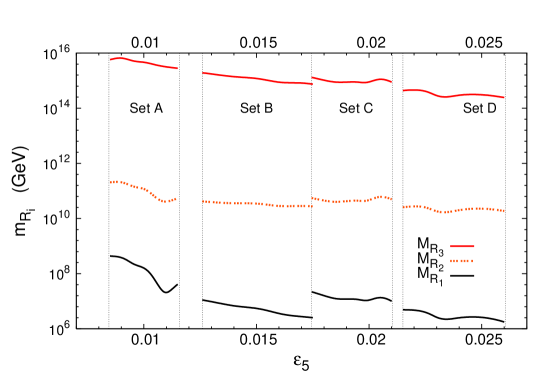
As can be seen from Fig. 11, the orbifold
structure would indeed suggest the existence of heavy Majorana
neutrinos, whose masses would lie in the GeV and
GeV ranges for the lightest and heaviest states,
respectively.
Naturally, the heavy spectrum strongly reflects the input
parameters, with the most important role being played by
, and the hierarchy of the light
neutrinos.
Essentially translates in an overall factor, and
having normal/inverted hierarchy or quasi-degenerate light neutrinos
mostly affects the pattern. On the other hand, the chosen
range can have a crucial impact: while values of
(as used for
Fig. 11) lead to masses in the
GeV range, larger values, close to 1, can even give rise to
masses as small as (TeV).
The phenomenological implications of the
latter regime would be extensive, and we do not address them
here.
Finally, and as an illustrative example, we present the complete matrix structure, for the orbifold set of parameters taken in Eq. (64), , , and the light-neutrino spectrum of Eq. (83):
| (84) |
Using this matrix one can check that both a high seesaw scale and additional mixings involving the right-handed neutrinos should be invoked in order to reproduce the correct neutrino masses and mixings. The eigenvalues for the Majorana mass matrix (which correspond to the masses of the heavy neutrinos) are
| (85) |
From these values one can see that, due to the mixing in the upper-left block matrix in Eq. (84), we encounter a very suppressed mass eigenvalue. For different regimes in the relevant parameters considered (, , and the light-neutrino mass spectrum) one can check that this eigenvalue may be even sufficiently small to lie at the TeV scale, being thus potentially detectable. The other eigenvalues, as can be seen in Fig. 11, remain always heavy, between and GeV.
Although phenomenological viable, these last implementation of a type-I seesaw is, as previously mentioned, neither related to the geometry of the orbifold, nor to the dynamics associated with FI breaking. In what follows, we pursue one final avenue, possibly leading to a more appealing seesaw realisation.
6.3 A viable seesaw from the FI breaking
As mentioned, a third possibility for reproducing the observed neutrino masses and mixings may be related with assuming a more complex FI breaking. Here, we briefly outline the idea, for the simplest case of one generation. Let us then assume that in addition to the and fields, which have the standard location
| (86) |
there are additional matter fields (triplets, doublet or singlets) , coupled to the fields which develop very large VEVs, thus inducing FI breaking. One can assume that these fields have the following assignments with respect to the first two sublattices:
| (87) |
The latter develop VEVs, , with GeV. In principle, one can also have the following terms in the superpotential
| (88) |
With the above proposed lattice assignments, and after FI breaking, this would lead to
| (89) |
In the basis defined by , one would then arrive at the following “mass matrix” (again neglecting family dependence as a first approach),
| (90) |
with eigenvalues given by
| (91) |
Further assuming that we are in the limit where is low (favoured from several arguments, as discussed throughout this work), is smaller than unity. In this limit, and given that , one would find
| (92) |
thus implying the presence of a term in the superpotential behaving like
| (93) |
with
| (94) |
In the superpotential involving the MSSM fields, the term in Eq. (93) would effectively generate a Majorana mass term for the neutrino field. Thus, an intermediate Majorana scale (lower than the FI breaking scale, and much heavier than the EW scale) would naturally appear, induced from the dynamics of FI breaking. Other mixings between and the remaining matter fields could in principle occur, but can be suppressed by some appropriate symmetry.
Whether or not such a FI-seesaw would indeed reproduce the correct three family neutrino masses and mixings is a question worth discussion. Additionally, one should also recall that the existence of heavy Majorana neutrinos, with possibly complex Yukawa couplings (for a discussion of how to implement CP violation in this class of orbifold constructions, see Ref. [56]), offers the possibility of generating the observed baryon asymmetry of the Universe from thermal leptogenesis [68]. This can be an involved question, given that as seen in Section 6.2, the scale of the lightest right-handed neutrino can range over several orders of magnitude. These two issues, and others like the collider signatures of potentially light Majorana neutrinos will be the subject of a subsequent analysis.
7 Conclusions
In this study we have aimed at completing the analysis of the phenomenological viability of abelian orbifold compactifications with two Wilson lines. This class of models, which naturally includes three families of fermions and Higgs fields, offers the possibility of obtaining realistic fermion masses and mixings, entirely at the renormalisable level. The Yukawa couplings arise from the geometrical configuration of the orbifold, and since they are explicitly calculable, one obtains a solution to the flavour problem of the SM and MSSM.
Successfully reproducing the observed pattern of quark masses and mixings already severely constrains the orbifold parameters. Furthermore, the presence of six Higgs doublets poses potential problems regarding tree-level FCNCs, which can nevertheless be avoided with a fairly light Higgs boson spectrum.
Here we have addressed in detail the implications of this class of orbifold compactifications for the lepton sector. Regarding the charged leptons, we verified that the still unconstrained orbifold parameters could easily account for the observed spectrum. Moreover, and even though one is equally likely to encounter tree-level contributions to three-body LFV decays, the typical choices of Higgs soft-breaking masses (taken as to comply with the bounds on neutral meson FCNC) ensure that the predicted BRs lie several orders of magnitude below the experimental bounds.
Regarding the neutrino sector, the orbifold model offers multiple possibilities. Albeit promising, we verified that the hypothesis of strictly Dirac neutrinos requires that the fields entering the FI breaking should have extremely hierarchical VEVs, forcing to call upon effective non-renormalisable couplings. Implementing a type-I seesaw mechanism via extra singlet fields whose interactions are dictated by the orbifold configuration reveals to be equally difficult. Complying with the measured mass squared differences favours VEVs for the Majorana singlets far higher than for the other fields. This again introduced the need to interpret these fields as effective non-renormalisable fields. Additionally, this mechanism fails in accommodating the current bounds on the neutrino mixing angles.
The need of additional mixing involving the Majorana singlet sector, and of an intermediate scale of about GeV motivated us to consider a third possibility. We have thus assumed that the smallness of the light neutrino masses is indeed explained by a type-I seesaw mechanism, where nor the scale, nor the mixings of the heavy singlets are predicted by the orbifold. In this case we verified that neutrino masses and mixings can be easily obtained, with a particularly interesting possibility which is that of a TeV-mass Majorana singlet.
In spite of the latter, it would be theoretically more appealing and consistent to have neutrino masses and mixings strictly from geometrical argumentations and/or from FI breaking. We pursued this challenging possibility, finding that in the simplest one-generation case, a slightly more involved FI breaking can indeed give rise to a Majorana mass term, with a scale far lower than that of FI breaking, and much higher than the EW scale.
This final possibility is definitely worth further investigation. In addition, one can also investigate the viability of generating the observed baryon asymmetry of the Universe from thermal leptogenesis. Having Majorana singlets that can be (although not necessarily) as light as the EW scale, also poses interesting scenarios regarding collider signatures.
8 Acknowledgements
N. Escudero is deeply grateful to the members of the Laboratoire de Physique Théorique, Université de Paris -Sud XI, for their kind hospitality in Orsay during the final stages of this work. He also thanks E. Arganda for useful discussions.
The work of N. Escudero is supported by the “Consejería de Educación de la Comunidad de Madrid - FPI Program” and “European Social Fund”. The work of C. Muñoz is supported in part by the Spanish DGI of the MEC under Proyectos Nacionales FPA2006-05423 and FPA2006-01105, by the European Union under the RTN program MRTN-CT-2004-503369, and by the Comunidad de Madrid under Proyecto HEPHACOS, Ayudas de I+D S-0505/ESP-0346. The work of A. M. Teixeira is supported by the French ANR project PHYS@COL&COS.
References
- [1] S. Eidelman et al. [Particle Data Group], “Review of particle physics,” Phys. Lett. B 592 (2004) 1.
- [2] M. C. Gonzalez-Garcia and M. Maltoni, “Phenomenology with Massive Neutrinos,” arXiv:0704.1800 [hep-ph].
- [3] M. Maltoni, T. Schwetz, M. A. Tortola and J. W. F. Valle, “Status of global fits to neutrino oscillations,” New J. Phys. 6, 122 (2004) [arXiv:hep-ph/0405172].
- [4] A. Strumia and F. Vissani, “Implications of neutrino data circa 2005,” Nucl. Phys. B 726, 294 (2005) [arXiv:hep-ph/0503246].
- [5] G. L. Fogli, E. Lisi, A. Marrone and A. Palazzo, “Global analysis of three-flavor neutrino masses and mixings,” Prog. Part. Nucl. Phys. 57, 742 (2006) [arXiv:hep-ph/0506083].
- [6] D. J. Gross, J. A. Harvey, E. J. Martinec and R. Rohm, “The heterotic string”, Phys. Rev. Lett. 54 (1985) 502; “Heterotic string theory. 1. The free heterotic string”, Nucl. Phys. B 256 (1985) 253; “Heterotic string theory. 2. The interacting heterotic string”, Nucl. Phys. B 267 (1986) 75.
- [7] L. J. Dixon, J. A. Harvey, C. Vafa and E. Witten, “Strings on orbifolds. 1”, Nucl. Phys. B 261 (1985) 678; “Strings on orbifolds. 2”, Nucl. Phys. B 274 (1986) 285.
- [8] L. E. Ibáñez, H. P. Nilles and F. Quevedo, “Orbifolds and Wilson lines”, Phys. Lett. B 187 (1987) 25.
- [9] L. E. Ibáñez, J. E. Kim, H. P. Nilles and F. Quevedo, “Orbifold compactifications with three families of ”, Phys. Lett. B 191 (1987) 282.
- [10] D. Bailin, A. Love and S. Thomas, “A three generation orbifold compactified superstring model with realistic gauge group”, Phys. Lett. B 194 (1987) 385.
- [11] L. E. Ibáñez, J. Mas, H. P. Nilles and F. Quevedo, “Heterotic strings in symmetric and asymmetric orbifold backgrounds”, Nucl. Phys. B 301 (1988) 157.
- [12] J. A. Casas, E. K. Katehou and C. Muñoz, “U(1) charges in orbifolds: anomaly cancellation and phenomenological consequences”, Nucl. Phys. B 317 (1989) 171.
- [13] A. Font, L. E. Ibáñez, H. P. Nilles and F. Quevedo, “Degenerate orbifolds”, Nucl. Phys. B 310 (1988) 109.
- [14] J. E. Kim, “The strong CP problem in orbifold compactifications and an model”, Phys. Lett. B 207 (1988) 434.
- [15] J. A. Casas and C. Muñoz, “Three generation orbifold models through Fayet-Iliopoulos terms”, Phys. Lett. B 209 (1988) 214.
- [16] J. A. Casas and C. Muñoz, “Three generation models from orbifolds”, Phys. Lett. B 214 (1988) 63.
- [17] A. Font, L. E. Ibáñez, H. P. Nilles and F. Quevedo, “Yukawa couplings in degenerate orbifolds: towards a realistic superstring”, Phys. Lett. B 210 (1988) 101 [Erratum-ibid. B 213 (1988) 564].
- [18] J. A. Casas and C. Muñoz, “Yukawa couplings in orbifold models”, Phys. Lett. B 212 (1988) 343.
- [19] J. A. Casas and C. Muñoz, “Restrictions on realistic superstring models from renormalization group equations”, Phys. Lett. B 214 (1988) 543.
- [20] A. Font, L. E. Ibáñez, F. Quevedo and A. Sierra, “The construction of ’realistic’ four-dimensional strings through orbifolds”, Nucl. Phys. B 331 (1990) 421.
- [21] J. A. Casas M. Mondragon and C. Muñoz, “Reducing the number of candidates to standard model in the orbifold”, Phys. Lett. B 230 (1989) 63.
- [22] Y. Katsuki, Y. Kawamura, T. Kobayashi, N. Ohtsubo, Y. Ono and K. Tanioka, “ orbifold models”, Nucl. Phys. B 341 (1990) 611.
- [23] H. B. Kim and J. E. Kim, “An orbifold compactification with three families from twisted sectors”, Phys. Lett. B 300 (1993) 343 [arXiv:hep-ph/9212311].
- [24] G. Aldazabal, A. Font, L. E. Ibáñez and A. M. Uranga, “Building GUTs from strings”, Nucl. Phys. B 341 (1990) 611 [arXiv:hep-th/9508033].
- [25] J. Giedt, “Spectra in standard-like orbifold models”, Annals Phys. 297 (2002) 67 [arXiv:hep-th/0108244].
- [26] C. Muñoz, “A kind of prediction from superstring model building”, JHEP 0112 (2001) 015 [arXiv:hep-ph/0110381].
- [27] T. Kobayashi, S. Raby, R.-J. Zhang, “Searching for realistic 4d string models with a Pati-Salam symmetry: Orbifold grand unified theories from heterotic string compactification on a orbifold”, Nucl. Phys. B704 (2005) 3 [arXiv:hep-ph/0409098].
- [28] J. Giedt, G. L. Kane, P. Langacker and B. D. Nelson, “Massive neutrinos and (heterotic) string theory,” Phys. Rev. D 71 (2005) 115013 [arXiv:hep-th/0502032].
- [29] T. Kobayashi and C. Muñoz, “More about soft terms and FCNC in realistic string constructions”, JHEP 0601 (2006) 044 [arXiv:hep-ph/0508286].
- [30] W. Buchmuller, K. Hamaguchi, O. Lebedev, M. Ratz, “Supersymmetric standard model from the heterotic string”, Phys. Rev. Lett. 96 (2006) 121602 [arXiv:hep-ph/0511035]; “Supersymmetric standard model from the heterotic string (II)”, Nucl. Phys. B785 (2007) 149 [arXiv:hep-th/0606187].
- [31] J.E. Kim and B. Kyae, “String MSSM through flipped SU(5) from orbifold”, arXiv:hep-th/0608085; “Flipped SU(5) from orbifold with Wilson line”, Nucl. Phys. B770 (2007) 47 [arXiv:hep-th/0608086].
- [32] O. Lebedev, H.P. Nilles, S. Raby, S. Ramos-Sánchez, M. Ratz, P.K. Vaudrevange and A. Wingerter, “A mini-landscape of exact MSSM spectra in heterotic orbifolds”, Phys. Lett. B645 (2007) 88 [arXiv:hep-th/0611095]; “Low energy supersymmetry from the heterotic landscape”, Phys. Rev. Lett. 98 (2007) 181602 [arXiv:hep-th/0611203]; “The heterotic road to the MSSM with R parity”, arXiv:0708.2691[hep-th].
- [33] I-W. Kim, J.E. Kim and B. Kyae, “Harmless R-parity violation from compactification of heterotic string”, Phys. Lett. B647 (2007) 275 [arXiv:hep-ph/0612365].
- [34] J.E. Kim, J.-H. Kim and B. Kyae, “Superstring standard model from orbifold compactification with and without exotics, and effective R-parity”, JHEP 0706 (2007) 034 [arXiv:hep-ph/0702278].
- [35] W. Buchmuller, K. Hamaguchi, O. Lebedev, S. Ramos-Sánchez, M. Ratz, “Seesaw neutrinos from the heterotic string”, arXiv:hep-th/0703078.
- [36] E. Witten, “Some properties of O(32) superstrings”, Phys. Lett. B 149 (1984) 351.
- [37] M. Dine, N. Seiberg and E. Witten, “Fayet-Iliopoulos terms in string theory”, Nucl. Phys. B 289 (1987) 589.
- [38] J. J. Atick, L. J. Dixon and A. Sen, “String calculation of Fayet-Iliopoulos D terms in arbitrary supersymmetric compactifications”, Nucl. Phys. B 292 (1987) 109.
- [39] M. Dine, I. Ichinose and N. Seiberg, “F terms and D terms in string theory”, Nucl. Phys. B 293 (1987) 253.
- [40] S. Hamidi and C. Vafa, “Interactions on orbifolds”, Nucl. Phys. B 279 (1987) 465.
- [41] L. J. Dixon, D. Friedan, E. J. Martinec and S. H. Shenker, “The conformal field theory of orbifolds”, Nucl. Phys. B 282 (1987) 13.
- [42] L. E. Ibáñez, “Hierarchy of quark-lepton masses in orbifold superstring compactification”, Phys. Lett. B 181 (1986) 269.
- [43] J. A. Casas and C. Muñoz, “Fermion masses and mixing angles: a test for string vacua”, Nucl. Phys. B 332 (1990) 189 [Erratum-ibid. B 340 (1990) 280].
- [44] J. A. Casas, F. Gómez and C. Muñoz, “Fitting the quark and lepton masses in string theories”, Phys. Lett. B 292 (1992) 42 [arXiv:hep-th/9206083].
- [45] J. A. Casas, F. Gómez and C. Muñoz, “World sheet instanton contribution to Yukawa couplings”, Phys. Lett. B 251 (1990) 99.
- [46] T. T. Burwick, R. K. Kaiser and H. F. Muller, “General Yukawa couplings of strings on orbifolds”, Nucl. Phys. B 355 (1991) 689.
- [47] T. Kobayashi and N. Ohtsubo, “Geometrical aspects of orbifold phenomenology”, Int. J. Mod. Phys. A 9 (1994) 87.
- [48] J. A. Casas, F. Gómez and C. Muñoz, “Complete structure of Yukawa couplings,” Int. J. Mod. Phys. A 8 (1993) 455 [arXiv:hep-th/9110060].
- [49] S. A. Abel and C. Muñoz, “Quark and lepton masses and mixing angles from superstring constructions,” JHEP 0302 (2003) 010 [arXiv:hep-ph/0212258].
- [50] P. Ko, T. Kobayashi and J. h. Park, “Quark masses and mixing angles in heterotic orbifold models”, Phys. Lett. B 598 (2004) 263 [arXiv:hep-ph/0406041].
- [51] P. Ko, T. Kobayashi and J. h. Park, “Lepton masses and mixing angles from heterotic orbifold models”, Phys. Rev. D 71 (2005) 095010 [arXiv:hep-ph/0503029].
- [52] H. Georgi and D. V. Nanopoulos, “Suppression of flavor changing effects from neutral spinless meson exchange in gauge theories”, Phys. Lett. B 82 (1979) 95.
- [53] B. McWilliams and L. F. Li, “Virtual Effects Of Higgs Particles,” Nucl. Phys. B 179 (1981) 62.
- [54] O. Shanker, “Flavor violation, scalar particles and leptoquarks,” Nucl. Phys. B 206 (1982) 253.
- [55] N. Escudero, C. Muñoz and A. M. Teixeira, “FCNCs in supersymmetric multi-Higgs doublet models,” Phys. Rev. D 73 (2006) 055015 [arXiv:hep-ph/0512046].
- [56] N. Escudero, C. Muñoz and A. M. Teixeira, “Phenomenological viability of orbifold models with three Higgs families,” JHEP 0607 (2006) 041 [arXiv:hep-ph/0512301].
- [57] Z. Maki, M. Nakagawa and S. Sakata, “Remarks on the unified model of elementary particles,” Prog. Theor. Phys. 28 (1962) 870.
- [58] B. Pontecorvo, “Mesonium and antimesonium,” Sov. Phys. JETP 6 (1957) 429 [Zh. Eksp. Teor. Fiz. 33 (1957) 549].
- [59] P. Minkowski, “ e at a rate of one out of 1-billion muon decays?,” Phys. Lett. B 67 (1977) 421; M. Gell-Mann, P. Ramond and R. Slansky, in Complex spinors and Unified Theories eds. P. Van. Nieuwenhuizen and D. Z. Freedman, Supergravity (North-Holland, Amsterdam, 1979), p.315 [Print-80-0576 (CERN)]; T. Yanagida, in Proceedings of the Workshop on the Unified Theory and the Baryon Number in the Universe, eds. O. Sawada and A. Sugamoto (KEK, Tsukuba, 1979), p.95; S. L. Glashow, in Quarks and Leptons, eds. M. Lévy et al. (Plenum Press, New York, 1980), p.687; R. N. Mohapatra and G. Senjanović, “Neutrino mass and spontaneous parity nonconservation,” Phys. Rev. Lett. 44 (1980) 912; J. Schechter and J. W. F. Valle, “Neutrino masses in theories,” Phys. Rev. D 22 (1980) 2227; “Neutrino decay and spontaneous violation of lepton number,” Phys. Rev. D 25 (1982) 774.
- [60] M. Drees, “Supersymmetric models with extended Higgs sector,” Int. J. Mod. Phys. A 4 (1989) 3635.
- [61] E. Arganda and M. J. Herrero, “Testing supersymmetry with lepton flavor violating tau and mu decays,” Phys. Rev. D 73 (2006) 055003 [arXiv:hep-ph/0510405].
- [62] S. Antusch, E. Arganda, M. J. Herrero and A. M. Teixeira, “Impact of theta(13) on lepton flavour violating processes within SUSY seesaw,” JHEP 0611 (2006) 090 [arXiv:hep-ph/0607263].
- [63] E. Arganda, M. J. Herrero and A. M. Teixeira, “ conversion in nuclei within the CMSSM seesaw: universality versus non-universality”, arXiv:0707.2955 [hep-ph].
- [64] U. Bellgardt et al. [SINDRUM Collaboration], “Search For The Decay Mu+ E+ E+ E-”, Nucl. Phys. B 299 (1988) 1.
- [65] B. Aubert et al. [BABAR Collaboration], “Search for lepton flavor violation in the decay tau- l- l+ l-”, Phys. Rev. Lett. 92 (2004) 121801 [arXiv:hep-ex/0312027].
- [66] A. G. Akeroyd et al. [SuperKEKB Physics Working Group], “Physics at super B factory”, [arXiv:hep-ex/0406071].
- [67] D. Ng and J. N. Ng, “Can - e conversion in nuclei be a good probe for lepton number violating Higgs couplings?”, Phys. Lett. B 320 (1994) 181 [arXiv:hep-ph/9308352].
- [68] M. Fukugita and T. Yanagida, “Baryogenesis without Grand Unification”, Phys. Lett. B 174 (1986) 45.