Asymptotics of eigenfunctions on plane domains

Abstract.

We consider a family of domains $(\Omega_{N})_{N>0}$ obtained by attaching an $N\times 1$ rectangle to a fixed set $\Omega_{0}=\{(x,y):\,0<y<1,\,-\phi(y)<x<0\}$, for a Lipschitz function $\phi\geq 0$. We derive full asymptotic expansions, as $N\to\infty$, for the $m$th Dirichlet eigenvalue (for any fixed $m\in\mathbb{N}$) and for the associated eigenfunction on $\Omega_{N}$. The second term involves a scattering phase arising in the Dirichlet problem on the infinite domain $\Omega_{\infty}$. We determine the first variation of this scattering phase, with respect to $\phi$, at $\phi\equiv 0$. This is then used to prove sharpness of results, obtained previously by the same authors, about the location of extrema and nodal line of eigenfunctions on convex domains.

1. Introduction

For a Lipschitz function $\phi:[0,1]\to[0,\infty)$ and for $N\in[0,\infty]$ consider the plane domain (see Figure 1)

(1.1) $$\Omega_{N}=\{(x,y)\in\mathbb{R}^{2}:0<y<1,\,-\phi(y)<x<N\}$$

and the eigenvalue problem for the Dir chlet Laplacian on $\Omega_{N}$:

$$(\Delta+\mu)u =0\quad\text{on }\Omega_{N}$$

$$u =0\quad\text{at }\partial\Omega_{N}.$$

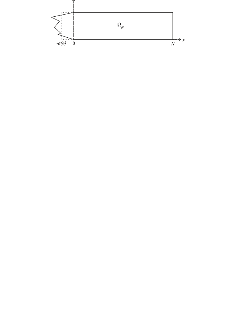
Figure 1. The domain $\Omega_{N}$

For $N<\infty$ let $\mu_{1}(\Omega_{N})<\mu_{2}(\Omega_{N})\leq\dots$ be the eigenvalues, counted with multiplicities. The object of this paper is to study, for fixed $m\in\mathbb{N}$, the asymptotic behavior of $\mu_{m}(\Omega_{N})$ and of the associated eigenfunctions, as $N\to\infty$. This will then be used to answer some questions left open in our study (see [8, 4, 5]) of the first and the second eigenfunction on general plane convex domains.

Our first main theorem is:

Theorem 1.

There is a number $a(\phi)\in[0,\max\phi]$ such that for each $m\in\mathbb{N}$ the $m$th Dirichlet eigenvalue of $\Omega_{N}$ satisfies

(1.2) $$\mu_{m}(\Omega_{N})=\pi^{2}+\frac{m^{2}\pi^{2}}{(N+a(\phi))^{2}}+O(N^{-5}),\quad N\to\infty.$$

In particular, the eigenvalues $\mu_{1},\dots,\mu_{m}$ of $\Omega_{N}$ are simple for $N$ sufficiently large. The suitably rescaled eigenfunction $u_{m}$ satisfies, for all multiindices $\alpha$,

(1.3) $$\sup_{x>3\log N}|D^{\alpha}\left(u_{m}(x,y)-\sin m\pi\frac{x+a(\phi)}{N+a(\phi)}\,\sin\pi y\right)|=O(N^{-3}),$$

(1.4) $$\sup_{x\leq 3\log N}|u_{m}(x,y)|=O(N^{-1}{\log N}).$$

The constants in the error terms only depend on $k,\ \alpha$ and $\max\phi$.

Thus, the spectral data are very close to the data obtained on the rectangle $[-a(\phi),N]\times[0,1]$. In fact, we will get complete asymptotic expansions for the eigenvalue and the eigenfunction and also much more precise information about the eigenfunction for small values of $x$, see Remark 12 and Theorem 15 (in connection with (3.14)).

The number $a(\phi)$ is closely related to a scattering phase in an associated non-compact problem, see Section 2, in particular Remark 8. Therefore, its dependence on $\phi$ is very subtle. Our second main theorem gives a perturbation analysis of $a(\phi)$ around $\phi\equiv 0$:

Theorem 2.

Fix a Lipschitz function $\phi:[0,1]\to[0,\infty)$. Then, as $\epsilon\to 0$,

(1.5) $$a(\epsilon\phi)=2\epsilon\int_{0}^{1}\phi(y)(\sin\pi y)^{2}\,dy+O(\epsilon^{2}).$$

As already mentioned, one motivation for the present study is to complement the results about the first and second eigenfunction $u_{1}$, $u_{2}$ on a plane convex domain $\Omega$ obtained in [8, 5]. In these papers we considered the maximum of $u_{1}$ (which is w.l.o.g. assumed positive) and the nodal line of $u_{2}$, and a central goal was to localize these objects in terms of corresponding objects for eigenfunctions of an associated ordinary differential operator. To state this more precisely, we first normalize $\Omega$ by a rotation and a dilation so that among all projections of $\Omega$ onto lines the projection onto the $y$-axis has shortest possible length and this length equals one. Let $\pi(x,y)=x$ be the projection map to the $x$ axis. Let $I=\pi(\Omega)$ and $h:I\to(0,\infty)$ be the ’height function’ of $\Omega$, that is,

$$h(x)=\text{length of the interval }\pi^{-1}(\{x\})\cap\Omega.$$

Let $\phi_{1},\phi_{2}$ be the first and second eigenfunction of the Schrödinger operator $-\dfrac{d^{2}}{dx^{2}}+\dfrac{\pi^{2}}{h(x)^{2}}$ on $I$, with Dirichlet boundary conditions (defined in terms of the variational principle on $H^{1}_{0}(I)$).

Theorem 3 ([8, 5]).

Let the domain $\Omega$ be normalized as above and let $h:I\to(0,\infty)$ be its height function. Denote by $\mathcal{M}$ the set where $u_{1}$ achieves its maximum, by $\mathcal{N}=u_{2}^{-1}(0)$ the nodal line, and let $\{m\}$ and $\{n\}$ be the corresponding sets for $\phi_{1},\phi_{2}$.

There is an absolute constant $C$ so that

(1.6) $$\pi(\mathcal{M})\subset[m-C,m+C],\qquad\pi(\mathcal{N})\subset[n-C,n+C].$$

Actually, $\mathcal{M}$ consists of a single point, by a well-known argument using the convexity of $\Omega$. Also, the uniqueness of the point $m$ follows by standard arguments from the convexity of $h$, while the uniqueness of $n$ is a general fact from Sturm theory.

A consequence of the theorem is that, while clearly the interval $I$ and the function $h$ do not determine $\Omega$ uniquely, these data do determine the location of the distinctive features of $u_{1},u_{2}$ up to a bounded error, uniformly for all domains normalized as above (in particular, uniformly as $\lvert I\rvert\to\infty$).

The question left open in [8, 5] is whether the result (1.6) is sharp in order of magnitude as $\lvert I\rvert\to\infty$. We will derive from Theorems 1 and 2 that this is in fact true:

Theorem 4.

There is $c>0$ and, for each $N^{\prime}>0$, a pair of domains $\Omega,\tilde{\Omega}$, normalized as above and with $\pi(\Omega)=\pi(\tilde{\Omega})$ of length $N^{\prime}$ and with the same height function, such that

(1.7) $$\operatorname{dist}(\pi(\mathcal{M}),\pi(\tilde{\mathcal{M}}))>c,\qquad\operatorname{dist}(\pi(\mathcal{N}),\pi(\tilde{\mathcal{N}}))>c.$$

See Figure 2 at the end of the paper. This should be put in contrast with the main result of [4] which states that the length of the interval $\pi(\mathcal{N})$ is not bounded away from zero, but actually bounded above by $C/\lvert I\rvert$, for an absolute constant $C$.

Our approach to Theorem 1 is via the method of matched asymptotic expansions. This is carried out in Section 3. Here one has to deal with two limiting problems: The first one is the equation $(-\frac{d^{2}}{d\xi^{2}}+\lambda)\psi(\xi)=0$ on the interval $[0,1]$, and is easily solved explicitly. The second one is the equation $(\Delta+\pi^{2})U=0$ on the unbounded domain $\Omega_{\infty}$; we need some results about generalized eigenfunctions on $\Omega_{\infty}$, which are known from scattering theory. For completeness we give a direct derivation of what we need in Section 2. Here, the quantity $a(\phi)$ arises. Theorem 2 is proved in Section 4 and Theorem 3 in Section 5.

The asymptotic behavior of spectral quantities on degenerating spaces similar to the family $(\Omega_{N})_{N>0}$ has been studied by many authors in different contexts. Regarding invariants involving all the eigenvalues (like the determinant of the Laplacian) we only mention [7], [11] and [12]. Our results are also related to the investigations of so-called thick graphs (or graph-like thin manifolds): When rescaling $\Omega_{N}$ by a factor $1/N$, one obtains a domain which is a $1/2N$-neighborhood of a unit interval, except for a fixed (scaled) perturbation at the ends of the interval. Instead of the interval (considered as a graph with two nodes and one edge of length one connecting them) one may consider more general embedded graphs, and their $\epsilon$-neighborhoods (or more general ’$\epsilon$-thin’ manifolds modeled on the graph). The convergence of eigenvalues, as $\epsilon$ tends to zero, to spectral data on the graph itself (then sometimes called a ’quantum graph’) was studied in [9, 13, 1], for the Neumann and closed problems. The Dirichlet and mixed boundary value problems are studied in the preprints [3] (where it is also proved that the asymptotic series constructed in this paper converge) and [10], by different methods than the one used in this paper. The Dirichlet problem is more difficult to handle since the dependence on the counting parameter $k$ appears in a lower order term, cf. equation (1.2). While in these papers the graph edges are always straight lines, the case of a curved line (but without the perturbation at the end) is considered in [2], where a nodal line theorem is proved.

2. Eigenfunctions on the infinite domain

In this section we prove the results about generalized eigenfunctions on $\Omega_{\infty}$ which will be needed in the proof of Theorem 1. Since, for any $m$, the $m$th eigenvalue on $\Omega_{N}$ converges to $\pi^{2}$ as $N\to\infty$ (by domain comparison), we need to consider the spectral value $\pi^{2}$, which is the bottom of the continuous spectrum of $-\Delta_{\text{Dir}}$ on $\Omega_{\infty}$.

Proposition 5.

1. There is a unique function $U$ on $\Omega_{\infty}$ satisfying

   $$(\Delta+\pi^{2})U =0\quad\text{on }\Omega_{\infty}$$

   (2.1) $$U =0\quad\text{at }\partial\Omega_{\infty}$$

   $$U-x\sin\pi y$$ is bounded.

2. For this function $U$ define

   (2.2) $$a(\phi)=2\int_{0}^{1}U(0,y)\sin\pi y\,dy.$$

   Then

   (2.3) $$U(x,y)=(x+a(\phi))\sin\pi y+r(x,y)$$

   where the remainder decays exponentially as $$x\to\infty$$, more precisely,

   (2.4) $$r(x,y)=\sum_{k=2}^{\infty}r^{(k)}(x)\sin k\pi y,\quad|d_{x}^{p}r^{(k)}(x)|\leq C_{p}e^{-kx/2}\ \forall p,k.$$

   Here, $C_{p}$ is independent of $k$ and $x$ and is bounded in terms of $\max\phi$.

Note that in the special case where $\phi$ is a constant $A$, the function $U$ is simply $(x+A)\sin\pi y$, so $a(\phi)=A$. Therefore, for general $\phi$, the number $a(\phi)$ tells how much the ’standard’ problem, with $\Omega_{\infty}=[0,\infty)\times[0,1]$, has to be shifted so that its first (generalized) eigenfunction coincides asymptotically with that of the ’perturbed’ problem. See also Remark 8.

For simplicity, we assume all functions are real valued. Basic to all considerations is the explicit form of solutions of the homogeneous equation:

Lemma 6.

Assume $u$ solves $(\Delta+\pi^{2})u=0$ in $x\geq x_{0},\ y\in(0,1)$, vanishes for $y=0$ and $y=1$ and has at most polynomial growth as $x\to\infty$. Then

(2.5) $$u(x,y)=(A_{1}+B_{1}x)\sin\pi y+\sum_{k=2}^{\infty}A_{k}e^{-\sqrt{k^{2}-1}\pi x}\sin k\pi y\quad\text{ for }x\geq x_{0},$$

for certain numbers $A_{k}$, $B_{1}$.

Proof.

$u$ is smooth, so for each fixed $x$ it is the sum of its Fourier series, $u(x,y)=\sum_{k=1}^{\infty}u_{k}(x)\sin k\pi y$, where $u_{k}(x)=2\int_{0}^{1}u(x,y)\sin k\pi y\,dy$. From $(\Delta+\pi^{2})u=0$ one gets $u_{k}^{\prime\prime}+(1-k^{2})\pi^{2}u_{k}=0$. This gives $u_{1}(x)=A_{1}+B_{1}x$ and $u_{k}(x)=A_{k}e^{-\sqrt{k^{2}-1}\pi x}+B_{k}e^{\sqrt{k^{2}-1}\pi x}$ for $k\geq 2$. Since $u$ is polynomially bounded, so is $u_{k}$, and therefore $B_{k}=0$ for $k\geq 2$. ∎

Lemma 7.

Let $w\in L^{2}(\Omega_{\infty})$ be supported in $\Omega_{1}$.

1. If $u\in H^{1}(\Omega_{\infty})$ solves

   $$(\Delta+\pi^{2})u =w\quad\text{on }\Omega_{\infty},$$

   (2.6) $$u =0\quad\text{at }\partial\Omega_{\infty},$$

   $$u$$ is bounded

   then

   (2.7) $$\|u\|^{2}_{H^{1}(\Omega_{1})}\leq-C(u,w)$$

   where $C$ is bounded in terms of the maximum of $\phi$.

2. Problem (2.6) has a unique solution $u$.

Proof.

(1) We integrate by parts and use the support assumption to obtain

(2.8) $$-(u,w)=-\int_{\Omega_{1}}u(\Delta+\pi^{2})u=-\int_{\partial\Omega_{1}}uu_{n}+\int_{\Omega_{1}}|\nabla u|^{2}-\pi^{2}\int_{\Omega_{1}}u^{2}$$

where $u_{n}$ is the outward normal derivative. Therefore, it is sufficient to prove the following two facts:

(2.9) $$\text{If }u\text{ is as in \eqref{GJ.91} and bounded then }\int_{0}^{1}u(x_{0},y)\frac{\partial u(x_{0},y)}{\partial x}\,dy\leq 0.$$

(2.10) $$\text{If }u\in H^{1}(\Omega_{1})\text{ and }u=0\text{ on }\partial\Omega_{1}\setminus\{x=1\}\text{ then }\int_{\Omega_{1}}|\nabla u|^{2}-\pi^{2}\int_{\Omega_{1}}u^{2}\geq c\|u\|^{2}_{H^{1}(\Omega_{1})}.$$

To prove (2.9), observe that $B_{1}=0$ in (2.5) since $u$ is bounded. Therefore, $\int_{0}^{1}u(x_{0},y)\partial_{x}u(x_{0},y)\,dy=-\pi/2\sum_{k=2}^{\infty}A_{k}^{2}\sqrt{k^{2}-1}\exp(-2\sqrt{k^{2}-1}\pi x_{0})\leq 0$.

To prove (2.10), consider the domain $\tilde{\Omega}$ which is the union of $\Omega_{1}$, the boundary piece $\{1\}\times(0,1)$, and the reflection of $\Omega_{1}$ across this boundary. Since $\tilde{\Omega}\subset(-A,A)\times(0,1)$ for some $A$, the first Dirichlet eigenvalue of $\tilde{\Omega}$ is strictly bigger than $\pi^{2}$, so it equals $(\pi^{2}+c)/(1-c)$ for some $c>0$. The function on $\tilde{\Omega}$ which equals $u$ for $x\leq 1$ and is symmetric with respect to the line $\{x=1\}$ is in $H^{1}_{0}(\tilde{\Omega})$, so we can use it as test function and obtain $(1-c)\int_{\Omega_{1}}|\nabla u|^{2}\geq(\pi^{2}+c)\int_{\Omega_{1}}u^{2}$, which implies (2.10). In this proof $A$ and therefore $c$ only depend on $\max\phi$.

(2) Uniqueness is clear from 1. To prove existence, we reduce to a compact problem. Define ’Dirichlet-to-Neumann operators’ $N_{1},N_{\infty}$, acting on functions on $S=\{1\}\times(0,1)$, as follows: Given $f\in H^{1}_{0}(S)\cap H^{2}(S)$, let $v_{1},v_{\infty}$ be the solutions of $(\Delta+\pi^{2})v=0$ on $\Omega_{1}$, $D=(1,\infty)\times(0,1)$ respectively, with boundary values $f$ at $S$ and zero elsewhere, and $v_{\infty}$ bounded. Existence and uniqueness follows for $v_{1}$ from the fact that the first Dirichlet eigenvalue of $\Omega_{1}$ is bigger than $\pi^{2}$, and for $v_{\infty}$ by explicit computation as in Lemma 6. Set $N_{1}f:=\partial v_{1}/\partial x_{|S}$ and $N_{\infty}f:=\partial v_{\infty}/\partial x_{|S}$. The restrictions exist and are in $H^{1}(S)$ since $v_{1},v_{\infty}$ are in $H^{5/2}$ near $S$ by standard regularity theory.

From (2.9) applied to $u=v_{\infty}$ we have $(N_{\infty}f,f)\leq 0$, and from (2.10) $(N_{1}f,f)=\int_{\partial\Omega_{1}}(v_{1})_{n}v_{1}=\int_{\Omega_{1}}|\nabla v_{1}|^{2}-\pi^{2}\int_{\Omega_{1}}v_{1}^{2}\geq c\|v_{1}\|^{2}_{H^{1}(\Omega_{1})}\geq\|f\|^{2}_{H^{1/2}(S)}$, so we obtain

(2.11) $$((N_{1}-N_{\infty})f,f)\geq c\|f\|^{2}_{H^{1/2}(S)},\quad f\in H^{1}_{0}(S)\cap H^{2}(S).$$

Along the same lines one sees that $(N_{1}f,g)\leq\|f\|_{H^{1/2}(S)}\|g\|_{H^{1/2}(S)}$ for $f,g\in H^{1/2}_{0}(S)$, and this shows that $N_{1}$ can be extended to a bounded operator $H_{0}^{1/2}(S)\to H^{-1/2}(S)$, and similarly for $N_{\infty}$. By approximation, (2.11) continues to hold for $f\in H^{1/2}_{0}(S)$. This shows that $N_{1}-N_{\infty}$ has closed range and therefore is surjective, for if $g\in H^{1/2}_{0}(S)$ is orthogonal to the range then applying (2.11) to $g$ implies $g=0$.

Now we find a solution $u$ of (2.6) as follows: Let $v$ be the unique solution of $(\Delta+\pi^{2})v=w$ on $\Omega_{1}$, $v_{|\partial\Omega_{1}}=0$, and define $f$ on $S$ by $(N_{1}-N_{\infty})f=-\partial v/\partial x_{|S}$. For $f$ find functions $v_{1},v_{\infty}$ as above. Define the function $u$ by $v+v_{1}$ on $\Omega_{1}$ and by $v_{\infty}$ on $D$; at $S$, $u$ has the value $f$ from the left and right, and $\partial u/\partial x$ is $\partial v/\partial x+N_{1}f$ from the left and $N_{\infty}f$ from the right, which are equal by construction. Therefore, $u$ is the desired solution. ∎

Proof of Proposition 5.

(1) Let $\psi(x)$ be a smooth function vanishing for $x\leq 0$ and equal to one for $x\geq 1$. Let $u$ be the solution of (2.6) with $w=-(\Delta+\pi^{2})(\psi(x)x\sin\pi y)$. Then $U=u+\psi(x)x\sin\pi y$ solves (2.1). From (2.7) we have $\lVert u\rVert_{H^{1}(\Omega_{1})}\leq C\lVert w\rVert_{L^{2}(\Omega_{1})}\leq C^{\prime}$ and therefore also

(2.12) $$\lVert U\rVert_{H^{1}(\Omega_{1})}\leq C,$$

with $C$ only depending on $\max\phi$. Uniqueness is clear from the uniqueness for $u$.

(2) Apply Lemma 6 to $U$ with $x_{0}=0$. Since $U-x\sin\pi y$ is bounded, we have $B_{1}=1$. Since, from (2.12) and the trace theorem, $\sum_{k=1}^{\infty}A_{k}^{2}=\frac{1}{2}\int_{0}^{1}U(0,y)^{2}\,dy\leq C\lVert U\rVert_{H^{1}(\Omega_{1})}^{2}\leq C^{\prime}$, this gives (2.3) and (2.4) with $a(\phi)=A_{1}$, and evaluating $\int_{0}^{1}U(0,y)\sin\pi y\,dy$ yields (2.2). ∎

Remark 8.

We explain the relation of $a(\phi)$ to the scattering phase. Standard scattering theory (see, for example, [6]) yields that for $s>0$ close to zero the equation $(\Delta+\pi^{2}+s^{2})E=0$, $E_{|\partial\Omega_{\infty}}=0$ has a unique polynomially bounded solution on $\Omega_{\infty}$ of the form

$$E_{s}=(e^{-isx}+S(s)e^{isx})\,\sin\pi y+r_{s}(x,y)$$

for some number $S(s)$ (the scattering matrix) and a remainder $r_{s}(x,y)$ of the form (2.4). The function $S$ extends holomorphically to a neighborhood of zero in $\mathbb{C}$ and is real and of modulus one for real argument, hence may be written $S(s)=e^{i\gamma(s)}$ for a holomorphic function $\gamma$, the scattering phase. $r_{s}$ is also holomorphic in $s$ and the estimates (2.4) are uniform in $s$ near zero, so one can take the limit $s\to 0$ to get a solution of $(\Delta+\pi^{2})U=0$. This solution is bounded, hence constant equal to zero by Proposition 5. Therefore $S(0)=-1$ and $r_{0}\equiv 0$. One can get a nontrivial solution by taking $\lim_{s\to 0}\frac{1}{s}E_{s}=\frac{d}{ds}_{|s=0}E_{s}$, and this has leading term $-2i(x+\gamma^{\prime}(0)/2)\sin\pi y$. Comparison with (2.3) then yields

(2.13) $$a(\phi)=\frac{1}{2}\gamma^{\prime}(0).$$

We will also need an extension of Proposition 5:

Lemma 9.

Assume $v$ is a smooth function on $\Omega_{\infty}$ which vanishes at $\partial\Omega_{\infty}$ and for $x\geq 0$ has the form

$$v(x,y)=p(x)\sin\pi y+r(x,y),$$

with $p$ a polynomial and $r$ satisfying the estimates (2.4).

Then any polynomially bounded solution of the problem

(2.14) $$\begin{split}(\Delta+\pi^{2})u&=v\quad\text{on }\Omega_{\infty}\\ u&=0\quad\text{at }\partial\Omega_{\infty}\end{split}$$

has the same form $u(x,y)=q(x)\sin\pi y+s(x,y)$, where $s$ satisfies the estimates (2.4) and

(2.15) $$q^{\prime\prime}=p.$$

Such solutions exist, and are unique up to adding multiples of $U$, where $U$ is defined in Proposition 5.

Proof.

Let $u$ be a solution of (2.14). Taking the Fourier decomposition of $u(x,\cdot)$ we get $u(x,y)=q(x)\sin\pi y+\sum_{k=2}^{\infty}s^{(k)}(x)\sin k\pi y$, and then (2.14) gives (2.15) and, for each $k\geq 2$,

(2.16) $$(d_{x}^{2}+1-k^{2})s^{(k)}=r^{(k)}.$$

For any initial condition $s^{(k)}(0)=a_{k}$, (2.16) has the unique polynomially bounded solution

(2.17) $$s^{(k)}(x)=a_{k}e^{-\alpha x}-\frac{1}{2\alpha}\int_{0}^{\infty}\left(e^{-\alpha|x-z|}-e^{-\alpha(x+z)}\right)r^{(k)}(z)\,dz$$

where $\alpha=\sqrt{k^{2}-1}$. Since $u$ is given and $s^{(k)}(x)=2\int_{0}^{1}u(x,y)\sin k\pi y\,dy$, we have $a_{k}=2\int_{0}^{1}u(0,y)\sin k\pi y\,dy$. An easy calculation shows $|d_{x}^{p}s^{(k)}(x)|\leq Ce^{-kx/2}$, and this proves the first claim.

To prove existence of a solution, choose $q_{0}$ satisfying $q_{0}^{\prime\prime}=p$, and a cutoff function $\chi$, equal to zero for $x\leq 1$ and to one for $x\geq 2$, and set $u_{0}(x,y)=\chi(x)\left(q_{0}(x)\sin\pi y+\sum_{k=2}^{\infty}s^{(k)}_{0}(x)\sin k\pi y\right)$. This is polynomially bounded. Then $u=u_{0}+h$ solves (2.14) iff $h$ solves $(\Delta+\pi^{2})h=v_{1}$, $h_{|\partial\Omega_{\infty}}=0$, where $v_{1}=v-(\Delta+\pi^{2})u_{0}$ is compactly supported. Lemma 7 guarantees the existence of a bounded solution $h$.

Uniqueness is clear from Lemma 6 and Proposition 5. ∎

3. Asymptotic expansions of eigenfunctions and eigenvalues

In order to prove Theorem 1 we use the idea of matched asymptotic expansions. The strategy is this: First, we make reasonable guesses about the asymptotic behavior, as $N\to\infty$, of the $m$th eigenvalue and of certain scaled limits of the eigenfunction. This leads to an ansatz in the form of formal asyptotic series in terms of powers of $1/N$, whose coefficients are undetermined numbers (for the eigenvalue) resp. functions (for the eigenfunction). The eigenvalue equation, the boundary condition and the condition that the various scaled limits must fit together (’match’) in the transition region between different scaling regimes, yield a recursive system of equations for these coefficients. This system has a unique solution (Proposition 10). Given any approximation order, one then obtains a candidate for an approximate eigenvalue (by truncating the formal series), and also for an approximate eigenfunction, which is obtained by a suitable patching of the data from the different scaling regimes. These candidates satisfy the eigenvalue equation with a small error (Proposition 13), and from this we derive that they are close to actual eigenvalues. A domain comparison yields an a priori estimate on the actual eigenvalues, and this allows to conclude that all actual eigenvalues are obtained in this way, as well as a lower bound on the spectral gap. The spectral gap estimate then implies that the approximate eigenfunctions are close to actual eigenfunctions (Theorem 15). Using this explicit information, it is easy to derive Theorem 1.

3.1. The ansatz, formal eigenvalue and eigenfunction

Fix an integer $m\geq 1$. We want to find the $m$th eigenvalue and eigenfunction of $\Omega_{N}$, asymptotically as $N\to\infty$. In this and the next subsection we simply write $\lambda$ for the $m$th eigenvalue and $u$ for an associated eigenfunction. As a guide, recall that for the unperturbed case $\Omega_{N}=[0,N]\times[0,1]$, we have (for $N>m/2$)

$$\lambda=\pi^{2}+N^{-2}m^{2}\pi^{2},\quad u(x,y)=\sin(N^{-1}m\pi x)\sin(\pi y).$$

Our ansatz is guided by the following expectations:

1. The eigenvalue should have complete asymptotics:

   $$\exists\lambda_{i}\in\mathbb{R},\quad i=2,3,4,\dots,$$

   (3.1) $$\lambda\sim\pi^{2}+\sum_{i=2}^{\infty}N^{-i}\lambda_{i},\quad N\to\infty.$$

   Note that $\lambda=\pi^{2}+O(N^{-2})$ follows from domain comparison.

2. At any fixed $x,y$, suitably normalized eigenfunctions should converge as $N\to\infty$, and even have complete asymptotics:

   $$\exists f_{i}:\Omega_{\infty}\to\mathbb{R},\quad i=0,1,2,\dots,$$

   (3.2) $$u(x,y)\sim\sum_{i=0}^{\infty}N^{-i}f_{i}(x,y),\quad N\to\infty,\quad(x,y)\in\Omega_{\infty}.$$

3. When fixing $\xi=x/N$ and $y$, and letting $N\to\infty$, $u$ should converge, and even have complete asymptotics:

   $$\exists g_{j}:[0,1]\times[0,1]\to\mathbb{R},\quad j=0,1,2,\dots,$$

   (3.3) $$u(N\xi,y)\sim\sum_{j=0}^{\infty}N^{-j}g_{j}(\xi,y),\quad N\to\infty,\quad(\xi,y)\in[0,1]\times[0,1].$$

We get conditions on all the coefficients from three sources:

1. The equation $(\Delta+\lambda)u=0.$ Formally inserting the asymptotics above, differentiating term by term, and successively equating powers of $N$, we get, for $i,j=0,1,2,\dots$:

   (f) $$(\Delta+\pi^{2})f_{i} =-\sum_{k=2}^{i}\lambda_{k}f_{i-k}$$

   (g) $$(\partial_{y}^{2}+\pi^{2})g_{j} =-\partial_{\xi}^{2}g_{j-2}-\sum_{k=2}^{j}\lambda_{k}g_{j-k}$$

   (terms with negative indices are set equal to zero).

2. Boundary conditions on $\partial\Omega_{N}$. (3.2), (3.3) give

   (bd f) $$f_{i}=0 \text{ at }\partial\Omega_{\infty}$$

   (bd g) $$g_{j}=0 \text{ at }\{y=0\}\cup\{y=1\}\cup\{\xi=1\}.$$

   We will prove below that (f), (bd f) imply that each $f_{i}$ has the form

   (3.4) $$f_{i}(x,y)=\varphi_{i}(x)\sin\pi y+r_{i}(x,y),\quad\varphi_{i}(x)=\sum_{l=0}^{i}w_{il}\frac{x^{l}}{l!},$$

   with $r_{i}$ satisfying condition (2.4).

3. Matching conditions. To ensure small errors when patching the $f_{i}$ and the $g_{j}$ to get an approximate eigenfunction, we need to correlate the large $x$ behavior of the $f_{i}$ with the behavior at $\xi=0$ of the $g_{j}$. This is done by formally writing $\sum_{i}N^{-i}f_{i}(x,y)=\sum_{j}N^{-j}g_{j}(x/N,y),$ expanding $f_{i}$ according to (3.4) and $g_{j}$ in Taylor series at $\xi=0$ and equating the coefficients of $N^{-i}x^{l}$. This gives $w_{il}\sin\pi y=\partial_{\xi}^{l}g_{i-l}(0,y)$. This suggests to seek $g_{j}$ in the form

   (3.5) $$g_{j}(\xi,y)=\psi_{j}(\xi)\sin\pi y,$$

   and then the matching conditions read

   ($$M_{il} w_{il}=\frac{d^{l}\psi_{i-l}}{d\xi^{l}}(0),\quad l\leq i.$$)

Let us call a pair $(\sum_{i=0}^{\infty}N^{-i}f_{i},\sum_{j=0}^{\infty}N^{-j}g_{j})$ of formal series, with $f_{i}$, $g_{j}$ of the form (3.4), (3.5), a formal eigenfunction with formal eigenvalue $\pi^{2}+\sum_{i=2}^{\infty}N^{-i}\lambda_{i}$ if (f), (g), (bd f), (bd g) and ($M_{il}$) are satisfied for all indices, and not both $f_{0}$, $g_{0}$ are identically zero. Clearly, multiplying a formal eigenfunction by a non-zero scalar, that is a series $\sum_{i=0}^{\infty}N^{-i}a_{i}$ with $a_{0}\not=0$, yields a formal eigenfunction again, with the same formal eigenvalue.

Proposition 10.

If $\pi^{2}+\sum_{i=2}^{\infty}N^{-i}\lambda_{i}$ is a formal eigenvalue then

(3.6) $$\lambda_{2}=m^{2}\pi^{2},\quad\text{ for some }m\in\mathbb{N}.$$

Conversely, for each $m\in\mathbb{N}$ there is a unique formal eigenvalue with $\lambda_{2}=m^{2}\pi^{2}$, and the formal eigenfunction is unique up to multiplication by scalars.

Furthermore, we have

(3.7) $$\sum_{j=2}^{\infty}N^{-j}\lambda_{j} =\frac{m^{2}\pi^{2}}{(N+a)^{2}}+O(N^{-5}),$$

(3.8) $$\sum_{j=0}^{\infty}N^{-j}\psi_{j}(\frac{x}{N}) =\sin m\pi\frac{x+a}{N+a}+O(N^{-3}),$$

where $a=a(\phi)$ is defined in (2.2).

The $\lambda_{j}$, the coefficients of the $\varphi_{j}$, and the constants in the estimates (2.4) of the remainders $r_{j}$ and in (3.7) and (3.8) are all bounded in terms of $j$ and the maximum of $\phi$.

Proof.

Because of (3.5) we may rewrite (g), (bd g) as

($$\psi (d_{\xi}^{2}+\lambda_{2})\psi_{j} =-\sum_{l=3}^{j+2}\lambda_{l}\psi_{j+2-l},$$)

(bd $$\psi \psi_{j}(1) =0,$$)

where we shifted the index by two.

To prove (3.6), note that $f_{0}$ is bounded and satisfies $(\Delta+\pi^{2})f_{0}=0$ on $\Omega_{\infty}$, hence is zero by Lemma 7(2). Then, ($M_{00}$) gives $\psi_{0}(0)=0$, so we have

$$(d_{\xi}^{2}+\lambda_{2})\psi_{0}=0,\quad\psi_{0}(0)=\psi_{0}(1)=0,\quad\psi_{0}\not\equiv 0,$$

and this implies (3.6).

Now fix $m\in\mathbb{N}$. We construct a formal eigenvalue and formal eigenfunction with $\lambda_{2}=m^{2}\pi^{2}$, and satisfying the normalization condition

(3.9) $$2\int_{0}^{1}\psi_{j}(\xi)\sin m\pi\xi\,d\xi=\delta_{0j},\quad j=0,1,2,\dots,$$

and simultaneously prove its uniqueness. Since multiplying any formal eigenfunction by the scalar $\left(2\sum_{j=0}^{\infty}N^{-j}\int_{0}^{1}\psi_{j}(\xi)\sin m\pi\xi\,d\xi\right)^{-1}$ yields a formal eigenfunction satisfying (3.9), this will prove the Proposition.

First, by the argument proving (3.6), and by (3.9), we must have

$$f_{0}\equiv 0,\psi_{0}(\xi)=\sin m\pi\xi.$$

We now apply iteratively the following lemma.

Lemma 11.

Let $J\geq 1$. Given $\psi_{0},\dots,\psi_{J-1}$, $f_{0},\dots,f_{J-1}$, $\lambda_{2},\dots,\lambda_{J+1}$ satisfying the equations ($\psi$), (f), ($M_{jl}$) and the boundary conditions for $j<J$, there are unique $\psi_{J}$, $f_{J}$, $\lambda_{J+2}$ satisfying these equations for $j=J$ and the normalization (3.9).

Proof.

First, we choose a solution $f_{J}$ of (f) (with $i=J$) of the form (3.4), according to Lemma 9, removing the indeterminacy by prescribing $w_{J1}=\psi^{\prime}_{J-1}(0)$. This determines $w_{J0}$, and therefore $\psi_{J}(0)$ by $M_{J0}$. Next, equation ($\psi$) with $j=J$ has a solution with given values at 0 and 1, if and only if the right hand side satisfies one linear condition, and then the solution is unique up to multiples of $\psi_{0}=\sin m\pi y$, therefore uniquely determined by condition (3.9). The solvability condition is obtained by taking the scalar product of both sides with $\psi_{0}$ and integrating by parts on the left. This gives

(3.10) $$\psi_{J}(0)d_{\xi}\psi_{0}(0)=-\lambda_{J+2}/2,$$

where we have used (3.9), and this determines $\lambda_{J+2}$.

To finish the proof, we only need to check that $(M_{Jl})$ is satisfied for $l\geq 2$. Now from (2.15), the polynomial $\varphi_{J}$ occuring in $f_{J}$ satisfies $\varphi_{J}^{\prime\prime}=-\sum_{k=2}^{J}\lambda_{k}\varphi_{J-k}$. Equating coefficients of $\frac{1}{(l-2)!}x^{l-2}\sin\pi y$ we get $w_{Jl}=-\sum_{k=2}^{J}\lambda_{k}w_{J-k,l-2}$. Using the matching conditions (with $j\leq J-2$) on the right and then the $(l-2)$th derivative of equation ($\psi$), with $j=J-l$, we see that this sum equals $d_{\xi}^{l}\psi_{J-l}(0)$. ∎

The boundedness of all quantities in terms of $\max\phi$ is also proved inductively, using the corresponding claims in Proposition 5 and Lemma 7.

As an illustration, we carry this out for $J=1$: $\psi_{0}(\xi)=\sin m\pi\xi$ gives $w_{11}=\psi_{0}^{\prime}(0)=m\pi$, this determines $f_{1}=m\pi U$, and (2.3) yields $w_{10}=m\pi a$, hence $\psi_{1}(0)=m\pi a$. Equation (3.10) now gives $\lambda_{3}=-2m^{2}\pi^{2}a$, and we have $\psi_{1}(\xi)=m\pi a(1-\xi)\cos m\pi a$.

It remains to check (3.7) and (3.8). The calculations of higher order terms can be simplified by introducing new variables $\tilde{x}=x+a$, $\tilde{N}=N+a$, expressing all functions in terms of $\tilde{x}$ and $\tilde{\xi}=\tilde{x}/\tilde{N}$, and using formal series in $\tilde{N}$. This must give the same result (after changing variables and up to normalization) by uniqueness. We get in the $J=1$ step: $\tilde{\psi}_{0}(\tilde{\xi})=\sin m\pi\tilde{\xi}$ implies $\tilde{w}_{11}=m\pi$, so

$$\tilde{f}_{1}=m\pi\tilde{U}$$

(where $\tilde{U}(\tilde{x},y)=U(x,y)$) as before, but now $\tilde{U}(\tilde{x})=\tilde{x}\sin\pi y+O(e^{-\tilde{x}})$, so $\tilde{w}_{10}=0$ and thus $\tilde{\psi}_{1}(0)=0$, from which we get, using (3.10)

$$\tilde{\psi}_{1}\equiv 0,\tilde{\lambda}_{3}=0.$$

The $J=2$ step yields $\tilde{w}_{21}=0$, and since $(\Delta+\pi^{2})\tilde{f}_{2}=0$, we get from Proposition 5 that $\tilde{f}_{2}=0.$ As before, this gives $\tilde{\psi}_{2}\equiv 0,\tilde{\lambda}_{4}=0$, and this proves (3.7), (3.8). ∎

Remark 12.

The next term can be obtained as follows. For $J=3$ we get $\tilde{w}_{31}=0$, but now $(\Delta+\pi^{2})\tilde{f}_{3}=-\tilde{\lambda}_{2}\tilde{f}_{1}=-m^{3}\pi^{3}\tilde{U}$. To obtain an expression for $\tilde{w}_{30}$, we multiply this with $\tilde{U}$, integrate over $\tilde{\Omega}_{A}$, apply Green’s formula and let $A\to\infty$. A short calculation (using (2.15) also) gives

$$\tilde{w}_{30}=2m^{3}\pi^{3}b,\quad b:=\lim_{A\to\infty}\left(\int_{\tilde{\Omega}_{A}}\tilde{U}^{2}d\tilde{x}dy-\frac{A^{3}}{6}\right),$$

and then (3.10) yields the first term missing in (3.7)

$$\tilde{\lambda}_{5}=-4m^{4}\pi^{4}b.$$

3.2. Construction of an approximate solution from a formal solution

For any order of approximation $M\in\mathbb{N}$, we now use the formal solution obtained above to construct a candidate for an approximate eigenvalue and eigenfunction on $\Omega_{N}$. See Remark 14 for a motivation of our matching procedure. In this subsection we still fix $m$ and omit it from the notation.

Choose cut-off functions $\chi_{f}$, $\chi_{g}$ on $\Omega_{N}$ as follows: Choose a smooth function $\chi$ on $\mathbb{R}$ which equals one on $(-\infty,1/2)$ and zero on $(3/4,\infty)$. Then set $\chi_{f}(x,y)=\chi(x/N)$ and $\chi_{g}(x,y)=1-\chi(x)$.

Set

(3.11) $$f^{(M)} =\sum_{i=0}^{M-1}N^{-i}f_{i},$$

(3.12) $$g^{(M)}(x,y) =\sum_{j=0}^{M-1}N^{-j}g_{j}(\frac{x}{N},y),$$

(3.13) $$w^{(M)}(x,y) =\sum_{i=0}^{M-1}N^{-i}\varphi_{i}(x)\sin\pi y.$$

$w^{(M)}$ describes the essential large $x$ behavior of $f^{(M)}$ and the small $\xi$ behavior of $g^{(M)}$. Set

(3.14) $$U^{(M)}=\chi_{f}f^{(M)}+\chi_{g}g^{(M)}-\chi_{f}\chi_{g}w^{(M)}.$$

That is, $U^{(M)}$ is given by $f^{(M)}$ for $x<1/2$, by $g^{(M)}$ for $x>(3/4)N$, and by a smooth, appropriately scaled transition in between. Finally, set

(3.15) $$\lambda^{(M)}=\pi^{2}+\sum_{i=2}^{M-1}N^{-i}\lambda_{i}.$$

Proposition 13.

Denote

$$V^{(M)}=(\Delta+\lambda^{(M)})U^{(M)}.$$

For any $m,M,p\in\mathbb{N}$ there are constants $c,C>0$ such that for all $N$ we have

(3.16) $$|\Delta^{p}V^{(M)}| \leq C\left(\log N/N\right)^{M},\text{ uniformly in }\Omega_{N},$$

(3.17) $$U^{(M)},\Delta^{p}V^{(M)} =0\text{ on }\partial\Omega_{N},$$

and

(3.18) $$\|U^{(M)}\|_{L^{2}(\Omega_{N})}\geq cN^{1/2}.$$

All constants $C$, as well as $c^{-1}$, are bounded in terms of $\max\phi$.

Proof.

The idea is to split up (3.14) in two ways: First, as the $f$ term plus $g-w$, which gives estimates on the order of $(x/N)^{M}$ and then as the $g$ term plus $f-w$ which gives estimates on the order of $N^{-M}+e^{-x}$. One of these is always bounded as in (3.16).

Denote $\langle x\rangle=1+|x|$. First, using the equations (f) for $i<M$ we get

$$(\Delta+\lambda^{(M)})f^{(M)}=\sum_{\begin{subarray}{c}i,l\leq M-1\\ i+l\geq M\end{subarray}}N^{-(i+l)}\lambda_{l}f_{i}.$$

Applying (f) again, we see that $\Delta f_{i}$ is a linear combination of the $f_{j}$, $j\leq i$, and by induction over $p$ we get that $\Delta^{p}(\Delta+\lambda^{(M)})f^{(M)}$ is a linear combination of $f_{1},\dots,f_{M-1}$, with coefficients bounded by $N^{-M}$. This implies

(3.19) $$\Delta^{p}(\Delta+\lambda^{(M)})\chi_{f}f^{(M)}=O(\frac{\langle x\rangle^{M-1}}{N^{M}})$$

uniformly in $\Omega_{N}$, since each $f_{i}=O(\langle x\rangle^{i})$, and since derivatives of $\chi_{f}$ are $O(N^{-1})$ and only occur where $x\geq N/2$, where each $N^{-i}f_{i}$, and therefore $f^{(M)}$, and its derivatives of any order are uniformly bounded. Similarly, equation (g) and (3.5) give

$$(\Delta+\lambda^{(M)})g^{(M)}=\sum_{\begin{subarray}{c}j,l\leq M-1\\ j+l\geq M+2\end{subarray}}N^{-(j+l)}\lambda_{j}g_{l},$$

and using (g) again and boundedness of the $g_{j}$ we get

(3.20) $$\Delta^{p}(\Delta+\lambda^{(M)})\chi_{g}g^{(M)}=O(N^{-M-2})\quad\text{ for }x\geq 1.$$

Next, expanding $g_{j}(\xi,y)=\sum_{l=0}^{M-1}\partial_{\xi}^{l}g_{j}(0,y)\xi^{l}/l!+\xi^{M}R_{j}(\xi,y)$, with $R_{j}$ smooth, we get

$$g^{(M)}-\chi_{f}w^{(M)}\\ =\sum_{j,l=0}^{M-1}N^{-j-l}x^{l}\frac{\partial_{\xi}^{l}g_{j}(0,y)}{l!}-\chi(\frac{x}{N})\sum_{i=0}^{M-1}\sum_{l\leq i}N^{-i}x^{l}\frac{w_{il}}{l!}\sin\pi y+\xi^{M}\sum_{j=0}^{M-1}N^{-j}R_{j}.$$

Writing $i=j+l$ in the first sum, we see from ($M_{il}$) that all terms of order at most $N^{-M+1}$ cancel, so we get

(3.21) $$\Delta^{p}\chi_{g}(g^{(M)}-\chi_{f}w^{(M)})=O(\frac{\langle x\rangle^{M}}{N^{M}}).$$

Finally, we have

(3.22) $$\Delta^{p}\chi_{f}(f^{(M)}-\chi_{g}w^{(M)})=O(e^{-x})\quad\text{for }x\geq 1$$

immediately from (3.4) and (2.4).

Writing $U^{(M)}=\chi_{f}f^{(M)}+\chi_{g}(g^{(M)}-\chi_{f}w^{(M)})$, we get from (3.19) and (3.21)

(3.23) $$\Delta^{p}(\Delta+\lambda^{(M)})U^{(M)}=O(\frac{\langle x\rangle^{M}}{N^{M}}),$$

and writing $U^{(M)}=\chi_{g}g^{(M)}+\chi_{f}(f^{(M)}-\chi_{g}w^{(M)})$ we get from (3.20) and (3.22)

(3.24) $$\Delta^{p}(\Delta+\lambda^{(M)})U^{(M)}=O(N^{-M-2}+e^{-x}),\quad x\geq 1.$$

Using (3.23) for $x\leq M\log N$ and (3.24) otherwise we obtain (3.16).

The boundary conditions (3.17) are also clear from the arguments above (note that $\chi_{f},\chi_{g}$ only depend on $x$, so one only gets $x$-derivatives of $f_{i}$, $g_{j}$ in the terms where the cut-offs are differentiated).

(3.18) follows immediately from the estimate $|\sin m\pi x/N|\geq\sin\pi/8>0$, $x\in(N(1-\frac{1}{4m}),N(1-\frac{1}{8m}))$, which implies $U^{(M)}\geq 1/10$ for these $x$ and $y\in(1/4,3/4)$, for large $N$. ∎

Remark 14.

Let us clarify our procedure of obtaining asymptotic eigenfunctions, by relating it to a simpler, ’compact’ problem. First recall how one may obtain a smooth function $u(s,t)$ on $\mathbb{R}^{2}$ with given Taylor expansions $u\sim\sum_{i}t^{i}F_{i}(s)/i!$ at $t=0$ and $u\sim\sum_{j}s^{j}G_{j}(t)/j!$ at $s=0$, at least up to a certain order $M$: First, such a $u$ exists iff the mixed derivatives of $u$ at $(0,0)$ obtained from the two expansions agree, that is if

(3.25) $$d_{s}^{j}F_{i}(0)=d_{t}^{i}G_{j}(0)\quad\text{ for all }i,j.$$

Calling this common value $w_{ij}$ and setting, for a given order of approximation $M$, $F^{(M)}=\sum_{i=0}^{M-1}t^{i}F_{i}(s)/i!$, $G^{(M)}=\sum_{j=0}^{M-1}s^{j}G_{j}(t)/j!$, $w^{(M)}=\sum_{i,j=0}^{M-1}t^{i}s^{j}w_{ij}/i!j!$, one may set

$$u^{(M)}=F^{(M)}+G^{(M)}-w^{(M)}.$$

From

$$F^{(M)}-w^{(M)}=\sum_{i=0}^{M-1}\frac{t^{i}}{i!}\left(F_{i}(s)-\sum_{j=0}^{M-1}\frac{d_{s}^{j}F_{i}(0)}{j!}s^{j}\right)=O(s^{M})$$

one sees that $u^{(M)}-G^{(M)}=O(s^{M})$ uniformly for $(s,t)$ near zero, and similarly $u^{(M)}-F^{(M)}=O(t^{M})$ uniformly near zero, which was our goal. These estimates continue to hold if one formally differentiates both sides any number of times.

This may be used to construct asymptotic solutions of partial differential equations: Let $P$ be a partial differential operator of b-type, i.e. a polynomial in $s\partial_{s}$, $t\partial_{t}$ with smooth coefficients. Suppose one can determine the $F_{i}$ and $G_{j}$ so that $PF^{(M)}=O(t^{M}),PG^{(M)}=O(s^{M})$, uniformly near zero, (which amounts to solving a recursive set of ordinary differential equations for the $F_{i}$ and the $G_{j}$) then

$$Pu^{(M)}=PG^{(M)}+P(F^{(M)}-w^{(M)})=O(s^{M})$$

and similarly $Pu^{(M)}=O(t^{M})$, so

(3.26) $$Pu^{(M)}=O(\min\{s^{M},t^{M}\})=O((st)^{M/2}).$$

This relates to our problem as follows: We want to describe the eigenfunction $u$ uniformly in $x$ and $N$, that is, as a function on

$$D=\{(N,x,y):\,(x,y)\in\Omega_{N}\}\subset\mathbb{R}^{3}.$$

In the sequel we suppress the $y$-dependence for simplicity. Our ansatz postulates that $u$ has nice expansions in terms of smooth functions of $x$ and $x/N$. This may be expressed as follows: Introduce new variables

$$s=\frac{1}{x},\quad t=\frac{x}{N}$$

in the subset $\{x\geq 1\}$ of $D$. Allowing the value $N=\infty$ (i.e. adding $\Omega_{\infty}$) and then $s=0$, we get a compactification $\tilde{D}$ of $D$, given by adding a point at infinity for each value of $t\in[0,1]$ and $y\in[0,1]$. What we prove is that $u$ extends to a function on $\tilde{D}$ which is smooth in $s$ and $t$ up to $s=0,t=0$. The expansion (3.2) may be rewritten

$$u\sim\sum_{i}\frac{t^{i}}{i!}F_{i}(s),\quad s\text{ fixed, where }F_{i}(s)=s^{i}f_{i}(\frac{1}{s})i!,$$

and (3.3) becomes

$$u\sim\sum_{j}\frac{s^{j}}{j!}G_{j}(t),\quad t\text{ fixed, where }G_{j}(t)=t^{j}g_{j}(t)j!.$$

The matching conditions ($M_{il}$) are precisely the conditions (3.25), with $l=i-j$. Note that $F_{i}$ is smooth at $s=0$ by (3.4).

The cutoff functions in (3.14) must be introduced since $F^{(M)}$ does not satisfy the boundary conditions at $t=1$ and $G^{(M)}$ does not satisfy the boundary conditions at $s\to\infty$, i.e. at the left end of $\Omega_{N}$. In $(s,t)$ coordinates, the cut-offs are simply functions of $s$ resp. $t$, and this motivates their choice in (3.14).

We have $\partial_{x}=\frac{\partial s}{\partial x}\partial_{s}+\frac{\partial t}{\partial x}\partial_{t}=-s^{2}\partial_{s}+st\partial_{t},$ so the Laplacian is of b-type. The estimate (3.16) is actually stronger than what should be expected from (3.26) (which gives $O(N^{-M/2})$ only) since in our problem the structure of $P$ yields $G_{j}=O(t^{j})$ and $F^{(M)}-w^{(M)}=O(e^{-1/s})$.

3.3. Closeness to actual solution, proof of Theorem 1

Theorem 15.

Denote the Dirichlet eigenvalues of $-\Delta$ on $\Omega_{N}$ by $\mu_{1}<\mu_{2}\leq\dots$, and denote the approximate $m$th eigenvalue constructed above by $\lambda^{(M)}_{m}$, and the approximate eigenfunction by $U^{(M)}_{m}$. Fix $m$. For sufficiently large $N$ the first $m$ eigenvalues on $\Omega_{N}$ are simple, and for each $M$

(3.27) $$|\mu_{j}-\lambda^{(M)}_{j}|=O(N^{-M})\quad\text{for }j=1,\dots,m.$$

Furthermore, for $j\leq m$ there is an eigenfunction $u_{j}$ for the eigenvalue $\mu_{j}$ satisfying, for any $\alpha\geq 0$,

(3.28) $$\sup_{\Omega_{N}}|D^{\alpha}(u_{j}-U^{(M)}_{j})|=O(N^{-M}),\quad j=1,\dots,m.$$

The implied constants only depend on $M,j,\alpha$ and $\max\phi$.

Proof.

Let $v_{1},v_{2},\dots$ be an orthonormal basis of eigenfunctions on $\Omega_{N}$, corresponding to the eigenvalues $\mu_{1},\mu_{2},\dots$. For fixed $j\in\{1,\dots,m\}$ write

(3.29) $$U^{(M)}_{j}=\sum_{l}a_{l}v_{l}.$$

Then $a_{l}=(U_{j}^{(M)},v_{l})$ (scalar product in $L^{2}(\Omega_{N})$). For $V_{j}^{(M)}=(\Delta+\lambda_{j}^{(M)})U_{j}^{(M)}$ we then obtain $(V_{j}^{(M)},v_{l})=(\lambda_{j}^{(M)}-\mu_{l})a_{l}$, using integration by parts and $U^{(M)}_{j|\partial\Omega_{N}}=0$, and then by induction $(\Delta^{p}V_{j}^{(M)},v_{l})=\mu_{l}^{p}(\lambda_{j}^{(M)}-\mu_{l})a_{l}$ for all $p\geq 0$ using (3.17). Since (3.16) implies $\|\Delta^{p}V_{j}^{(M)}\|_{L^{2}}\leq CN^{-M+1}$ we get from Parseval’s formula and (3.18)

(3.30) $$\sum_{l}|a_{l}|^{2} \geq cN$$

(3.31) $$\sum_{l}|a_{l}|^{2}\mu_{l}^{2p}(\lambda_{j}^{(M)}-\mu_{l})^{2} \leq CN^{-2M+2}.$$

From (3.30) and (3.31), with $p=0$, we get $|\lambda_{j}^{(M)}-\mu_{l}|\leq CN^{-M+1/2}$ for some $l$.

Taking $M\geq 4$, we get that there is an eigenvalue $\mu_{l_{j}}$ in a $CN^{-3}$-neighborhood of $\pi^{2}+j^{2}\pi^{2}/N^{2}$, for each $j=1,\dots,m$. Since these neighborhoods are disjoint for $N$ sufficiently large, we have $\mu_{l_{1}}<\dots<\mu_{l_{m}}$, in particular $\mu_{l_{m}}\geq\mu_{m}$. On the other hand, comparing $\Omega_{N}$ to the larger domain $[-C,N]\times[0,1]$, we see that the $m$th eigenvalue (counting multiplicity) of $\Omega_{N}$ is at least $\pi^{2}+m^{2}\pi^{2}/(N+C)^{2}=\pi^{2}+m^{2}\pi^{2}/N^{2}+O(N^{-3})$. Therefore, $\mu_{m}\geq\mu_{l_{m}}$. This implies that, for $N$ sufficiently large, $\mu_{j}=\mu_{l_{j}}$ for $j=1\dots,m$ , so the eigenvalues $\mu_{j}$ are all simple and $|\mu_{j}-\lambda^{(M)}_{j}|=O(N^{-M+1/2})$. Replacing $M$ by $M+1$ and subtracting $N^{-M}\lambda_{M,j}$ from $\lambda^{(M+1)}_{j}$ we obtain (3.27).

In particular, we have $|\mu_{l}-\lambda^{(M)}_{j}|\geq cN^{-2}$ for $l\not=j$, and therefore we get from (3.31) $\sum_{l\not=j}\mu_{l}^{2p}|a_{l}|^{2}\leq CN^{-2M+6}$ which means that

$$\|\Delta^{p}(U^{(M)}_{j}-a_{j}v_{j})\|_{L^{2}(\Omega_{N})}\leq CN^{-M+3}.$$

By the Sobolev embedding theorem (applied to any unit width strip in $\Omega_{N}$) we have $\|r\|_{C^{\alpha}(\Omega_{N}}\leq C\|\Delta^{p}r\|_{L^{2}(\Omega_{N})}+C\|r\|_{L^{2}(\Omega_{N})}$ for any function $r$ on $\Omega_{N}$, whenever $2p>\alpha+1$. Therefore, replacing $M$ by $M+3$ and then subtracting terms of order $N^{-i}$, $i>M$, on the left we get (3.28) with $u_{j}=a_{j}v_{j}$. ∎

Proof of Theorem 1.

(1.2) follows with $M=5$ from (3.7), (3.15) (where the index $m$ was omitted in the notation) and (3.27) (for $j=m$).

For the eigenfunction we first recall (3.14), which gives for $x>1$ (where $\chi_{g}(x)=1$):

(3.32) $$U_{m}^{(M)}=g^{(M)}+\chi_{f}(f^{(M)}-w^{(M)}).$$

From (3.12), (3.5) and (3.8) we have

(3.33) $$g^{(M)}(x,y)=\sin m\pi\frac{x+a}{N+a}\,\sin\pi y+O(N^{-3}),$$

and from (3.22) we have for $x>3\log N$

(3.34) $$\chi_{f}(f^{(M)}-w^{(M)})=O(N^{-3}).$$

Clearly, the estimates (3.33) and (3.34) may be differentiated any number of times. Therefore, (3.28), (3.32), (3.33) and (3.34) give the eigenfunction estimate (1.3).

Finally, from $[0,N]\times[0,1]\subset\Omega_{N}\subset[-\max\phi,N]\times[0,1]$ one has by domain monotonicity

$$\pi^{2}+\frac{m^{2}\pi^{2}}{(N+\max\phi)^{2}}\leq\mu_{m}(\Omega_{N})\leq\pi^{2}+\frac{m^{2}\pi^{2}}{N^{2}},$$

and combining this with (1.2) one obtains $0\leq a(\phi)\leq\max\phi$. ∎

4. Perturbation of the domain

In this section we prove Theorem 2.

First, we derive an alternative formula for $a(\phi)$. (2.2) can be rewritten $a(\phi)=2\int_{\partial\Omega_{0}}U\,\partial(x\sin\pi y)/\partial n$, where $\partial/\partial n$ denotes differentiation in direction of the outward unit normal $n$. Therefore, by applying Green’s formula on $\Omega_{0}$ and using $(\Delta+\pi^{2})U=(\Delta+\pi^{2})(x\sin\pi y)=0$ we obtain

(4.1) $$\begin{split}a(\phi)&=2\int_{\partial\Omega_{0}}\frac{\partial U}{\partial n}x\sin\pi y\,ds(y)\\ &=2\int_{0}^{1}(\partial_{x}+\phi^{\prime}(y)\partial_{y})U_{|(-\phi(y),y)}\phi(y)\sin\pi y\,dy\end{split}$$

since $n=(-1,-\phi^{\prime})/\sqrt{1+(\phi^{\prime})^{2}}$ and $ds=\sqrt{1+(\phi^{\prime})^{2}}dy$.

Now fix $\phi$ and denote by $\Omega_{N}^{\epsilon}$ the domain $\Omega_{N}$ defined using $\epsilon\phi$, and by $U^{\epsilon}$ the associated function $U$ from Proposition 5.

Note that Theorem 2 would follow from (4.1) (with $\phi$ replaced by $\epsilon\phi$) if $U=U^{\epsilon}$ could be replaced by $U^{0}(x,y)=x\sin\pi y$. Therefore, writing $v^{\epsilon}=U^{\epsilon}-U^{0}$ we only need to show that

(4.2) $$\left\|\frac{\partial v^{\epsilon}}{\partial n}\right\|_{L^{2}(B^{\epsilon})}=O(\epsilon),$$

where $B^{\epsilon}=\{(-\epsilon\phi(y),y):\,y\in[0,1]\}$ is the left boundary. Since $v^{\epsilon}_{|B^{\epsilon}}=-\epsilon\phi\sin\pi y$, this follows from the following lemma.

Lemma 16.

Suppose $h$ is a function on $\partial\Omega_{\infty}$, supported in $B=\{(-\phi(y),y):\,y\in[0,1]\}$, and $v$ solves

$$(\Delta+\pi^{2})v =0\quad\text{on }\Omega_{\infty},$$

$$v =h\quad\text{at }\partial\Omega_{\infty},$$

$$v$$ is bounded

then

$$\left\|\frac{\partial v}{\partial n}\right\|_{L^{2}(B)}\leq C\|h\|_{H^{1}(B)}$$

where $C$ is bounded in terms of the Lipschitz constant of $\phi$.

Proof.

Write $v=u+H$, where $H$ is an extension of $h$ to $\Omega_{\infty}$, supported in $\Omega_{1}$, satisfying $\|H\|_{H^{1}(\Omega_{1})}\leq C\|h\|_{H^{1}(B)}$. Then $u$ satisfies the assumptions of Lemma 7 with $w=-(\Delta+\pi^{2})H$, so (2.7) gives $\|u\|_{H^{1}}\leq\|w\|_{H^{-1}}\leq\|H\|_{H^{1}}$ and therefore

(4.3) $$\|v\|_{H^{1}(\Omega_{1})}\leq C\|h\|_{H^{1}(B)}.$$

Next, we choose a smooth cut-off function $\chi(x)$, equal to one in $x\leq 1/2$ and to zero in $x\geq 3/4$, and set $\tilde{v}=\chi v$. This satisfies $\Delta\tilde{v}=w$, where $w:=-\pi^{2}\tilde{v}+2\nabla\chi\nabla v+(\Delta\chi)v$, and $\tilde{v}_{|\partial\Omega_{1}}=h$, so standard estimates give

$$\left\|\frac{\partial\tilde{v}}{\partial n}\right\|_{L^{2}(B)}\leq C(\|w\|_{L^{2}(\Omega_{1})}+\|h\|_{H^{1}(B)})\leq C\|h\|_{H^{1}(B)}$$

using $\|w\|_{L^{2}}\leq C\|v\|_{H^{1}}$ and (4.3). Since $v=\tilde{v}$ near $B$, this proves the lemma. ∎

5. Maximum set and nodal line

Here we prove Theorem 4. First, we obtain the following corollary of Theorem 1.

Corollary 17.

Consider the eigenfunctions $u_{1}$, $u_{2}$ on $\Omega_{N}$.

• If $u_{1}$ assumes its maximum at a point $(x,y)$ then

  (5.1) $$|x-\frac{N-a(\phi)}{2}|=O(N^{-1}).$$

• If $(x,y)$ is an interior point of $\Omega_{N}$ with $u_{2}(x,y)=0$ then

  (5.2) $$|x-\frac{N-a(\phi)}{2}|=O(N^{-2}).$$

Proof.

For shortness, we write $a=a(\phi)$. (a) First, from (1.3) with $\alpha=0$ and from (1.4) it follows that, at a maximum $(x,y)$, we must have $x\in[N/3,2N/3]$ and $\sin\pi y>1/2$, for large $N$. Next, we use that $\partial_{x}u_{1}=0$ at a maximum. From (1.3) with $\alpha=(1,0)$, i.e. taking $x$-derivatives, we obtain after multiplication by $N$ and division by $\sin\pi y$

$$\cos\pi\frac{x+a}{N+a}=O(N^{-2}).$$

With $x=\frac{N-a}{2}+\epsilon$ the expression on the left becomes $\cos(\frac{\pi}{2}+\frac{\pi\epsilon}{N+a})=-\sin\frac{\pi\epsilon}{N+a}$, so from $|\sin t|\geq|t|/2$ for small $t$ we get $|\epsilon|=O(N^{-1})$.

(b) First, by integrating (1.3) with $\alpha=(0,1)$ along the line from $(x,0)$ to $(x,y)$ we get $|u_{m}(x,y)-\sin m\pi\frac{x+a(\phi)}{N+a(\phi)}\,\sin\pi y|\leq CyN^{-3}$; by a similar estimate in terms of distance to the upper boundary $y=1$ we obtain, after dividing by $\sin\pi y$, the improvement of (1.3),

(5.3) $$\sup_{x>3\log N}\left|\frac{u_{m}(x,y)}{\sin\pi y}-\sin m\pi\frac{x+a(\phi)}{N+a(\phi)}\right|=O(N^{-3}).$$

If $u_{2}(x,y)=0$ then, by Theorem 1 in [8], we have $x\in[N/3,2N/3]$. Therefore, we obtain from (5.3) (with $m=2$)

$$\sin 2\pi\frac{x+a}{N+a}=O(N^{-3}).$$

As above this implies (5.2). ∎

We consider domains $\Omega_{N}$ of the form (1.1) which are convex, i.e. with a concave function $\phi$. By the corollary, to prove Theorem 4 it is enough to establish two concave functions $\phi$, $\tilde{\phi}$ so that $a(\phi)\not=a(\tilde{\phi})$ and the corresponding domains $\Omega_{N}$, $\tilde{\Omega}_{N}$ have the same projection and height function.

Let $\phi_{0}(y)=1/2-|y-1/2|$ and $\tilde{\phi}_{0}(y)=y/2$. See Figure 2.

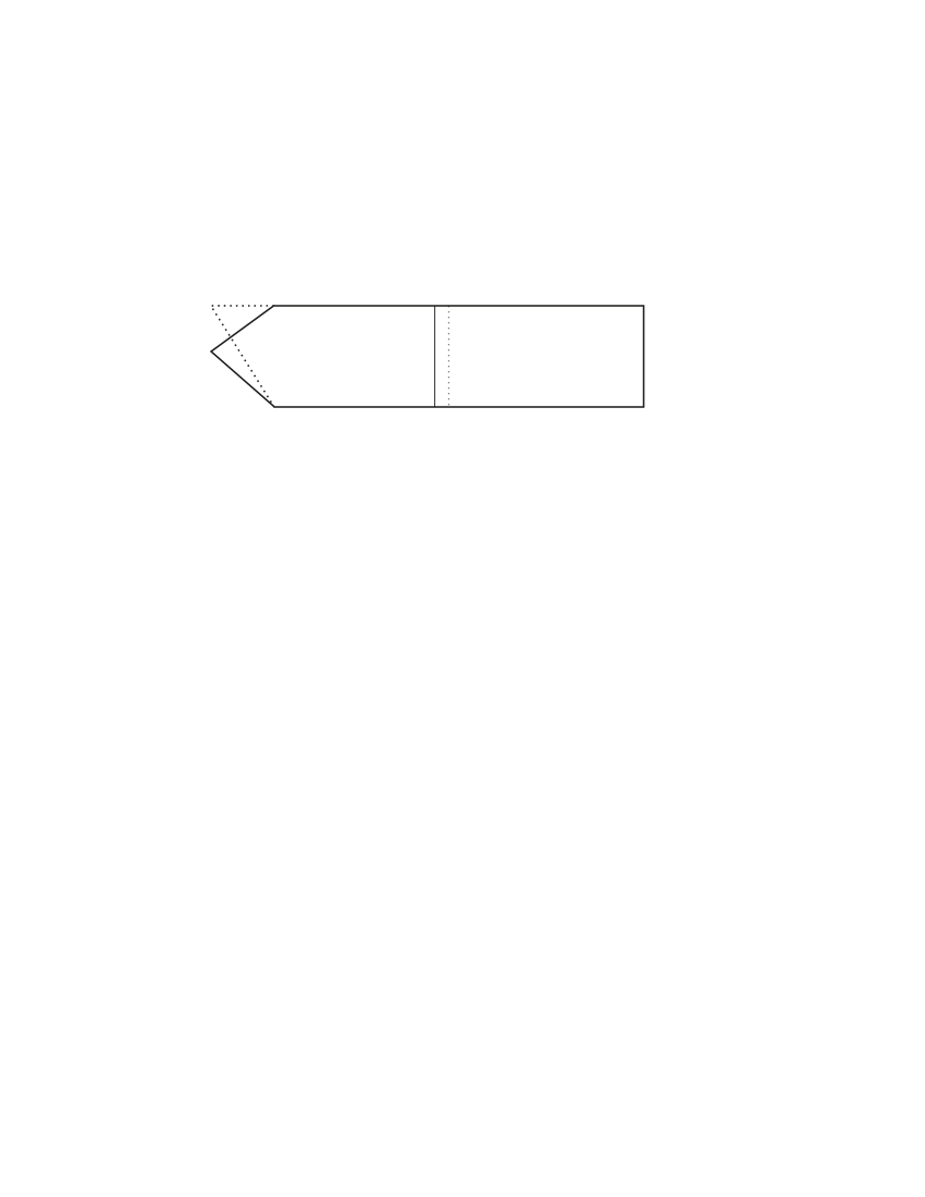
Figure 2. Two domains with same height function but distinct location of the nodal line.

Since $\phi_{0}$ is the symmetric decreasing rearrangement of $\tilde{\phi}_{0}$ around the point $1/2$, and since $(\sin\pi y)^{2}$ is symmetric decreasing itself, we have $\int_{0}^{1}\phi_{0}(y)(\sin\pi y)^{2}\,dy>\int_{0}^{1}\tilde{\phi}_{0}(y)(\sin\pi y)^{2}\,dy$, so Theorem 2 implies $a(\epsilon\phi_{0})\not=a(\epsilon\tilde{\phi}_{0})$ for some sufficiently small $\epsilon>0$. Since the domains associated with $\phi=\epsilon\phi_{0}$ and $\tilde{\phi}=\epsilon\tilde{\phi}_{0}$ clearly have the same height function, the theorem is proved.

References

- [1] Pavel Exner and Olaf Post, Convergence of spectra of graph-like thin manifolds., J. Geom. Phys. 54 (2005), no. 1, 77–115 (English).
- [2] P. Freitas and Krejčiřík, Location of the nodal set for thin curved tubes, To appear in Indiana Univ. Math. J.
- [3] Daniel Grieser, Spectra of graph neighborhoods and scattering, Preprint arXiv:0710.3405, 2007.
- [4] Daniel Grieser and David Jerison, Asymptotics of the first nodal line of a convex domain, Invent. Math. 125 (1996), no. 2, 197–219 (English).
- [5] by same author, The size of the first eigenfunction of a convex planar domain, J. Am. Math. Soc. 11 (1998), no. 1, 41–72 (English).
- [6] L. Guillopé, Théorie spectrale de quelques variétés à bouts, Ann.Sci.Éc.Norm.Supér. 22 (1989), no. 1, 137–160.
- [7] Andrew Hassell, Rafe Mazzeo, and Richard B. Melrose, Analytic surgery and the accumulation of eigenvalues, Commun. Anal. Geom. 3 (1995), no. 1, 115–222 (English).
- [8] David Jerison, The diameter of the first nodal line of a convex domain, Ann. Math., II. Ser. 141 (1995), no. 1, 1–33 (English).
- [9] Peter Kuchment and Hongbiao Zeng, Convergence of spectra of mesoscopic systems collapsing onto a graph., J. Math. Anal. Appl. 258 (2001), no. 2, 671–700.
- [10] S. Molchanov and B. Vainberg, Laplace operator in thin networks of thin fibers: Spectrum near the threshold, Preprint, arXiv:0704.2795, 2007.
- [11] Werner Müller, Eta invariants and manifolds with boundary., J. Differ. Geom. 40 (1994), no. 2, 311–377 (English).
- [12] Jinsung Park and Krzysztof P. Wojciechowski, Scattering theory and adiabatic decomposition of the -determinant of the Dirac Laplacian., Math. Res. Lett. 9 (2002), no. 1, 17–25 (English).
- [13] Jacob Rubinstein and Michelle Schatzman, Variational problems on multiply connected thin strips. I: Basic estimates and convergence of the Laplacian spectrum., Arch. Ration. Mech. Anal. 160 (2001), no. 4, 271–308.