Luminosity Dependence of the Quasar Clustering from SDSS DR5

Abstract

43024 objects, which were primarily identified as quasars in SDSS DR5 and have spectroscopic redshifts were used to study the luminosity dependence of the quasar clustering with the help of two different techniques. The obtained results reveal that brighter quasars are more clustered, but this dependence is weak, which is in agreement with the results by Porciani & Norberg [1] and theoretical predictions by Lidz et al. [2].

Key words: quasars, large-scale structure, clustering, luminosity.

PACS numbers: 98.65.Aj, 98.54.-h, 98.62.Ve.

Kyiv National Taras Shevchenko University, Glushkova ave., 2, 03127 Kyiv, Ukraine
hanna@univ.kiev.ua

1 Introduction

Determining the distribution of extragalactic objects is one of the most important problems of modern cosmology, because they are the only tracers of the dark matter, except anisotropy of the CMB, that helps us to realize the matter distribution on the redshifts of about 1000. Unfortunately even in the local Universe it is difficult to see the most faint galaxies, and when we go farther to larger redshifts, the most part of objects we can observe there with the modern ground-based telescopes used for large surveys are quasars as the most luminous objects. The matter distribution that we could reconstruct with the help of quasars is just like a light sketch, but it is all we have for today.

The quasars are nonuniform objects: they have various luminosities and are on the different stages of their evolution. Thus the reasonable question arises: how their clustering could depend on their physical properties, for example on their luminosity? According to different numerical simulations of galaxy mergers that incorporate black hole growth, this dependence has to exist because more luminous quasars are considered to be born in denser environment. In the main part of such models, in which the host halo mass correlates with the instantaneous luminosity of the quasars (see e.g. [3]), there should be a strong luminosity dependence of the quasar clustering. In the other type of such models, in which the host halo mass correlates with the peak luminosity of quasars, the luminosity dependence of the quasar clustering should be weaker because all of the quasars we see now, are considered to be similar objects but on different stages of their evolution (see [2] and references therein). It is worth to note, that the redshift distribution of the quasars is not the same for different luminosities due to possible evolution effects.

The largest quasar surveys are 2dF and SDSS. In contrast to 2dF, which is finished for today and has 2QZ catalogue as a result [4], SDSS [5] is in progress and the area covered by it is increasing. Only a part of objects primarily classified as quasars were justified by spectra analysis and were included into SDSS Quasar Catalogue IV [6]. However even photometric classification of quasars with color diagrams [7] is sufficient for using these objects for statistical purposes [8, 9].

Some attempts to find luminosity dependence of the quasar clustering have been made with different samples. E.g. Adelberg & Steidel [10], who worked with their own survey, pointed to luminosity independent quasar clustering. 2dF-team, that studied 2QZ survey and found the little redshift evolution in the amplitude of the power spectrum [11], [12] and significant increase in clustering amplitude at high redshifts [13, 14], detected only marginal evidence for quasars with brighter apparent magnitudes to have a stronger clustering amplitude [15]. Porciani and Norberg [1] also found weak luminosity dependence of the clustering in 2QZ survey. Furthermore they noted that samples with different redshifts show different trends in luminosity dependence: in the redshift bin $1.7<z<2.1$ the brightest quasars seem to be more clustered (have larger bias parameter); in the redshift bin $1.3<z<1.7$ the bias parameter seems to follow a U-shape; and the low redshift bin ($0.8<z<1.3$) does not show any particular trend. Myers et al. [8], working with $\sim$300,000 photometrically classified quasars from the 4th Data Release of the SDSS, detected no significant luminosity dependence and pointed out that a 3$\sigma$ detection of such effect requires a sample several times larger.

The present work deals with the study of the luminosity dependence of the quasar clustering for quasars from the Fifth Data Release of SDSS. The sample and its peculiarities are described in Section 2. The results of estimation of the correlation length as a function of luminosity are presented in Section 3. As we do not have such large sample, which we need, according to Myers et al. [8], for precise measurements of the correlation function, we used another technique, which is described in Section 4. Finally, Section 5 is dedicated to discussion of obtained results.

2 The Data

Table 1: The samples used for both methods. N is the number of objects for all given redshift interval ($z$). $M_{g,eff}$ is effective absolute magnitude, $N_{tot}$ is the number of objects with luminosity within given range ($M_{g}$) and $\bar{z}$ is the mean redshift.

$z$	$N$	$M_{g}$	$M_{g,eff}$	$N_{tot}$	$\bar{z}$
		$-24.5\div-23.5$	-24.1	2209	$0.937$
$0.80\div 1.10$	8621	$-25.5\div-24.5$	-25.0	4564	$0.965$
		$-26.5\div-25.5$	-25.9	1202	$0.984$
		$-25.0\div-24.0$	-24.6	2065	$1.213$
$1.10\div 1.35$	8619	$-26.0\div-25.0$	-25.5	5016	$1.230$
		$-27.0\div-26.0$	-26.3	1210	$1.244$
		$-25.5\div-24.5$	-25.1	2339	$1.466$
$1.35\div 1.59$	8579	$-26.5\div-25.5$	-25.9	4859	$1.480$
		$-27.5\div-26.5$	-26.8	1105	$1.490$
		$-25.5\div-24.5$	-25.2	1613	$1.702$
$1.59\div 1.83$	8511	$-26.5\div-25.5$	-26.1	4520	$1.704$
		$-27.5\div-26.5$	-26.9	2061	$1.719$
		$-26.0\div-25.0$	-25.6	2316	$1.968$
$1.83\div 2.20$	8694	$-27.0\div-26.0$	-26.5	4377	$1.977$
		$-28.0\div-27.0$	-27.3	1714	$2.019$

The sample of 43024 quasars with spectroscopic redshifts $0.8<z<2.2$ taken from the 5th Data Release (http://www.sdss.org/dr5/products/spectra/getspectra.html) of the Sloan Digital Sky Survey was uses to study the luminosity dependence of the quasar clustering. The calibrated apparent magnitudes in five SDSS photometric bands (u,g,r,i,z) are given not as a conventional Pogson astronomical magnitudes, but as asinh magnitudes [16]. Thus we firstly converted them to Pogson magnitudes. Then the absolute magnitudes in g-band ($M_{g}$) (the average wavelength $\lambda_{g}=4686^{\circ}$, magnitude limit $m_{g,lim}=22.2$) were calculated within the frame of $\Lambda$CDM-model with $\Omega_{tot}=1$ (spatially flat Universe), $\Omega_{M}=0.29$, $h=0.73$ [17].

The redshift distribution of quasars in the SDSS survey has several peaks and valleys, which could not be entirely explained by different selection effects, like similarity in colors of quasars within some redshift ranges or presence of some strong emission lines in different SDSS filter bands ([18] and references therein). But in spite of such peculiarities the whole distribution reveals a large hump on redshift of about 2 which agrees with an idea, according to which the most part of quasars had to be born at that time.

To study the luminosity dependence of the quasar clustering one should choose intervals of redshift small enough to avoid effects of redshift evolution (see e.g. [13], [14], [8], [9]). Therefore our sample was divided into 5 redshift intervals (see Table 1) with the similar number of quasars. The whole sample covers the so-called SDSS ’window’ (the redshift interval of SDSS data, where the photometrical selected quasars are the most uncontaminated due to specific character of the photometrical selection technique). Then in each redshift interval we selected 3 subsamples according to the absolute magnitude in g-band – ’bright’, ’medium’ and ’faint’ quasars. We chose absolute magnitude intervals of the same size ($\Delta M_{g}=1$).

3 Correlation functions

The first technique applied in this work to study the luminosity dependence of the quasar clustering is calculation of the redshift-space correlation function for objects with different luminosities. This means that the cross-correlation between quasars with luminosity within given range and quasars with any luminosity was calculated. Both in this case and in the second method, the measured distances are comoving distances in the reference frame of the local observer related to the first quasar. All the distances were measured within the frame of the $\Lambda$CDM-model and spatially flat Universe with the following parameters: $\Omega_{M}=0.29$ and $h=0.73$ [17].

According to [19] the probability to find a neighbour for i-th quasar in a spherical layer $[r,r+\Delta r]$ in the epoch $t$ is determined in terms of the two-point correlation function $\xi(r)$. Note, that all the calculations in this and the fourth sections were made in redshift-space, as we cannot separate cosmological redshift and peculiar velocities of quasars. Thus the total number of neighbours from the whole sample is

$$\Delta N(r)=4\pi\sum_{i}n(t_{i})\left[\frac{1}{3}[(r+\Delta r)^{3}-r^{3}]+\int_{r}^{r+\Delta r}\xi(\rho)\rho^{2}d\rho\right],$$

where $n(t_{i})$ is a mean number density of objects in the neighbourhood of i-th quasar. The similar estimation for random catalogue, which is considered to represent random spatial distribution of objects with no clustering, is

$$\Delta N^{\ast}(r)=\frac{4\pi}{3}\sum_{i}n^{\prime}(t_{i})[(r+\Delta r)^{3}-r^{3}].$$

Assuming

$$\sum_{i}n^{\prime}(t_{i})\approx\sum_{i}n(t_{i}),$$

we have

$$\frac{\Delta N(r)}{\Delta N^{\ast}(r)}-1=\frac{\int_{r}^{r+\Delta r}\xi(\rho)\rho^{2}d\rho}{\Delta r(r^{2}+r\Delta r+\Delta r^{2}/3)}.$$ (1)

The common power-low correlation function was used

$$\xi(r)=\left(\frac{r_{c}}{r}\right)^{\gamma},$$ (2)

thus the expression for fitting parameters $r_{c}$, $\gamma$ is the following

$$\frac{\Delta N(r)}{\Delta N^{\ast}(r)}-1=\frac{r_{c}^{\gamma}}{3-\gamma}\frac{(r+\Delta r)^{3-\gamma}-r^{3-\gamma}}{\Delta r(r^{2}+r\Delta r+\Delta r^{2}/3)}.$$ (3)

As the redshift-space correlation function has some distortions (like Finger of God effect and $\beta$-distortion) due to peculiar velocities of the objects (see e.g. [20, 21, 22]), and they differ on small and large scales, the correlation function of quasars cannot be approximated with one power-low function on all the scales. Thus the fitting was carried out within two intervals (2 Mpc $\div$ 10 Mpc and 10 Mpc $\div$ 50 Mpc) separately with $\Delta r=1$ Mpc.

For generation of the random catalogue the sky area covered by our sample was divided into $3^{\circ}\times 3^{\circ}$ parts and filled with the same number (43024 objects) of random points (random $\alpha$, $\delta$, $z$), preserving the number of objects in each part and the redshift distribution of initial catalogue. The absolute magnitudes of the objects ($M_{g}$) in random catalogue were taken from the initial one and permutated in random way, preserving redshift dependence of $M_{g}$. One hundred of such random samples were generated and $\Delta N^{\ast}(r)$ was calculated for each sample. Then the mean values $\langle\Delta N^{\ast}(r)\rangle_{100}$ were used instead of $\Delta N^{\ast}(r)$ for fitting with (3).

Table 2: Parameters of the redshift-space correlation function of quasars with different luminosities on scales 2 Mpc $\div$ 10 Mpc and 10 Mpc $\div$ 50 Mpc

$z$	$M_{g,eff}$	$\gamma$	$r_{c}$, $h^{-1}$Mpc	$\gamma$	$r_{c}$, $h^{-1}$Mpc
		($r\leq 10$ Mpc)	($r\leq 10$ Mpc)	($r\geq 10$ Mpc)	($r\geq 10$ Mpc)
	-24.1	$2.19\pm 0.30$	$6.20\pm 0.85$	$1.40\pm 0.32$	$7.37\pm 1.43$
$0.80\div 1.10$	-25.0	$2.05\pm 0.13$	$7.85\pm 0.57$	$1.56\pm 0.37$	$6.12\pm 1.73$
	-25.9	$1.85\pm 0.37$	$7.97\pm 1.18$	$2.04\pm 0.58$	$6.27\pm 1.94$
	-24.6	$1.66\pm 0.30$	$7.61\pm 2.21$	$1.18\pm 0.10$	$11.70\pm 1.21$
$1.12\div 1.35$	-25.5	$1.33\pm 0.19$	$8.31\pm 1.73$	$1.60\pm 0.28$	$7.95\pm 1.24$
	-26.3	$2.16\pm 0.24$	$7.24\pm 1.27$	$1.41\pm 0.33$	$6.91\pm 1.23$
	-25.1	$1.46\pm 0.17$	$8.17\pm 1.32$	$1.26\pm 0.17$	$10.21\pm 1.15$
$1.35\div 1.59$	-25.9	$1.83\pm 0.35$	$6.65\pm 1.28$	$1.87\pm 0.31$	$8.27\pm 1.17$
	-26.8	$1.65\pm 0.10$	$12.08\pm 1.34$	$2.30\pm 0.36$	$11.04\pm 0.97$
	-25.2	$1.51\pm 0.42$	$7.98\pm 1.86$	$1.43\pm 0.26$	$10.17\pm 1.96$
$1.59\div 1.83$	-26.1	$1.91\pm 0.21$	$7.72\pm 0.79$	$1.17\pm 0.11$	$7.75\pm 0.91$
	-26.9	$2.36\pm 0.52$	$6.44\pm 0.85$	$1.94\pm 0.52$	$4.43\pm 1.76$
	-25.6	$1.30\pm 0.19$	$11.93\pm 3.01$	$1.33\pm 0.23$	$12.06\pm 1.74$
$1.83\div 2.20$	-26.5	$2.34\pm 0.39$	$4.63\pm 0.88$	$1.40\pm 0.30$	$7.94\pm 1.51$
	-27.3	$1.34\pm 0.22$	$13.56\pm 4.51$	$2.27\pm 0.50$	$8.21\pm 2.08$

Here the errors were calculated in the following way. We obtain the ’initial’ values of the parameters ($r_{0}$, $\gamma$), find the deviations of experimental data from the theoretical one, construct random new ’experimental’ data using normal distribution and treating the theoretical values as mean values and obtained deviations as dispersions. We generated 100 of such sets of ’experimental’ data, found the parameters for each set, and then find the mean values of these parameters and their rms, which are presented in the Table 2.

As one can see, we cannot speak about any significant trend from these results. Some variations of the both parameters are present. E.g. for second and forth z intervals on the scales $r>10$ Mpc the correlation length is smaller for brighter quasars. On all the scales for third and fifth z intervals luminosity dependence of the correlation length seems to follow U-shape, which was found by Porciani & Norberg [1]. But all these differences along with variations of $\gamma$ are significant only on 1$\sigma$ level. Thus for varification of these results another another technique, which does not require very big samples was proposed in the next section.

4 A part of close pairs for quasars with different luminosities

The second method lies in direct estimation of a part of quasars with given luminosity which reside in environment with larger quasar density. For the initial sample S1 consider a subsample S2 of quasars having the absolute magnitude $M_{g}$ from a given interval $[M_{g,min},M_{g,max}]$. The number of quasars in subsample S2 is equal to $N_{tot}(M_{g,min}<M_{g}<M_{g,max})$. For any quasar from S2 we are looking for the nearest neighbours from S1 with any $M_{g}$ at the distance less than r. Let $N(r_{NN}<r,M_{g,min}<M_{g}<M_{g,max})$ be a number of quasars from S2 with $[M_{g,min},M_{g,max}]$ having the distance to the nearest neighbour from S2 less then r. Consider the following function

$$f(r,M_{g})=\frac{N(r_{NN}<r,M_{g,min}<M_{g}<M_{g,max})}{N_{tot}(M_{g,min}<M_{g}<M_{g,max})}.$$ (4)

If we fix the value of r, this function is an estimate of the portion of quasars with given luminosity, having the nearest neighbour distance less r, that could be an estimate of the portion of quasars with given luminosity reside in denser environment. Generally speaking, close pairs of quasars would not necessary reside in clusters. And the same function for the fifth nearest neighbour could be better estimate, but the sample is not large enough for this.

In our case initial samples (S1) are our five samples of quasars from different redshift intervals. In Table 1 $N$ is a number of objects in S1, $N_{tot}$ is a number of objects in subsamples S2.

Note that the function $f(r)$ is a complement to $g(r)$ introduced by White in [23] as

$$g(r)=\frac{N(r_{NN}>r)}{N_{tot}}.$$

It is readily seen that $f(r)=1-g(r)$. The function $g(r)$ is an estimate of the probability that the volume of radius r is empty. This is a complementary statistic to the correlation functions, because it depends on the correlation functions of all orders in an entirely symmetric way [23].

If there was no luminosity dependence of the quasar clustering, this function would not depend on absolute magnitude at all. For verification of this statement 100 artificial samples were generated for each from 5 samples in the following way: the absolute magnitudes in the catalogue were permutated in random way, preserving right ascensions, declinations and redshifts on their places. This means that the spatial distribution of quasars (clustering) remains the same, but any luminosity dependence has to disappear.

Results are shown in the Fig.1-5, where only curves for bright and faint quasars are shown for clearness. Open circles denote faint quasars, filled - bright ones. The same curves for permutated samples coincide, thus they are denoted with one curve with open triangles (only in the right parts of the plots). Note, that the errors shown on the plots are statistical ones for initial samples and rms for artificial samples. On the scales less than the clustering scales one can see that the curves for bright quasars lie higher than for faint ones. But the difference between the values $f(r)$ for quasars with different luminosities is statistically insignificant. Only for $1.35<z<1.59$ and $1.59<z<1.83$ this difference is more then 1$\sigma$ on scales of about $r_{c}$. Then the curves intersect on the scales of about half mean nearest neighbour distance. On larger scales the curves for faint quasars lie higher. And on the scale which could be some characteristic scale of the large-scale structure of the Universe these curves coincide. This scale increases with the redshift.

5 Discussion

As we can see from the Table 2 to obtain any reliable results with the first method one need much larger samples, which are unavailable for today. Moreover the correlation length is the spatial scale of clustering on the one hand and a measure of the clustering amplitude on the other hand. Thus it is not easy to interpret the first technique results unambiguously. That is why the second method seems to be better for this purpose because it is more direct and does not require such large samples.

From the results of the second method we can say that brighter quasars reside in closer pairs than faint ones. Note, that such splitting of f(r) curves on larges scales could also be the consequence of the different redshift distributions of the quasars with different luminosities. But we know, that the bright quasars represent higher redshifts and the quasar density decreases with the redshift, thus the inverse effect would be present. Anyway the difference between the mean redshift for subsamples of quasars with different luminosities (see the last column of Table 1) within each redshift interval is negligibly small and cannot affect the results.

Anyway this problem requires further investigations and improvement of the methods. It would be interesting to compare for example, the same $f(r)$ function for the fifth nearest neighbour or cross-correlation with galaxies. The last possibility could increase the sample, but this could be applied only for the lower redshift intervals, than those used in the present work.

Summing up the obtained results one can speal about luminosity dependence of the quasar clustering, but this dependence is not strong, which is in agreement with the results by Porciani & Norberg [1] and theoretical predictions by Lidz et al. [2]. But even if this dependence is weak, we do not have to neglect it. Note that when we estimate e.g. the correlation length of the quasars on the low redshift we obtain the mean correlation length averaged over all the quasars with different luminosities. But on the high redshifts the obtained results correspond only to the correlation length for bright quasars and do not reflect the whole picture. That is why possible effects of luminosity dependence of quasar clustering should be taken into account when studying the redshift evolution of it. But even so one should keep in mind that the quasars (as another AGNs) do not reflect the whole distribution of extragalactic objects because quasars are considered to reside in the strongest peaks of the matter density. This fact could explain larger values of the correlation function for quasars than for galaxies (see [24], [25] for comparision).

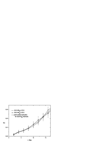
Figure 1: $f(r)$ for $0.80<z<1.10$. Left: for all scales. Right: for small scales.

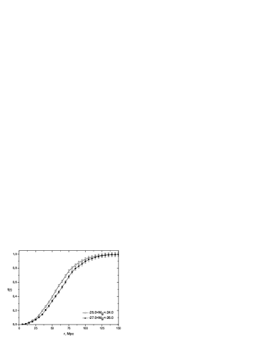
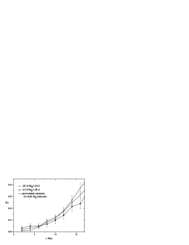
Figure 2: $f(r)$ for $1.10<z<1.35$. Left: for all scales. Right: for small scales.

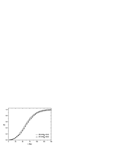
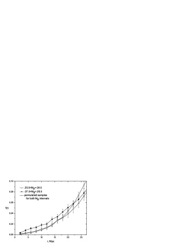
Figure 3: $f(r)$ for $1.35<z<1.59$. Left: for all scales. Right: for small scales.

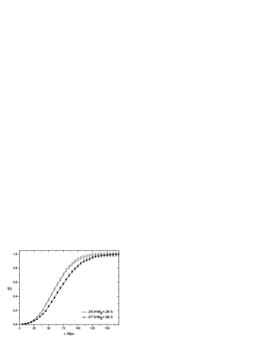
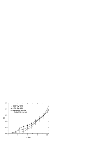
Figure 4: $f(r)$ for $1.59<z<1.83$. Left: for all scales. Right: for small scales.

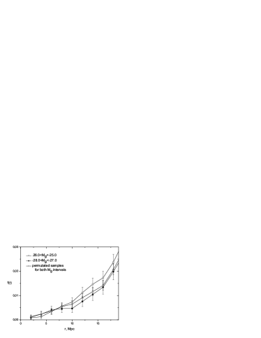
Figure 5: $f(r)$ for $1.83<z<2.20$. Left: for all scales. Right: for small scales.

References

- [1] C. Porciani, P. Norberg, Mon. Notic. Roy. Astron. Soc. 371, 4, 1824 (2006).
- [2] A. Lidz, P.F. Hopkins, Cox T.J., et al., Astrophys J. 641, 1, 41 (2006).
- [3] G. Kauffmann, M. Haehnelt, Mon. Notic. Roy. Astron. Soc. 311, 3, 576 (2000).
- [4] S.M. Croom, R.J. Smith, B.J. Boyle, et al., Mon. Notic. Roy. Astron. Soc., 349, 1397 (2004).
- [5] J.K. Adelman-McCarthy, M.A. Agüeros, S.S. Allam, et al., Astrophys. J. Supplements, in press (2007).
- [6] D.P. Schneider, P.B. Hall, G.T. Richards. 134, 1, 102 (2007).
- [7] G.T. Richards, R.C. Nichol, A.G. Gray, et al., Astrophys. J. Supplement Series. 155, 2, 257 (2004).
- [8] A.D. Myers, R.J. Brunner, R.C. Nichol, et al., Astrophys. J. 658, 1, 85 (2007).
- [9] A.D. Myers, R.J. Brunner, G.T. Richards, et al., Astropys. J. 638, 2, 622 (2006).
- [10] C.L. Adelberg, C.C. Steidel, Astrophys. J. 630, 2, 50 (2005).
- [11] F. Hoyle, P.J. Outram, T. Shanks, et al., Mon. Notic. Roy. Astron. Soc. 329, 2, 336 (2002).
- [12] P.J. Outram, F. Hoyle, T. Shanks, et al., Mon. Notic. Roy. Astron. Soc. 342, 2, 483 (2003).
- [13] S.M. Croom, B.J. Boyle, T. Shanks, et al., Mon. Notic. Roy. Astron. Soc. 356, 2, 415 (2005).
- [14] S.M. Croom, T. Shanks, B.J. Boyle, et al., Mon. Notic. Roy. Astron. Soc. 325, 2, 483 (2001).
- [15] S.M. Croom, B.J. Boyle, N.S. Loaring, et al., Mon. Notic. Roy. Astron. Soc. 335, 2, 459 (2002).
- [16] R.H. Lupton, J.E. Gunn, A.S. Szalay, Astron. J. 118, 1406 (1999).
- [17] D.N. Spergel, R. Bean, O. Dor, et al., Astrophys. J. Supplement Series 170, 2, 377 (2007).
- [18] M.B. Bell, D. McDiarmid, Astrophys. J. 648, 1, 140 (2006).
- [19] P.J.E. Peebles, The Large-Scale Structure of the Universe (Princeton University Press, 1980).
- [20] T. Matsubara, Ya. Suto, Astrophys. J. Letters, 470, L1 (1996).
- [21] W.E. Ballinger, J.A. Peacock, A.F. Heavens, Mon. Notic. Roy. Astron. Soc., 282, 877 (1996).
- [22] J.A. Peacock, S.J. Dodds, Mon. Notic. Roy. Astron. Soc., 267, 1020 (1994).
- [23] S.D.M. White, Mon. Not. Roy. Astron. Soc. 186, 145 (1979).
- [24] C. Blake, T. Mauch, E.M. Sadler, Mon. Notic. Roy. Astron. Soc. 347, 3, 787 (2004).
- [25] E.A. Gonzalez-Solares, S. Oliver, C. Gruppioni, et al., Mon. Notic. Roy. Astron. Soc. 352, 1, 44 (2004).