Hydrodynamic stability and mode coupling in Keplerian flows: local strato-rotational analysis

Abstract

Aims. We present a qualitative analysis of key (but yet unappreciated) linear phenomena in stratified hydrodynamic Keplerian flows: (i) the occurrence of a vortex mode, as a consequence of strato-rotational balance, with its transient dynamics; (ii) the generation of spiral-density waves (also called inertia-gravity or $g\Omega$ waves) by the vortex mode through linear mode coupling in shear flows.

Methods. Non-modal analysis of linearized Boussinesq equations were written in the shearing sheet approximation of accretion disk flows.

Results. It is shown that the combined action of rotation and stratification introduces a new degree of freedom, vortex mode perturbation, which is in turn linearly coupled with the spiral-density waves. These two modes are jointly able to extract energy from the background flow, and they govern the disk dynamics in the small-scale range. The transient behavior of these modes is determined by the non-normality of the Keplerian shear flow. Tightly leading vortex mode perturbations undergo substantial transient growth, then, becoming trailing, inevitably generate trailing spiral-density waves by linear mode coupling. This course of events – transient growth plus coupling – is particularly pronounced for perturbation harmonics with comparable azimuthal and vertical scales, and it renders the energy dynamics similar to the 3D unbounded plane Couette flow case.

Conclusions. Our investigation strongly suggests that the so-called bypass concept of turbulence, which has been recently developed by the hydrodynamic community for spectrally stable shear flows, can also be applied to Keplerian disks. This conjecture may be confirmed by appropriate numerical simulations that take the vertical stratification and consequent mode coupling into account in the high Reynolds number regime.

1 Introduction

According to classical fluid dynamics, unmagnetized disk flows in Keplerian rotation (more generally: with angular momentum increasing outward and with no extremum of vorticity) are spectrally stable; however, there is irrefutable observational evidence that such disks have to be turbulent. Due to this apparent contradiction, disk turbulence is often considered as some sort of mystery. However, an analogous dilemma that existed in laboratory/engineering flows has been solved by the hydrodynamic community in the 90s of the last century, where a breakthrough was accomplished in the comprehension of turbulence in spectrally/asymptotically stable shear flows (e.g. in the plane Couette flow).

Let us briefly recall the essence of that breakthrough (see Chagelishvili et al. 2003 for details). Traditional stability theory followed the approach of Rayleigh (1880) where the instability is determined by the presence of exponentially growing modes that are solutions of the linearized dynamic equations. Only recently has one become aware that operators involved in the the modal analysis of plane shear flows are not normal, hence that the corresponding eigenfunctions are non-orthogonal and would strongly interfere (Reddy et al. 1993). For this reason, the emphasis was shifted in the 90s from the analysis of long time asymptotic flow stability to the study of short time behavior. It was established that asymptotically/Rayleigh stable flows allow for linear transient growth of vortex and/or wave mode perturbations (cf. Gustavsson 1991; Butler and Farrell 1992; Reddy and Henningson 1993; Trefethen et al. 1993). This fact incited a number of fluid dynamicists to examine the possibility of a subcritical transition to turbulence, with the linear stable flow finding a way to bypass the usual route to turbulence (via linear classical/exponential instability). On closer examination, the perturbations reveal rich and complex behavior in the early transient phase, which leads to the expectation that they may become self-sustaining when there is nonlinear positive feedback.

Based on the interplay of linear transient growth and nonlinear positive feedback, a new concept emerged in the hydrodynamic community for the onset of turbulence in spectrally stable shear flows and was named bypass transition (cf. Boberg & Brosa 1988; Butler & Farrell 1992; Farrell & Ioannou 1993; Reddy & Henningson 1993; Gebhardt & Grossmann 1994; Henningson & Reddy 1994; Baggett et al. 1995; Grossmann 2000; Reshotko 2001; Chagelishvili et al. 2002; Chapman 2002). The bypass scenario differs fundamentally from the classical scenario of turbulence. In the classical model, exponentially growing perturbations permanently supply energy to the turbulence and they do not need any nonlinear feedback for their self-sustenance, so the role of nonlinear interaction is just to reduce the scale of perturbations to that of viscous dissipation. In the bypass model, nonlinearity plays a key role. The nonlinear processes are conservative, but in the case of positive feedback, they ensure the repopulation of perturbations that are able to extract energy transiently from the mean flow. The self-sustenance of turbulence is then the result of a subtle and balanced interplay of linear transient growth and nonlinear positive feedback. Consequently, thorough examination of the nonlinear interaction between perturbations is a problem of primary importance, and the first step is to search and to describe the linear perturbation modes that will participate in the nonlinear interactions.

Such linear transient growth is also at work in rotating hydrodynamic disk flows; however, the Coriolis force causes a quantitative reduction of the growth rate there which delays the onset of turbulence. Keplerian flows are therefore expected to become turbulent for Reynolds numbers a few order of magnitudes higher than for plane subcritical flows (see: Longaretti 2002; Tevzadze et al. 2003). The possibility of an alternate route to turbulence gave new impetus to the research on the dynamics of astrophysical disks (Lominadze et al. 1988; Richard & Zahn 1999; Richard 2001; Ioannou & Kakouris 2001; Tagger 2001; Longaretti 2002; Chagelishvili et al. 2003; Tevzadze et al. 2003; Klahr & Bodenheimer 2003; Yecko 2004; Afshordi et al. 2004 Umurhan & Regev 2004; Umurhan & Shaviv 2005; Klahr 2004; Bodo et al. 2005; Mukhopadhyay et al. 2005; Barraco & Marcus 2005; Johnson & Gammie 2005a, 2005b; Umurhan 2006). By adapting the progress of the hydrodynamic community to the disks flow, this research is promising for solving the disks’ hydrodynamic turbulence problem.

But it remains to be seen whether this route to turbulence actually applies to astrophysical disks. Compared to plane shear flows, these possess two additional properties: differential rotation and vertical stratification. Separate studies of these factors show that each exerts a stabilizing effect on the flow: these include numerical calculation of the stability of unstratified flows by Shen et al. (2006), experiments on Keplerian rotation without stratification by Ji et al. (2006), estimates of the growth rates with stratification by Brandenburg & Dintrans (2006). However, it appears that the combined action of differential rotation and stratification introduces a new degree of freedom that may influence the flow stability and lead to turbulence at a high enough Reynolds number. Indeed, it has been shown that strato-rotational flows may exhibit global instability in bounded domains (Dubrulle et al. 2005). However, it is probable that local disk dynamics will also lead to hydrodynamic turbulence. The study of the linear perturbations in strato-rotational flow in the local limit can be found in Tevzadze et al. (2003; hereafter T03); it is shown there that the combined action of rotation and stratification generates an aperiodic vortex mode, which undergoes nonmodal transient growth. We conjecture that this transient growth may be the main energy source for the turbulence in the bypass scenario.

Although the importance of the transient exchange of energy between perturbations and mean flow has now been realized by most working in the field, only a few seem aware that another linear process may play also a crucial role, namely the linear coupling of modes, which allows for transient exchange of energy between them. As shown by Chagelishvili et al. (1997a,b) and Gogoberidze et al. (2004), the energy exchange between modes is inherent to shear flows (as the transient exchange of energy between the mean flow and perturbations), and it determines in many respects the diversity of perturbation modes and, therefore, of nonlinear processes. Once one fully realizes the role of nonlinear processes in the bypass concept discussed above, it becomes evident that the neglect of linear mode coupling may lead to an incorrect picture of nonlinear (and, consequently, turbulent) phenomena.

There are signs of such linear mode coupling in the simulations performed by Klahr (2004), Barraco & Marcus (2005), and Brandenburg & Dintrans (2006), but apparently they were not identified as such. Compressive waves are present in the simulation by Johnson & Gammie (2005b), along with vortical perturbations, but their origin is not recognized, namely linear mode coupling. On this mode coupling, attention is focused in T03 and Bodo et al. (2005). The latter paper studies the linear dynamics of an imposed two-dimensional pure vortex mode perturbation, in a compressible Keplerian disk with constant mean pressure and density. (Two-dimensionality, i.e. the neglect of cross-disk variation, is only correct for perturbations with characteristic scales close to or larger than the vertical stratification scale of the disk.) Two modes – a vortex mode and a spiral-density wave mode – exist in the system, and they are strongly coupled. This investigation points out the importance of mode coupling and the necessity of considering compressibility for dynamic processes with characteristic scales close to or larger than the disk thickness.

In T03 we studied the linear dynamics of three-dimensional small-scale perturbations (with characteristic length scales much shorter than the disk thickness) in compressible, vertically (stably) stratified Keplerian disks. The first novelty presented in that paper is the occurrence of an interplay between the disk rotation and stratification. Separately, each of these factors is stabilizing. However, their interplay gives rise to a new vortex/aperiodic mode that is able to extract the basic flow energy transiently. The second novelty is the existence of a linear coupling of that vortex mode with spiral-density wave (SDW) modes, that makes SDWs valuable participants of the dynamical processes. Furthermore, we compared the linear dynamics of the small-scale perturbations in steady stratified disks with that of the perturbations in unbounded plane Couette flow. We showed that just the linear coupling of the disk modes makes the dynamics in the disk and plane flows similar to each other (provided the Reynolds number of the disk flow is chosen about three orders of magnitudes higher than in the plane flow). This similarity suggests that the bypass concept can also be applied to disk flow and it further motivates investigation in this direction.

In this respect, the present paper is a sequel of T03: we focus again on the mathematical and physical aspects of mode coupling, while introducing a significant simplification by neglecting the rotational-acoustic waves. This is justified by the fact that the characteristic timescale of these modes is much shorter than for the two other modes, when the characteristic lengthscale of the perturbations is much shorter than the disk thickness. Then the rotational-acoustic waves are not coupled to the vortex and SDW modes, and they play a negligible role in the slow, small-scale dynamics. That is why we can cut out the rotational-acoustic waves (i.e., the flow compressibility) without detriment to the dynamic picture and confine ourselves to the Boussinesq approximation. Keeping just vortex and SDW modes, this approximation simplifies mathematical aspects of the problem and allows an advance in the analytical description and comprehension of mode coupling.

The paper is organized as follows. In Sect. 2 we introduce the physical approximations and the mathematical formalism, and describe the linear strato-rotational balance and the perturbation modes. In Sect. 3 we present the qualitative and quantitative analysis of the linear dynamics of perturbations. We summarize and discuss the results in Sect. 4.

2 Disk model

The dynamics of a rotating flow in a central gravity field is governed by the Navier Stokes equations, which are written here in the cylindrical coordinates:

$${\partial\rho\over\partial t}+{\partial\over\partial r}(\rho V_{r})+{1\over r}{\partial\over\partial\phi}(\rho V_{\phi})+{\partial\over\partial z}(\rho V_{z})=0,$$ (1)

$${\partial V_{r}\over\partial t}+({\bf V}\cdot\nabla)V_{r}-{V_{\phi}^{2}\over r}=-{1\over\rho}{\partial P\over\partial r}-{\partial\Phi\over\partial r},$$ (2)

$${\partial V_{\phi}\over\partial t}+({\bf V}\cdot\nabla)V_{\phi}+{V_{r}V_{\phi}\over r}=-{1\over\rho r}{\partial P\over\partial\phi},$$ (3)

$${\partial V_{z}\over\partial t}+({\bf V}\cdot\nabla)V_{z}=-{1\over\rho}{\partial P\over\partial z}-{\partial\Phi\over\partial z},$$ (4)

$$\rho=\rho(P,S),$$ (5)

where

$$({\bf V}\cdot\nabla)\equiv V_{r}{\partial\over\partial r}+{V_{\phi}\over r}{\partial\over\partial\phi}+V_{z}{\partial\over\partial z}$$ (6)

is the component in convective derivative in cylindrical coordinate system. For the equilibrium state we choose the thin disk approximation with ${\bf V_{0}}=(0,V_{0\phi},0)$, with ${\bf\Omega}=(0,0,\Omega({\bf r}))$ and $V_{0\phi}=r\Omega({\bf r})$. Hence, we neglect self gravity and assume that the disk is rotationally supported. Vertical gravity acceleration and stratification scaleheight can be defined as follows:

$${\partial\Phi({\bf r})\over\partial z}=\Omega^{2}({\bf r})z\approx{\rm sgn}(z)g$$ (7)

$${1\over P_{0}(z)}{\partial P_{0}(z)\over\partial z}={1\over\rho_{0}(z)}{\partial\rho_{0}(z)\over\partial z}\equiv-k_{H}.$$ (8)

We consider isothermal equilibrium and study small-scale perturbations employing local approximation for further analysis.

2.1 The shearing sheet formalism in the Boussinesq approximation

For the purpose of the linear analysis, we employ local co-rotating shearing sheet:

$$x\equiv r-r_{0},\leavevmode\nobreak\ \leavevmode\nobreak\ \leavevmode\nobreak\ \leavevmode\nobreak\ \leavevmode\nobreak\ y\equiv r_{0}(\phi-\Omega_{0}t),\leavevmode\nobreak\ \leavevmode\nobreak\ \leavevmode\nobreak\ \leavevmode\nobreak\ \leavevmode\nobreak\ z=z\leavevmode\nobreak\ .$$ (9)

$${x\over r_{0}},{y\over r_{0}},{z\over r_{0}}\ll 1,$$ (10)

where we neglect the effect of global flow curvature and study the local influence of the differential rotation on the perturbations (see Goldreich & Linden-Bell 1965). We introduce the linear perturbations as follows:

$${\bf V}={\bf V}_{0}+{\bf V}^{\prime},\leavevmode\nobreak\ \leavevmode\nobreak\ \leavevmode\nobreak\ P=P_{0}+P^{\prime},\leavevmode\nobreak\ \leavevmode\nobreak\ \leavevmode\nobreak\ \rho=\rho_{0}+\rho^{\prime}\leavevmode\nobreak\ .$$ (11)

For further simplification we employ the Boussinesq approximation to neglect compressibility effects. We assume that $k_{H}={\rm const}$ and restrict analysis to the perturbations with shorter lengthscales than the vertical stratification scale of the disk flow. Hence, the system of equations that governs the perturbation dynamics in the considered limit reduces to

$$\left({\partial\over\partial t}+2Ax{\partial\over\partial y}\right)V_{x}^{\prime}-2\Omega_{0}V_{y}^{\prime}+{1\over\rho_{0}}{\partial P^{\prime}\over\partial x}=0,$$ (12)

$$\left({\partial\over\partial t}+2Ax{\partial\over\partial y}\right)V_{y}^{\prime}+2(\Omega_{0}+A)V_{x}^{\prime}+{1\over\rho_{0}}{\partial P^{\prime}\over\partial y}=0,$$ (13)

$$\left({\partial\over\partial t}+2Ax{\partial\over\partial y}\right)V_{z}^{\prime}+{1\over\rho_{0}}{\partial P^{\prime}\over\partial z}+g{\rho^{\prime}\over\rho_{0}}=0,$$ (14)

$$\left({\partial\over\partial t}+2Ax{\partial\over\partial y}\right){\rho^{\prime}\over\rho_{0}}-k_{H}V_{z}^{\prime}=0,$$ (15)

$${\partial V_{x}^{\prime}\over\partial x}+{\partial V_{y}^{\prime}\over\partial y}+{\partial V_{z}^{\prime}\over\partial z}=0.$$ (16)

Here for brevity $\rho_{0}\equiv\rho_{0}(0)$, and only the $z>0$ case is considered. We use standard Oort’s constants to quantify the radial velocity shear:

$$A\equiv{1\over 2}\left[r{\partial\Omega\over\partial r}\right]_{r=r_{0}}\!\!\!\!\!=-{3\over 4}\Omega_{0},\leavevmode\nobreak\ \leavevmode\nobreak\ \leavevmode\nobreak\ {\rm and}\leavevmode\nobreak\ \leavevmode\nobreak\ \leavevmode\nobreak\ A+B=-\Omega_{0}.$$ (17)

Following the standard procedure of nonmodal analysis, we employ spatial Fourier expansion of perturbations with specific phase variation:

$$\left\{\begin{array}[]{c}P^{\prime}({\bf r},t)\\ \rho^{\prime}({\bf r},t)\\ {\bf V}^{\prime}({\bf r},t)\end{array}\right\}=\left\{\begin{array}[]{c}p({\bf k},t)\\ \varrho({\bf k},t)\\ {\bf v}({\bf k},t)\end{array}\right\}\exp({\rm i}k_{x}(t)x+{\rm i}k_{y}y+{\rm i}k_{z}z),$$ (18)

where

$$k_{x}(t)=k_{x}(0)-2Ak_{y}t\leavevmode\nobreak\ .$$ (19)

This leads to the linear system of ODE that governs the dynamics of SFH in the considered flow:

$${{\rm d}\over{\rm d}t}v_{x}(t)=2\Omega_{0}v_{y}(t)-{\rm i}k_{x}(t){p(t)\over\rho_{0}},$$ (20)

$${{\rm d}\over{\rm d}t}v_{y}(t)=2Bv_{x}(t)-{\rm i}k_{y}{p(t)\over\rho_{0}},$$ (21)

$${{\rm d}\over{\rm d}t}v_{z}(t)=-{\rm i}k_{z}{p(t)\over\rho_{0}}-g{\varrho(t)\over\rho_{0}},$$ (22)

$${{\rm d}\over{\rm d}t}{\varrho(t)\over\rho_{0}}=k_{H}v_{z}(t),$$ (23)

$$k_{x}(t)v_{x}(t)+k_{y}v_{y}+k_{z}v_{z}=0.$$ (24)

Introducing new notations for pressure and density

$$P\equiv{{\rm i}p\over\rho_{0}}\leavevmode\nobreak\ ,\leavevmode\nobreak\ \leavevmode\nobreak\ \leavevmode\nobreak\ D\equiv{\varrho\over\rho_{0}}\leavevmode\nobreak\ ,$$ (25)

we obtain an ODE system that does not explicitly contain complex coefficients. The system is characterized by a temporal invariant that corresponds to the linear perturbation of the potential vorticity:

$$W\equiv k_{x}(t)v_{y}-k_{y}v_{x}+2B{k_{z}\over k_{H}}D={\rm const.}$$ (26)

With straightforward simplifications

$$P=-g{k_{z}\over k^{2}}D+{2\Omega_{0}\over k^{2}}\left(k_{x}(t)v_{y}-k_{y}v_{x}\right)-4A{k_{y}\over k^{2}}v_{x}\leavevmode\nobreak\ ,$$ (27)

we reduce the governing equations to the following ODE system that is third order in time:

$${{\rm d}\over{\rm d}t}v_{x}(t)=\leavevmode\nobreak\ \leavevmode\nobreak\ \leavevmode\nobreak\ \leavevmode\nobreak\ \leavevmode\nobreak\ \leavevmode\nobreak\ \leavevmode\nobreak\ \leavevmode\nobreak\ \leavevmode\nobreak\ \leavevmode\nobreak\ \leavevmode\nobreak\ \leavevmode\nobreak\ \leavevmode\nobreak\ \leavevmode\nobreak\ \leavevmode\nobreak\ \leavevmode\nobreak\ \leavevmode\nobreak\ \leavevmode\nobreak\ \leavevmode\nobreak\ \leavevmode\nobreak\ \leavevmode\nobreak\ \leavevmode\nobreak\ \leavevmode\nobreak\ \leavevmode\nobreak\ \leavevmode\nobreak\ \leavevmode\nobreak\ \leavevmode\nobreak\ \leavevmode\nobreak\ \leavevmode\nobreak\ \leavevmode\nobreak\ \leavevmode\nobreak\ \leavevmode\nobreak\ \leavevmode\nobreak\ \leavevmode\nobreak\ \leavevmode\nobreak\ \leavevmode\nobreak\ \leavevmode\nobreak\ \leavevmode\nobreak\ \leavevmode\nobreak\ \leavevmode\nobreak\ \leavevmode\nobreak\ \leavevmode\nobreak\ \leavevmode\nobreak\ \leavevmode\nobreak\ \leavevmode\nobreak\ \leavevmode\nobreak\ \leavevmode\nobreak\ \leavevmode\nobreak\ \leavevmode\nobreak\ \leavevmode\nobreak\ \leavevmode\nobreak\ \leavevmode\nobreak\ \leavevmode\nobreak\ \leavevmode\nobreak\ \leavevmode\nobreak\ \leavevmode\nobreak\$$ (28)

$$=2(\Omega_{0}+2A){k_{x}(t)k_{y}\over k^{2}(t)}v_{x}+2\Omega_{0}{k_{y}^{2}+k_{z}^{2}\over k^{2}(t)}v_{y}+g{k_{x}(t)k_{z}\over k^{2}(t)}D\leavevmode\nobreak\ ,$$

$${{\rm d}\over{\rm d}t}v_{y}(t)=\leavevmode\nobreak\ \leavevmode\nobreak\ \leavevmode\nobreak\ \leavevmode\nobreak\ \leavevmode\nobreak\ \leavevmode\nobreak\ \leavevmode\nobreak\ \leavevmode\nobreak\ \leavevmode\nobreak\ \leavevmode\nobreak\ \leavevmode\nobreak\ \leavevmode\nobreak\ \leavevmode\nobreak\ \leavevmode\nobreak\ \leavevmode\nobreak\ \leavevmode\nobreak\ \leavevmode\nobreak\ \leavevmode\nobreak\ \leavevmode\nobreak\ \leavevmode\nobreak\ \leavevmode\nobreak\ \leavevmode\nobreak\ \leavevmode\nobreak\ \leavevmode\nobreak\ \leavevmode\nobreak\ \leavevmode\nobreak\ \leavevmode\nobreak\ \leavevmode\nobreak\ \leavevmode\nobreak\ \leavevmode\nobreak\ \leavevmode\nobreak\ \leavevmode\nobreak\ \leavevmode\nobreak\ \leavevmode\nobreak\ \leavevmode\nobreak\ \leavevmode\nobreak\ \leavevmode\nobreak\ \leavevmode\nobreak\ \leavevmode\nobreak\ \leavevmode\nobreak\ \leavevmode\nobreak\ \leavevmode\nobreak\ \leavevmode\nobreak\ \leavevmode\nobreak\ \leavevmode\nobreak\ \leavevmode\nobreak\ \leavevmode\nobreak\ \leavevmode\nobreak\ \leavevmode\nobreak\ \leavevmode\nobreak\ \leavevmode\nobreak\ \leavevmode\nobreak\ \leavevmode\nobreak\ \leavevmode\nobreak\ \leavevmode\nobreak\ \leavevmode\nobreak\$$ (29)

$$\left(2B{k_{x}^{2}(t)+k_{z}^{2}\over k^{2}(t)}+2A{k_{y}^{2}\over k^{2}(t)}\right)v_{x}-2\Omega_{0}{k_{x}(t)k_{y}\over k^{2}(t)}v_{y}+g{k_{y}k_{z}\over k^{2}(t)}D\leavevmode\nobreak\ ,$$

$${{\rm d}\over{\rm d}t}D(t)=-{k_{H}\over k_{z}}\left(k_{x}(t)v_{x}+k_{y}v_{y}\right)\leavevmode\nobreak\ ,$$ (30)

with

$$v_{z}(t)=-{1\over k_{z}}\left(k_{x}(t)v_{x}(t)+k_{y}v_{y}(t)\right)\leavevmode\nobreak\ .$$ (31)

These equations will be employed in the numerical calculations. The spectral energy of the perturbation SFH can be derived from the sum of thermal and thermobaric energies (see Eckart 1960), which in the considered Boussinesq approximation will read as

$$E_{k}(t)={\rho_{0}\over 2}\left(u_{x}^{2}(t)+u_{y}^{2}(t)+u_{z}^{2}(t)+{g\over k_{H}}D^{2}(t)\right)\leavevmode\nobreak\ .$$ (32)

2.2 Rigid rotation limit: strato-rotational balance and perturbation modes

In the shearless limit ($A=0$, $B=-\Omega$), the operators that intervene in the system above become normal, and it is easy to derive its dispersion relation. Its roots will help us to understand the mode behavior in the Keplerian flow, although the results are not applicable as such. Taking the Fourier expansion of the perturbations in time $\propto\exp({\rm i}\omega t)$, we obtain

$$\omega\left(\omega^{2}-4\Omega_{0}^{2}{k_{z}^{2}\over k^{2}}-N^{2}{k_{\perp}^{2}\over k^{2}}\right)=0\leavevmode\nobreak\ ,$$ (33)

where

$$N^{2}\equiv gk_{H}=-{g\over\rho_{0}(z)}{\partial\rho_{0}(z)\over\partial z}$$ (34)

is the Brunt-Väisälä frequency that is constant in our formalism. The solutions to this dispersion equation consist of two modes that are generally decoupled in the zero shear limit:

i) A spiral-density wave (SDW) – or inertia-gravity wave – that describes the oscillations due to the Coriolis force and to the vertical buoyancy;

ii) A stationary vortex mode with zero frequency. This stationary solution describes aperiodic perturbations to the vertical strato-rotational balance that can be directly derived from Eqs. (12-16):

$$2\Omega_{0}{\partial\over\partial z}{\rm curl}V^{\prime}=-g\left({\partial^{2}\over\partial x^{2}}+{\partial^{2}\over\partial y^{2}}\right)\rho^{\prime}\leavevmode\nobreak\ ,$$ (35)

where ${\rm curl}V^{\prime}$ is the vertical component of the vorticity:

$${\rm curl}V^{\prime}\equiv{\partial V_{y}^{\prime}\over\partial x}-{\partial V_{x}^{\prime}\over\partial y}\leavevmode\nobreak\ .$$ (36)

We see that stationary vorticity perturbations in the disk plane (lefthand side of the Eq. 35) can be sustained by density perturbations (righthand side of the Eq. 35), provided that both rotation ($\Omega_{0}$) and vertical stratification ($g$) are present. It is the stationary vortex mode, which appears due to the strato-rotational balance, that becomes dynamically active in the shear case (for $\leavevmode\nobreak\ A\not=0$) and is then able to extract the mean flow energy.

3 Qualitative analysis of the linear dynamics: transient growth and mode coupling

The numerical study of SFHs dynamics is governed by Eqs. (28-31). However, to clarify the physical nature of the perturbations and their linear dynamics, it is advisable to rewrite them in another form. Introducing a new variable

$$\Phi(t)\equiv{k(t)\over k_{\perp}(t)}D(t)\leavevmode\nobreak\ ,$$ (37)

from Eqs. (27),(29)-(31) one obtains the second-order inhomogeneous differential equation

$$\left\{{{\rm d^{2}}\over{\rm d}t^{2}}+\omega_{\phi}^{2}(t)\right\}\Phi(t)=f_{\phi}(t)W\leavevmode\nobreak\ ,$$ (38)

with the frequency

$$\omega_{\phi}^{2}(t)=N^{2}{k^{2}_{\perp}\over k^{2}}+4\Omega_{0}(\Omega_{0}+A){k^{2}_{z}\over k^{2}}+\leavevmode\nobreak\ \leavevmode\nobreak\ \leavevmode\nobreak\ \leavevmode\nobreak\ \leavevmode\nobreak\ \leavevmode\nobreak\ \leavevmode\nobreak\ \leavevmode\nobreak\ \leavevmode\nobreak\ \leavevmode\nobreak\ \leavevmode\nobreak\ \leavevmode\nobreak\ \leavevmode\nobreak\ \leavevmode\nobreak\ \leavevmode\nobreak\ \leavevmode\nobreak\ \leavevmode\nobreak\ \leavevmode\nobreak\ \leavevmode\nobreak\ \leavevmode\nobreak\ \leavevmode\nobreak\ \leavevmode\nobreak\ \leavevmode\nobreak\ \leavevmode\nobreak\ \leavevmode\nobreak\ \leavevmode\nobreak\ \leavevmode\nobreak\ \leavevmode\nobreak\$$ (39)

$$\leavevmode\nobreak\ \leavevmode\nobreak\ \leavevmode\nobreak\ \leavevmode\nobreak\ \leavevmode\nobreak\ \leavevmode\nobreak\ \leavevmode\nobreak\ \leavevmode\nobreak\ \leavevmode\nobreak\ \leavevmode\nobreak\ \leavevmode\nobreak\ \leavevmode\nobreak\ +\left(8A\Omega_{0}-4A^{2}{k^{2}_{x}\over k^{2}}+12A^{2}{k^{2}_{y}\over k^{2}_{\perp}}\right){k_{y}^{2}k_{z}^{2}\over k^{2}k_{\perp}^{2}}\leavevmode\nobreak\ ,$$

and the coupling function

$$f_{\phi}(t)=-2{k_{H}k_{z}\over{kk_{\perp}}}\left(\Omega_{0}+2A{k_{y}^{2}\over k_{\perp}^{2}}\right)\leavevmode\nobreak\ .$$ (40)

Equation (38) is essentially the same as the main dynamical equation of Chagelishvili et al. (1997), in which one form of mode linear coupling in shear flows has been described, namely the generation of wave SFHs by related SFHs of vortex mode perturbations. Thus one can borrow the qualitative analysis from that paper. As a result, Eq. (38) describes the dynamics of SFHs of two different modes of perturbations:
(a) the spiral-density wave mode (SDW), which is described by the general solution of the corresponding homogeneous equation. Consequently, this wave mode has zero potential vorticity (i.e. $W=0$, cf. Eq. 26). Note that the frequency $\omega_{\phi}(t)$ of the wave SFHs is time-dependent.
(b) the aperiodic vortex mode, that originates from the equation inhomogeneity $\leavevmode\nobreak\ (f_{\phi}(t)W)\leavevmode\nobreak\$ and is associated with the particular solution of the inhomogeneous equation. The amplitude of the vortex mode is proportional to $\leavevmode\nobreak\ f_{\phi}(t)W\leavevmode\nobreak\$ and tends to zero with $\leavevmode\nobreak\ W\rightarrow 0$. In other words, the vortex mode has nonzero potential vorticity and at the same time acquires nonzero density perturbation.

Any perturbation at any moment can be decomposed in the sum of a wave and a vortex mode.

The character of the dynamics depends on which mode SFH is initially imposed in Eq. (38): pure wave, pure vortex, or a mixture of the two. Note that the dynamics of tight SFHs $\leavevmode\nobreak\ (|k_{x}(0)/k_{y}|\gg 1)\leavevmode\nobreak\$ is adiabatic, whereas that of open SFHs $\leavevmode\nobreak\ (|k_{x}(0)/k_{y}|\sim 1)$ is non-adiabatic. Thus a SFH, which initially is tightly leading $\leavevmode\nobreak\ (k_{x}(t)/k_{y}\ll-1)$, becomes open in due course (with non-adiabatic dynamics), and will finally be tightly trailing $\leavevmode\nobreak\ (k_{x}(t)/k_{y}\gg 1)$.

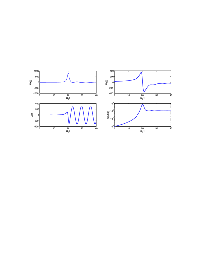
Figure 1: The evolution of a single SFH when initial conditions correspond to the tightly leading pure vortex mode. Velocity components ($v_{x}(t)k_{H}/\Omega_{0}$, $v_{y}(t)k_{H}/\Omega_{0}$, $v_{z}(t)k_{H}/\Omega_{0}$,) and normalized energy of perturbation SFH ($E_{k}(t)/E(0)$) are shown. Here $\leavevmode\nobreak\ k_{x}(0)/k_{y}=-30$, $\leavevmode\nobreak\ k_{y}=k_{z}=10k_{H}$.

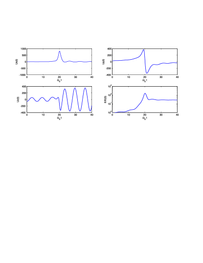
Figure 2: Same as Fig. 1, but when the initial conditions for the single SFH correspond to a mix of vortex and SDW modes. Note that the differences are rather minor, since the vortex mode dominates.

To impose initially pure vortex mode perturbations, we use approximate solutions that can be derived from Eq. (38):

$$\Phi_{0}(t)={f_{\phi}(t)\over\omega_{\phi}^{2}(t)}W\leavevmode\nobreak\ .$$ (41)

This solution describes a vortex mode when the temporal variation of the vortical perturbations is much slower than the SDW oscillations. Hence, we start our numerical integration of Eqs. (28-31) at wavenumbers where the above condition is amply satisfied, i.e., at $|k_{x}(0)/k_{y}|\gg 1$.

Figure 1 displays the evolution of a dynamically active $(k_{y}=k_{z})$ single SFH when the initial conditions correspond to a tightly leading pure vortex mode $\leavevmode\nobreak\ (k_{x}(0)/k_{y}=-30)$. We see that in the leading phase only that vortex mode is present. Oscillations (hence wave SFH) appear in the trailing phase after time $t=t^{*}=20/\Omega_{0}$ when $k_{x}(t)=0$. The SDW oscillates mainly in the vertical direction; thus oscillations are the most pronounced in $v_{z}$. The graph of the density $D$ is similar to that of $v_{z}$ and so is not presented here. The energy graph shows the transient growth in the leading phase. In the trailing phase, the generated wave SFH keeps the energy (since SDW do not exchange the energy with the mean flow). This course of events – the transient growth and subsequent coupling – makes the energy dynamics similar to the 3D unbounded plane Couette flow case. Note that the tighter the initial leading SFH is, i.e. the higher the ratio $|k_{x}(0)/k_{y}|$, the stronger the transient growth. The possible maximum value of $|k_{x}(0)/k_{y}|$ is determined by the Reynolds number ($Re$). Consequently, the amplification factor is determined by $\leavevmode\nobreak\ Re\leavevmode\nobreak\$ and it can become huge since in Keplerian disks $Re$ reaches literally astronomical values $(Re>10^{10})\leavevmode\nobreak\$ (see Sect. 3 of T03 for details).

Imposing a leading SFH ($k_{x}(0)/k_{y}<0$) of pure wave mode, we do not detect any notable transient growth in the wave SFH, or any generation of the vortex mode: since the potential vorticity is time invariant (see Eq. 26), the wave SFH, having zero potential vorticity, is not able to generate the vortex SFH, which has non-zero potential vorticity. Hence, waves with zero potential vorticity alone, which were also recently described by Goodman and Balbus (2001), are not expected to support energetically hydrodynamic turbulence in Keplerian flows.

Figure 2 shows the evolution of another dynamically active single SFH with $k_{y}=k_{z}$, again with $k_{x}(0)/k_{y}=-30$, but where the initial conditions correspond to a mix of vortex and SDW modes. The initial admixture of the wave SFH does not change the dynamic picture qualitatively, due to the already mentioned reason, that SDW does not exchange energy with the mean flow. The energy graph is similar to Fig. 7 of Brandenburg & Dintrans (2006), though the linear mode coupling has not been identified there.

Let us concentrate on the linear dynamics when we initially insert a tightly leading SFH of vortex mode perturbation. The dynamics is then the most complex and the energy exchange the most efficient, due both to the transient growth of the SFH and to mode coupling with the SDW. The intensity of these processes depends on values of $k_{x}(0)/k_{y}$ and $k_{z}/k_{y}$.

The ratio $E_{k}(t^{*})/E(0)$ gives a good estimate of the nonmodal growth of vortex SFHs. Here, $t^{*}$ is the time when $k_{x}(t^{*})=0$. The spectral behavior (specifically, the dependence on $k_{z}/k_{y}$) of the transient amplification rate calculated by Eqs. (28-31) is shown in the left panel of Fig. 3. A constant value of $k_{x}(0)/k_{y}=-30$ is chosen to simulate the energy growth of vortex perturbations at constant Reynolds number. One can see that the transient amplification is efficient at low values of $k_{z}$, while it is strongly reduced for SFHs with $k_{z}\gg k_{y}$.

The right panel of Fig. 3 shows the mode coupling efficiency, measured in units $E_{k}(wave)/E(0)$, vs $k_{z}/k_{y}$, where $E_{k}(wave)$ is the final energy of the wave SFH ($E_{k}(wave)=E(t_{fin})-E(0)$, $t_{fin}=2t^{*}=40\Omega_{0}$). That efficiency has a pronounced maximum at $k_{z}\simeq k_{y}$. The energy of the amplified vortex SFH is transformed into the wave SHF due to mode coupling, so at later times, the main carrier of the perturbation energy is the SDW (since vortex decay in the trailing phase, while waves evolve keeping nearly constant energy). Therefore, SFHs with $k_{z}\sim k_{y}$ are dynamically active and should play an important role in the turbulent process. These wavenumbers were chosen in Figs. 1-2 to show the dynamical picture of these SFHs and illustrate the significance of the transient growth and subsequent mode coupling.

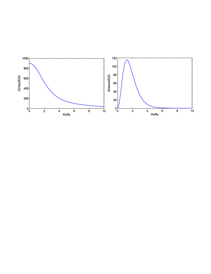
Figure 3: Left: energy amplification through transient growth of vortex mode perturbations ${\rm Max}(E(t)/E(0))$ vs. $k_{z}/k_{y}$.       Right: mode coupling efficiency measured by the generated wave energy $E(wave)/E(0)$ vs. $k_{z}/k_{y}$. Here $k_{x}(0)/k_{y}=-30$, $k_{y}=10k_{H}$ and the maximum efficiency of mode coupling is achieved at $k_{z}/k_{y}=1.25$.

In Fig. 4 we have chosen the phase space to display the evolution of the vertical and total velocities. The initial conditions correspond to the pure vortex mode (top row, $A.1$ and $A.2$) and a mix of vortex and wave modes (bottom row, $B.1$ and $B.2$) presented in Figs. 3 and 4. The initial point is marked by a triangle, and the point at which $\leavevmode\nobreak\ k_{x}(t)=0\leavevmode\nobreak\$ is marked by a circle. The segments from triangle to circle in the top row graphs describe the transient growth of the leading phase of the vortex mode. In the trailing phase, after the circle marker, one can see some subsiding of the vortex harmonic and generation of the wave (due to mode coupling). The latter is indicated by the cyclic phase trajectories. The persistence of cyclic trajectories illustrates the constancy of the wave SFH energy: the wave is the main carrier of the perturbation energy at later times. The bottom graphs show that the mix of initial vortex and wave harmonics evolves much in the same manner. Differences are seen initially, before the vortex has undergone transient growth. The graph $B.1$ shows the transient growth and mode coupling in phase space in terms of the vertical velocity. Note how the initial “low level” cyclic phase trajectories are transformed into “high level” cyclic trajectories by transient growth of the vortex admixture and the subsequent generation of the wave harmonic by the vortex mode. It illustrates how transient growth raises a perturbation to a higher energy state.

The vortex mode undergoes the amplification or damping depending on its phase (leading or trailing) in differentially rotating flows. From this, it has been speculated (see Johnson & Gammie 2005) that any realistic ensemble of these modes covering a wide area in wave-number space will not exhibit cumulative energy growth. However, as we have seen in Figs. 1-2 total energy of the SFH exhibits asymmetry in growth and decay, due to the mode coupling. Hence, any ensemble of initial perturbations that include vortex mode perturbations and cover the region $k_{z}\sim k_{y}$ will undergo overall energy growth in time.

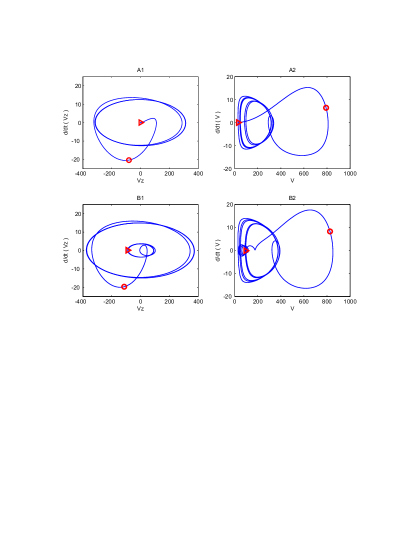
Figure 4: The vertical velocity (panels $A.1$ and $B.1$) and total velocity amplitude (panels $A.2$ and $B.2$) of perturbations in phase space (${\rm v}$, ${\rm dv/d}t$). Top row shows the evolution of perturbations when initial conditions correspond to the vortex mode (panels $A.1$ and $A.2$), while a mix of vortex and wave modes is shown in the bottom row (panels $B.1$ and $B.2$). A triangle marks the initial state, while the circle corresponds to the time when $k_{x}(t)=0$.

4 Discussion

Our motivation in studying mode coupling in the presence of vertical stratification is quite clear: in unstratified rotating flows the strato-rotational balance is absent (see Eq. 35), hence there will be no vortex mode, whose role is so powerful in extracting the shear flow energy. Moreover, in stratified rotating flows mode coupling causes the generation of SDW, which are able to conserve the extracted energy. Thus one expects astrophysical disks, which are vertically stratified, to demonstrate intrinsically different behavior compared to unstratified rotating flows. Therefore it is not possible to draw conclusions about the stability of astrophysical disks by considering unstratified rotating flows, as has been done often in the past and again in recent investigations: analytical (Balbus 2006), numerical (Shen et al. 2006), and experimental (Ji et al. 2006).

Our analysis shows that, in the local limit, spectrally stable stratified Keplerian disks allow for two modes of perturbations – vortex and SDW – that are jointly able to extract the background flow energy and determine the disk dynamical activity in the small-scale range. These modes are linearly coupled due to the non-normality of Keplerian/shear flow. The coupling is asymmetric: the vortex mode is able to generate the related SDW, but the inverse is not true. This mode coupling is transient (like the energy exchange between perturbations and the basic flow): the SFH of the vortex mode generates the wave SFHs during the brief time interval where it switches from leading to trailing, thus rendering the dynamics non-adiabatic.

At first sight, the mode coupling described here seems similar to the phenomenon of geostrophic adjustment, since both lead to the generation of the spiral density waves. However, these processes are intrinsically different. Geostrophic adjustment is an initial value problem that describes the transition from an initially unbalanced state to that of geostrophic balance. In the general case, part of the initial conditions containing no potential vorticity (the wave component) will radiate away as inertial-gravity waves (see, e.g., Pedlosky 2003) during the geostrophic adjustment, whereas our initial conditions do not include zero potential vorticity corresponding to the wave component. Hence, we have eliminated the wave generation due to the process of the initial geostropic adjustment. The waves generated in our case stem from linear mode coupling induced by the velocity shear. Moreover, geostrophic adjustment is mainly a nonlinear process that leads to equilibrium. In contrast, wave generation due to mode coupling is a linear process and does not describe the relaxation of the system, but hopefully the opposite: it promotes the transition to turbulence.

The linear dynamics of each leading SFH of vortex mode proceeds in the following way: initially, the SFH extracts energy from the basic flow and it grows. At the same time $\leavevmode\nobreak\ k_{x}(t)/k_{y}\to-0$. Becoming trailing, the vortex SFH generates the related SFH of SDW. In what follows, while tilting (i.e., increasing $\leavevmode\nobreak\ k_{x}(t)/k_{y}$), the wave SFH keeps the energy, whereas the vortex SFH gives its energy back to the basic flow, so the energy gained by the leading vortex SFH is conserved by the SDW. This course of events – the transient growth plus coupling – is strongly pronounced for SFHs with $\leavevmode\nobreak\ k_{z}/k_{y}\sim 1$ and makes their energy dynamics similar to that of a 3D unbounded plane Couette flow.

We are aware that there are differences between them: in the Couette case, only the vortex mode participates in the dynamical process, whereas in the disk case, this role is played (in the local limit) by the symbiosis between vortex and SDW perturbations. However, given the similarities that we have discussed, we conjecture that the bypass concept, which has been developed for the transition to turbulence in the Couette flow, is also applicable to rotating stratified disks. One question remains, of course: will the nonlinear interactions provide positive feedback that is efficient enough for that bypass transition? To answer it, more numerical simulations are needed, which must include the vertical stratification and grasp the mode coupling.