Thermodynamic time asymmetry in nonequilibrium fluctuations

Abstract

We here present the complete analysis of experiments on driven Brownian motion and electric noise in a $RC$ circuit, showing that thermodynamic entropy production can be related to the breaking of time-reversal symmetry in the statistical description of these nonequilibrium systems. The symmetry breaking can be expressed in terms of dynamical entropies per unit time, one for the forward process and the other for the time-reversed process. These entropies per unit time characterize dynamical randomness, i.e., temporal disorder, in time series of the nonequilibrium fluctuations. Their difference gives the well-known thermodynamic entropy production, which thus finds its origin in the time asymmetry of dynamical randomness, alias temporal disorder, in systems driven out of equilibrium.

I Introduction

According to the second law of thermodynamics, nonequilibrium systems produce entropy in a time asymmetric way. This thermodynamic time asymmetry is usually expressed in terms of macroscopic concepts such as entropy. The lack of understanding of this time asymmetry in terms of concepts closer to the microscopic description of the motion of particles has always been a difficulty. Only recently, general relationships have been discovered which allows us to express the thermodynamic time asymmetry at the mesoscopic level of description in terms of the probabilities ruling the molecular or thermal fluctuations in nonequilibrium systems. More specifically the entropy production rate in a system driven out of equilibrium can be estimated by measuring the asymmetries between the probabilities of finding certain time evolutions when the system is driven with forward nonequilibrium driving and those of finding the corresponding reversed time evolutions with a backward driving. In a recent letter AGCGJP07 , experimental evidence has been reported that, indeed, the entropy production finds its origin in the time asymmetry of the dynamical randomness, alias temporal disorder, in driven Brownian motion and in the electric noise of a driven $RC$ circuit. In these two experiments we record long time series, either of the position of the Brownian particle or of the fluctuating voltage of the $RC$ circuits, which allow us to define the probabilities of given time evolutions, also called paths. This result shows that, under nonequilibrium conditions, the probabilities of the direct and time-reversed paths break the time-reversal symmetry and that the entropy production is given by the difference between the decay rates of these probabilities. These decay rates characterize the dynamical randomness of the paths (or their time reversals) so that the entropy production turns out to be directly related to the breaking of the time-reversal symmetry in the dynamical randomness of the nonequilibrium fluctuations.

The purpose of the present paper is to provide a detailed report of these two experiments and of the data analysis. The dynamical randomness of the forward time series is characterized by the so-called $(\varepsilon,\tau)$-entropy per unit time, which represents the average decay rate of the probabilities of paths sampled with a resolution $\varepsilon$ and a sampling time $\tau$ GW93 . The precise definition of these quantities will be given in Sec. III. To each possible path in the forward time series, we look for the corresponding time-reversed path in the backward time series. This allows us to further obtain the time-reversed $(\varepsilon,\tau)$-entropy per unit time. Remarkably, the difference between the backward and forward $(\varepsilon,\tau)$-entropies per unit time gives the right positive value of the thermodynamic entropy production under nonequilibrium conditions. This result shows by direct data analysis that the entropy production of nonequilibrium thermodynamics can be explained as a time asymmetry in the temporal disorder characterized by these new quantities which are the $(\varepsilon,\tau)$-entropies per unit time.

These quantities were introduced in order to generalize the concept of Kolmogorov-Sinai entropy per unit time from dynamical systems to stochastic processes GW93 ; ER85 . In this regard, the relationship here described belongs to the same family of newly discovered large-deviation properties as the escape-rate and chaos-transport formulas GN90 ; DG95 ; GCGD01 , the steady-state or transient fluctuation theorems ECM93 ; ES94 ; GC95 ; K98 ; LS99 ; M99 ; MN03 ; W02 ; ZC03 ; ZCC04 ; GC04 ; DJGPC06 ; SSTWS05 ; S05 ; TC06 ; HS07 ; AG07a ; AG07b , and the nonequilibrium work fluctuation theorem C99 ; DCP05 ; CRJSTB05 ; J06 ; KPV07 . All these relationships share the common mathematical structure that they give an irreversible property as the difference between two decay rates of mesoscopic or microscopic properties G05 ; G06 . These relationships are at the basis of the important advances in nonequilibrium statistical mechanics during the last two decades DGV07 . Recently, the concept of time-reversed entropy per unit time was introduced G04 and used to express the thermodynamic entropy production in terms of the difference between it and the standard (Kolmogorov-Sinai) entropy per unit time G05 ; G04 ; LAvW05 ; NVdS06 . This relationship can be applied to probe the time asymmetry of time series AGCGJP07 ; PRD07 and allows us to understand the origin of the thermodynamic time asymmetry.

The paper is organized as follows. In Sec. II, we introduce the Langevin description of the experiments. In particular, we show that the thermodynamic entropy production arises from the breaking of the forward and time-reversed probability distributions over the trajectories. In Sec. III, we introduce the dynamical entropies and describe an algorithm for their estimation using long time series. It is shown that the difference between the two dynamical entropies gives back the thermodynamic entropy production. The experimental results on driven Brownian motion are presented in Sec. IV where we analyze in detail the behavior of the dynamical entropies and establish the connection with the thermodynamic entropy production. The experimental results on electric noise in the driven $RC$ circuit are given in Sec. V. The relation to the extended fluctuation theorem ZC03 ; ZCC04 ; GC04 is discussed in Sec. VI. The conclusions are drawn in Sec. VII.

II Stochastic description, path probabilities, and entropy production

We consider a Brownian particle in a fixed optical trap and surrounded by a fluid moving at the speed $u$. In a viscous fluid such as water solution at room temperature and pressure, the motion of a dragged micrometric particle is overdamped. In this case, its Brownian motion can be modeled by the following Langevin equation ZCC04 :

$$\alpha\frac{dz}{dt}=F(z)+\alpha u+\xi_{t}$$ (1)

where $\alpha$ is the viscous friction coefficient, $F=-\partial_{z}V$ the force exerted by the potential $V$ of the laser trap, $\alpha u$ is the drag force of the fluid moving at speed $u$, and $\xi_{t}$ a Gaussian white noise with its average and correlation function given by

$$\langle\xi_{t}\rangle = 0$$ (2)

$$\langle\xi_{t}\,\xi_{t^{\prime}}\rangle = 2\,k_{\rm B}T\,\alpha\,\delta(t-t^{\prime})$$ (3)

In the special case where the potential is harmonic of stiffness $k$, $V=kz^{2}/2$, the stationary probability density is Gaussian

$$p_{\rm st}(z)=\sqrt{\frac{\beta k}{2\pi}}\exp\Big{[}-\frac{\beta k}{2}(z-u\,\tau_{R})^{2}\Big{]}$$ (4)

with the relaxation time

$$\tau_{R}=\frac{\alpha}{k}$$ (5)

and the inverse temperature $\beta=(k_{\rm B}T)^{-1}$. The maximum of this Gaussian distribution is located at the distance $u\tau_{R}$ of the minimum of the confining potential. This shift is due to dragging and corresponds to the position where there is a balance between the frictional and harmonic forces.

The work $W_{t}$ done on the system by the moving fluid during the time interval $t$ is given by ZC03 ; ZCC04 ; S97

$$W_{t}=-\int_{0}^{t}u\;F(z_{t^{\prime}})\;dt^{\prime}$$ (6)

while the heat $Q_{t}$ generated by dissipation is

$$Q_{t}=\int_{0}^{t}\left(\dot{z}_{t^{\prime}}-u\right)\;F(z_{t^{\prime}})\;dt^{\prime}$$ (7)

We notice that the quantities (6) and (7) are fluctuating because of the Brownian motion of the particle. Both quantities are related by the change in potential energy $\Delta V_{t}\equiv V(z_{t})-V(z_{0})$ so that

$$Q_{t}=W_{t}-\Delta V_{t}$$ (8)

In a stationary state, the mean value of the dissipation rate is equal to the mean power done by the moving fluid since $\lim_{t\to\infty}(1/t)\langle\Delta V_{t}\rangle=0$. The thermodynamic entropy production is thus given by

$$\frac{d_{\rm i}S}{dt}=\lim_{t\to\infty}\frac{1}{t}\frac{\langle Q_{t}\rangle}{T}=\lim_{t\to\infty}\frac{1}{t}\frac{\langle W_{t}\rangle}{T}=\frac{\alpha u^{2}}{T}$$ (9)

in the stationary state. The equilibrium state is reached when the speed of the fluid is zero, $u=0$, in which case the entropy production (9) vanishes as expected.

An equivalent system is an $RC$ electric circuit driven out of equilibrium by a current source which imposes the mean current $I$ ZCC04 ; GC04 . The current fluctuates in the circuit because of the intrinsic Nyquist thermal noise. This electric circuit and the dragged Brownian particle, although physically different, are known to be formally equivalent by the correspondence shown in Table 1 ZCC04 .

Brownian particle $RC$ circuit $z_{t}$ $q_{t}-It$ $\dot{z}_{t}$ $\dot{q}_{t}-I$ $\xi_{t}$ $-\delta V_{t}$ $\alpha$ $R$ $k$ $1/C$ $u$ $-I$

Table 1: The analogy between the Brownian particle and the electric $RC$ circuit. For the Brownian particle, $z_{t}$ is its position, $\dot{z}_{t}$ its velocity, $\xi_{t}$ the Langevin fluctuating force, $\alpha$ the viscous friction coefficient, $k$ the harmonic strength or stiffness of the optical trap, and $u$ the fluid speed. For the electric circuit, $q_{t}$ is the electric charge passing through the resistor during time $t$, $i_{t}=\dot{q}_{t}$ the corresponding current, $\delta V_{t}$ the fluctuating electric potential of the Nyquist noise, $R$ the resistance, $C$ the capacitance, and $I$ the mean current source.

Our aim is to show that one can extract the heat dissipated along a fluctuating path by comparing the probability of this path, with the probability of the corresponding time-reversed path having also reversed the external driving, i.e., $u\rightarrow-u$ for the dragged Brownian particle (respectively, $I\to-I$ for the $RC$ circuit).

We use a path integral formulation. A stochastic trajectory is uniquely defined by specifying the noise history of the system $\xi_{t}$. Indeed, the solution of the stochastic equation (1), i.e.,

$$z_{t} = z_{0}+\int_{0}^{t}\;dt^{\prime}\;\dot{z}_{t^{\prime}}$$ (10)

$$= z_{0}+\frac{1}{\alpha}\int_{0}^{t}\;dt^{\prime}\;\Big{[}F(z_{t^{\prime}})+\alpha u+\xi_{t^{\prime}}\Big{]}$$

is uniquely specified if the noise history is known. Since we consider a Gaussian white noise, the probability to have the noise history $\xi_{t}$ is given by OM53

$$P[\xi_{t}]\propto\exp\left[-\frac{1}{4k_{\rm B}T\alpha}\int_{0}^{t}\;dt^{\prime}\;\big{(}\xi_{t^{\prime}}\big{)}^{2}\right]$$ (11)

According to Eq. (1), the probability of a trajectory $z_{t}$ starting from the fixed initial point $z_{0}$ is thus written as

$$P[z_{t}|z_{0}]\propto\exp\left[-\frac{1}{4k_{\rm B}T\alpha}\int_{0}^{t}\;dt^{\prime}\;\Big{(}\alpha\dot{z}-F(z)-\alpha u\Big{)}^{2}\right]$$ (12)

We remark that the corresponding joint probability is obtained by multiplying the conditional probability (12) with the stationary probability density (4) of the initial position as

$$P[z_{t}]\propto P[z_{t}|z_{0}]\,p_{\rm st}(z_{0})$$ (13)

To extract the heat dissipated along a trajectory, we consider the probability of a given path over the probability to observe the reversed path having also reversed the sign of the driving $u$. The reversed path is thus defined by $z_{t^{\prime}}^{\rm R}=z_{t-t^{\prime}}$ which implies $\dot{z}_{t^{\prime}}^{\rm R}=-\dot{z}_{t-t^{\prime}}$. Therefore, we find that

$$\ln\frac{P_{+}[z_{t}|z_{0}]}{P_{-}[z_{t}^{\rm R}|z_{0}^{\rm R}]} = -\frac{1}{4k_{\rm B}T\alpha}\int_{0}^{t}\;dt^{\prime}\;\left[\Big{(}\alpha\dot{z}-F(z)-\alpha u\Big{)}^{2}-\Big{(}-\alpha\dot{z}-F(z)+\alpha u\Big{)}^{2}\right]$$ (14)

$$= \frac{1}{k_{\rm B}T}\int_{0}^{t}\;dt^{\prime}\;\Big{(}\dot{z}-u\Big{)}\;F(z)$$

$$= \frac{1}{k_{\rm B}T}\left[V(z_{0})-V(z_{t})-u\int_{0}^{t}\;dt^{\prime}\;F(z)\right]$$

$$= \frac{Q_{t}}{k_{\rm B}T}$$

which is precisely the fluctuating heat (7) dissipated along the random path $z_{t}$ and expressed in the thermal unit $k_{\rm B}T$. The detailed derivation of this result is carried out in Appendix A. The dissipation can thus be related to time-symmetry breaking already at the level of mesoscopic paths. We notice that the mean value of the fluctuating quantity (14) behaves as described by Eq. (9) so that the heat dissipation rate vanishes on average at equilibrium and is positive otherwise. Relations similar to Eq. (14) are known for Boltzmann’s entropy production MN03 , for time-dependent systems S05 ; C99 ; KPV07 , and in the the context of Onsager-Machlup theory TC06 . We emphasize that the reversal of $u$ is essential to get the dissipated heat from the way the path probabilities $P_{+}$ and $P_{-}$ differ.

The main difference between these path probabilities comes from the shift between the mean values of the fluctuations under forward or backward driving. Indeed, the average position is equal to $\langle z\rangle_{+}=u\tau_{R}$ under forward driving at speed $+u$, and $\langle z\rangle_{-}=-u\tau_{R}$ under backward driving at speed $-u$. The shift $2u\tau_{R}$ in the average positions implies that a typical path of the forward time series falls, after its time reversal, in the tail of the probability distribution $P_{-}$ of the backward time series. Therefore, the probabilities $P_{-}$ of the time-reversed forward paths in the backward time series are typically lower than the probabilities $P_{+}$ of the corresponding forward paths. The above derivation (14) shows that the dissipation can be obtained in terms of their ratio $P_{+}/P_{-}$. We emphasize that this derivation holds for anharmonic potentials as well as harmonic ones, so that the result is general in this respect.

In the stationary state, the mean entropy production (9) is given by averaging the dissipated heat (14) over all possible trajectories:

$$\frac{d_{\rm i}S}{dt} = \lim_{t\to\infty}\frac{k_{\rm B}}{t}\left\langle\ln\frac{P_{+}[z_{t}|z_{0}]}{P_{-}[z_{t}^{\rm R}|z_{0}^{\rm R}]}\right\rangle$$ (15)

$$= \lim_{t\to\infty}\frac{k_{\rm B}}{t}\left\langle\ln\frac{P_{+}[z_{t}]}{P_{-}[z_{t}^{\rm R}]}\right\rangle$$

$$= \lim_{t\to\infty}\frac{k_{\rm B}}{t}\int{\cal D}z_{t}\;P_{+}[z_{t}]\;\ln\frac{P_{+}[z_{t}]}{P_{-}[z_{t}^{\rm R}]}\ \geq\ 0$$

The second equality in Eq. (15) results from the fact that the terms at the boundaries of the time interval $t$ are vanishing for the statistical average in the long-time limit. Equation (15) relates the thermodynamic dissipation to a so-called Kullback-Leibler distance KL51 or relative entropy W78 between the forward process and its time reversal. Such a connection between dissipation and relative entropy has also been described elsewhere J06 ; KPV07 ; G04 . Since the relative entropy is known to be always non negative, the mean entropy production (15) satisfies the second law of thermodynamics, as it should. Accordingly, the mean entropy production vanishes at equilibrium because of Eq. (9) or, equivalently, as the consequence of detailed balance which holds at equilibrium when the speed $u$ is zero (see Appendix A).

We point out that the heat dissipated along an individual path given by Eq. (14) is a fluctuating quantity and may be either positive or negative. We here face the paradox raised by Maxwell that the dissipation is non-negative on average but has an undetermined sign at the level of the individual stochastic paths. The second law of thermodynamics holds for entropy production defined after statistical averaging with the probability distribution. We remain with fluctuating mechanical quantities at the level of individual mesoscopic paths or microscopic trajectories.

III Dynamical randomness and thermodynamic entropy production

The aim of this section is to present a method to characterize the property of dynamical randomness in the time series and to show how this property is related to the thermodynamic entropy production when the paths are compared with their time reversals. In this way, we obtain a theoretical prediction on the relationship between dynamical randomness and thermodynamic entropy production.

III.1 $(\varepsilon,\tau)$-entropies per unit time

Dynamical randomness is the fundamental property of temporal disorder in the time series. The temporal disorder can be characterized by an entropy as well as for the other kinds of disorder. In the case of temporal disorder, we have an entropy per unit time, which is the rate of production of information by the random process, i.e., the minimum number of bits (digits or nats) required to record the time series during one time unit. For random processes which are continuous in time and in their variable, the trajectories should be sampled with a resolution $\varepsilon$ and with a sampling time $\tau$. Therefore, the entropy per unit time depends a priori on each one of them and we talk about the $(\varepsilon,\tau)$-entropy per unit time. Such a quantity has been introduced by Shannon as the rate of generating information by continuous sources S48 . The theory of this quantity was developed under the names of $\varepsilon$-entropy K56 and rate distortion function B71 . More recently, the problem of characterizing dynamical randomness has reappeared in the study of chaotic dynamical systems. A numerical algorithm was proposed by Grassberger, Procaccia and coworkers GP83 ; CP85 in order to estimate the Kolmogorov-Sinai entropy per unit time. Thereafter, it was shown that the same algorithm also applies to stochastic processes, allowing us to compare the property of dynamical randomness of different random processes GW93 ; G98 . Moreover, these dynamic entropies were measured for Brownian motion at equilibrium GBFSGDC98 ; BSFGGDC01 . We here present the extension of this method to out-of-equilibrium fluctuating systems.

Since we are interested in the probability of a given succession of states obtained by sampling the signal $Z(t)$ at small time intervals $\tau$, a multi-time random variable is defined according to ${\textbf{\em Z}}=[Z(t_{0}),Z(t_{0}+\tau),\ldots,Z(t_{0}+n\tau-\tau)]$, which represents the signal during the time period $t-t_{0}=n\tau$. For a stationary process, the probability distribution does not depend on the initial time $t_{0}$. From the point of view of probability theory, the process is defined by the $n$-time joint probabilities

$$P_{s}({\textbf{\em z}};d{\textbf{\em z}},\tau,n)={\rm Pr}\{{\textbf{\em z}}<{\textbf{\em Z}}<{\textbf{\em z}}+d{\textbf{\em z}};s\}=p_{s}({\textbf{\em z}})\,d{\textbf{\em z}}$$ (16)

where $p_{s}({\textbf{\em z}})$ denotes the probability density for Z to take the values ${\textbf{\em z}}=(z_{0},z_{1},\ldots,z_{n-1})$ at times $t_{0}+i\tau$ ($i=0,1,2,...,n-1$) for some nonequilibrium driving $s=u/|u|=\pm 1$. Now, due to the continuous nature in time and in space of the process, we will consider the probability $P_{+}({\textbf{\em Z}}_{m};\varepsilon,\tau,n)$ for the trajectory to remain within a distance $\varepsilon$ of some reference trajectory ${\textbf{\em Z}}_{m}$, made of $n$ successive positions of the Brownian particle observed at time intervals $\tau$ during the forward process. This reference trajectory belongs to an ensemble of $M$ reference trajectories $\{{\textbf{\em Z}}_{m}\}_{m=1}^{M}$, allowing us to take statistical averages. These reference trajectories define the patterns, i.e., the recurrences of which are searched for in the time series.

On the other hand, we can introduce the quantity $P_{-}({\textbf{\em Z}}^{\rm R}_{m};\varepsilon,\tau,n)$ which is the probability for a reversed trajectory of the reversed process to remain within a distance $\varepsilon$ of the reference trajectory ${\textbf{\em Z}}_{m}$ (of the forward process) for $n$ successive positions.

Suppose we have two realizations over a very long time interval $L\tau\gg n\tau$ given by the time series $\{z_{\pm}(k\tau)\}_{k=1}^{L}$, respectively for the forward ($+$) and backward ($-$) processes. Within these long time series, sequences of length $n$ are compared with each other. We thus consider an ensemble set of $1\ll M\ll L$ reference sequences, which are all of length $n$:

$${\textbf{\em Z}}_{m}=[Z(m\tau),\cdots,Z(m\tau+n\tau-\tau)],\quad m\in\{m_{1},\cdots,m_{M}\}$$ (17)

These reference sequences are taken at equal time intervals in order to sample the forward process according to its probability distribution $P_{+}$. The distance between a reference sequence and another sequence of length $n$ is defined by

$${\rm dist}_{n}({\textbf{\em Z}}_{m},{\textbf{\em Z}}_{j})=\max\{|Z(m\tau)-Z(j\tau)|,\cdots,|Z(m\tau+n\tau-\tau)-Z(j\tau+n\tau-\tau)|\}$$ (18)

for $j=1,2,...,L^{\prime}=L-n+1$. The probability for this distance to be smaller than $\varepsilon$ is then evaluated by

$$P_{+}({\textbf{\em Z}}_{m};\varepsilon,\tau,n)=\frac{1}{L^{\prime}}\ {\rm Number}\{{\textbf{\em Z}}_{j}:{\rm dist}_{n}({\textbf{\em Z}}_{m},{\textbf{\em Z}}_{j})\leq\varepsilon\}$$ (19)

The average of the logarithm of these probabilities over the different reference sequences gives the block entropy

$$H(\varepsilon,\tau,n)=-\frac{1}{M}\sum_{m=1}^{M}\ln P_{+}({\textbf{\em Z}}_{m};\varepsilon,\tau,n)$$ (20)

also called the mean pattern entropy. The ($\varepsilon,\tau$)-entropy per unit time is then defined as the rate of the linear growth of the block entropy as the length $n$ of the reference sequences increases GW93 ; GP83 ; CP85 :

$$h(\varepsilon,\tau)=\lim_{n\rightarrow\infty}\lim_{L^{\prime},M\rightarrow\infty}\frac{1}{\tau}\Big{[}H(\varepsilon,\tau,n+1)-H(\varepsilon,\tau,n)\Big{]}$$ (21)

Similarly, the probability of a reversed trajectory in the reversed process can be evaluated by

$$P_{-}({\textbf{\em Z}}_{m}^{\rm R};\varepsilon,\tau,n)=\frac{1}{L^{\prime}}\ {\rm Number}\{\tilde{\textbf{\em Z}}_{j}:{\rm dist}_{n}({\textbf{\em Z}}_{m}^{\rm R},\tilde{\textbf{\em Z}}_{j})\leq\varepsilon\}$$ (22)

where ${\textbf{\em Z}}_{m}^{\rm R}=[Z(m\tau+n\tau-\tau),\cdots,Z(m\tau)]$ is the time reversal of the reference path ${\textbf{\em Z}}_{m}$ of the forward process, while $\{\tilde{\textbf{\em Z}}_{j}\}_{j=1}^{L^{\prime}}$ are the paths of the reversed process (with the opposite driving $-u$). In similitude with Eqs. (20) and (21), we may introduce the time-reversed block entropy:

$$H^{\rm R}(\varepsilon,\tau,n)=-\frac{1}{M}\sum_{m=1}^{M}\ln P_{-}({\textbf{\em Z}}^{\rm R}_{m};\varepsilon,\tau,n)$$ (23)

and the time-reversed ($\varepsilon,\tau$)-entropy per unit time:

$$h^{\rm R}(\varepsilon,\tau)=\lim_{n\rightarrow\infty}\lim_{L^{\prime},M\rightarrow\infty}\frac{1}{\tau}\Big{[}H^{\rm R}(\varepsilon,\tau,n+1)-H^{\rm R}(\varepsilon,\tau,n)\Big{]}$$ (24)

We notice that the dynamical entropy (21) gives the decay rate of the probabilities to find paths within a distance $\varepsilon$ from a typical path ${\textbf{\em Z}}=(Z_{0},Z_{1},Z_{2},...,Z_{n-1})$ with $Z_{i}=Z(t_{0}+i\tau)$:

$$P_{+}({\textbf{\em Z}};\varepsilon,\tau,n)\sim\exp[-n\tau h(\varepsilon,\tau)]\qquad(n\to\infty)$$ (25)

as the number $n$ of time intervals increases. In the case of ergodic random processes, this property is known as the Shannon-McMillan-Breiman theorem B65 . The decay rate $h$ characterizes the temporal disorder, i.e., dynamical randomness, in both deterministic dynamical systems and stochastic processes GW93 ; ER85 ; GP83 ; CP85 ; G98 . On the other hand, the time-reversed dynamical entropy (24) is the decay rate of the probabilities of the time-reversed paths in the reversed process:

$$P_{-}({\textbf{\em Z}}^{\rm R};\varepsilon,\tau,n)\sim\exp[-n\tau h^{\rm R}(\varepsilon,\tau)]\qquad(n\to\infty)$$ (26)

Since $h^{\rm R}$ is the decay rate of the probability to find, in the backward process, the time-reversed path corresponding to some typical path of the forward process, the exponential $\exp(-h^{\rm R}\Delta t)$ evaluates the amount of time-reversed paths among the typical paths (of duration $\Delta t$). The time-reversed entropy per unit time $h^{\rm R}$ thus characterizes the rareness of the time-reversed paths in the forward process.

The dynamical randomness of the stochastic process ruled by the Langevin equation (1) can be characterized in terms of its $(\varepsilon,\tau)$-entropy per unit time. This latter is calculated for the case of a harmonic potential in Appendix B. For small values of the spatial resolution $\varepsilon$, we find that

$$h(\varepsilon,\tau)=\frac{1}{\tau}\ln\sqrt{\frac{\pi{\rm e}D\tau_{R}}{2\varepsilon^{2}}\left(1-{\rm e}^{-2\tau/\tau_{R}}\right)}+O(\varepsilon^{2})$$ (27)

with the diffusion coefficient of the Brownian particle:

$$D=\frac{k_{\rm B}T}{\alpha}$$ (28)

The $(\varepsilon,\tau)$-entropy per unit time increases as the resolution $\varepsilon$ decreases, meaning that randomness is found on smaller and smaller scales in typical trajectories of the Brownian particle. After having obtained the main features of the $(\varepsilon,\tau)$-entropy per unit time, we go on in the next subsection by comparing it with the time-reversed $(\varepsilon,\tau)$-entropy per unit time, establishing the connection with thermodynamics.

III.2 Thermodynamic entropy production

Under nonequilibrium conditions, detailed balance does not hold so that the probabilities of the paths and their time reversals are different. Similarly, the decay rates $h$ and $h^{\rm R}$ also differ. Their difference can be calculated by evaluating the path integral (15) by discretizing the paths with the sampling time $\tau$ and resolution $\varepsilon$

$$\frac{d_{\rm i}S}{dt} = \lim_{t\to\infty}\frac{k_{\rm B}}{t}\int{\cal D}z_{t}\;P_{+}[z_{t}]\;\ln\frac{P_{+}[z_{t}]}{P_{-}[z_{t}^{\rm R}]}$$ (29)

$$= \lim_{\varepsilon\rightarrow 0}\lim_{\tau\rightarrow 0}\lim_{n\rightarrow\infty}\lim_{L^{\prime},M\rightarrow\infty}\frac{k_{\rm B}}{n\tau}\frac{1}{M}\sum_{m=1}^{M}\ln\frac{P_{+}({\textbf{\em Z}}_{m};\varepsilon,\tau,n)}{P_{-}({\textbf{\em Z}}^{\rm R}_{m};\varepsilon,\tau,n)}$$

The statistical average is carried out over $M$ paths of the forward process and thus corresponds to the average with the probability $P_{+}[z_{t}]$. The logarithm of the ratio of probabilities can be splitted into the difference between the logarithms of the probabilities, leading to the difference of the block entropies (23) and (20). The limit $n\to\infty$ of the block entropies divided by $n$ can be evaluated from the differences between the block entropy at $n+1$ and the one at $n$, whereupon the $(\varepsilon,\tau)$-entropies per unit time (21) and (24) appear. Finally, the mean entropy production in the nonequilibrium steady state is given by the difference between the time-reversed and direct $(\varepsilon,\tau)$-entropies per unit time:

$$\frac{d_{\rm i}S}{dt}=\lim_{\varepsilon\rightarrow 0}\lim_{\tau\rightarrow 0}\;k_{\rm B}\;\Big{[}h^{\rm R}(\varepsilon,\tau)-h(\varepsilon,\tau)\Big{]}$$ (30)

The difference between $h^{\rm R}$ and $h$ characterizes the time asymmetry of the ensemble of typical paths effectively realized during the forward process. Equation (30) shows that this time asymmetry is related to the thermodynamic entropy production. The entropy production is thus expressed as the difference of two usually very large quantities which increase for $\varepsilon$ going to zero GW93 ; G98 . Out of equilibrium, their difference remains finite and gives the entropy production. At equilibrium, the time-reserval symmetry $h^{\rm R}=h$ is restored so that their difference vanishes with the entropy production. In the next two sections, the theoretical prediction (30) is tested experimentally.

IV Driven Brownian motion

The first experimental system we have investigated is a Brownian particle trapped by an optical tweezer, which is composed by a large numerical aperture microscope objective ($\times 63$, $1.3$) and by an infrared laser beam with a wavelength of $980$ nm and a power of $20$ mW on the focal plane. The trapped polystyrene particle has a diameter of $2$ $\mu$m and is suspended in a $20\%$ glycerol-water solution. The particle is trapped at $20$ $\mu$m from the bottom plate of the cell which is $200$ $\mu$m thick. The detection of the particle position $z_{t}$ is done using a He-Ne laser and an interferometric technique SGMS97 . This technique allows us to have a resolution on the position of the particle of $10^{-11}$ m. In order to apply a shear to the trapped particle, the cell is moved with a feedback-controlled piezo actuator which insures a perfect linearity of displacement note .

The potential is harmonic: $V=kz^{2}/2$. The stiffness of the potential is $k=9.62\;10^{-6}\;\rm{kg}\;\rm{s}^{-2}$. The relaxation time is $\tau_{R}=\alpha/k=3.05\;10^{-3}\;\rm{s}$, which has been determined by measuring the decay rate of the autocorrelation of $z_{t}$. The variable $z_{t}$ is acquired at the sampling frequency $f=8192\;{\rm Hz}$. The temperature is $T=298\;{\rm K}$.

The mean square displacement of the Brownian particle in the optical trap is $\sigma=\sqrt{k_{\rm B}T/k}=20.7$ nm, while the diffusion coefficient is $D=\sigma^{2}/\tau_{R}=1.4\times 10^{-13}$ m²/s. We notice that the relaxation time is longer than the sampling time since their ratio is $f\tau_{R}=25$.

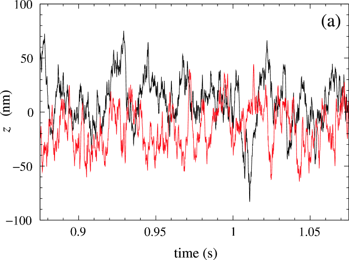
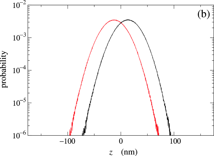
Figure 1: (a) The time series of a typical path $z_{t}$ for the trapped Brownian particle in the fluid moving at the speed $u$ for the forward process (upper curve) and $-u$ for the reversed process (lower curve) with $u=4.24\times 10^{-6}$ m/s. (b) Gaussian probability distributions of the forward and backward experiments. The mean value is located at $\pm u\tau_{R}=\pm 12.9$ nm.

In order to test experimentally that entropy production is related to the time asymmetry of dynamical randomness according to Eq. (30), time series have been recorded for several values of $|u|$. For each value, a pair of time series is generated, one corresponding to the forward process and the other to the reversed process, having first discarded the transient evolution. The time series contain up to $2\times 10^{7}$ points each. Figure 1a depicts examples of paths $z_{t}$ for the trapped Brownian particle in the moving fluid. Figure 1b shows the corresponding stationary distributions for the two time series. They are Gaussian distributions shifted according to Eq. (4).

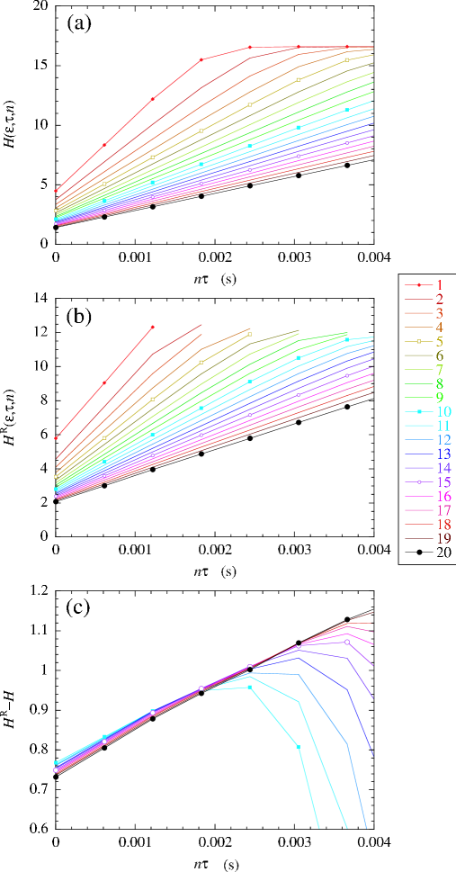
Figure 2: (a) The block entropy (or mean pattern entropy) as a function of time $n\tau$ for the trapped Brownian particle in the fluid moving at the speed $u=4.24\times 10^{-6}$ m/s. The time interval $\tau$ is equal to the sampling time $\tau=1/f=1/8192$ s. The different curves correspond to different values of $\varepsilon=k\times 0.558\ {\rm nm}$ with $k=1,\ldots,20$ given in the right-hand column. The distance used in this calculation is defined by taking the maximum among the distances $|Z(t)-Z_{m}(t)|$ for the times $t=0,\tau,\ldots,(n-1)\tau$. The larger slopes correspond to the smaller value of $\varepsilon$. The linear growth persists up to a maximal value of the mean pattern entropy given by the total length of the time series: $H_{\rm max}=\ln(1.4\times 10^{7})$. (b) The mean reversed block entropy as a function of time corresponding to (a). After a linear growth, $H^{\rm R}$ saturates and falls down to zero (not shown) because of the finiteness of the time series which limits the statistics. (c) Differences between the backward and forward $(\varepsilon,\tau)$ dynamical entropies in (b) and (a) for $\varepsilon$ between $5.6$-$11.2\ {\rm nm}$ for the Brownian particle. Straight lines are fitted to the first part of the curves and their slopes give the entropy production according to Eq. (30).

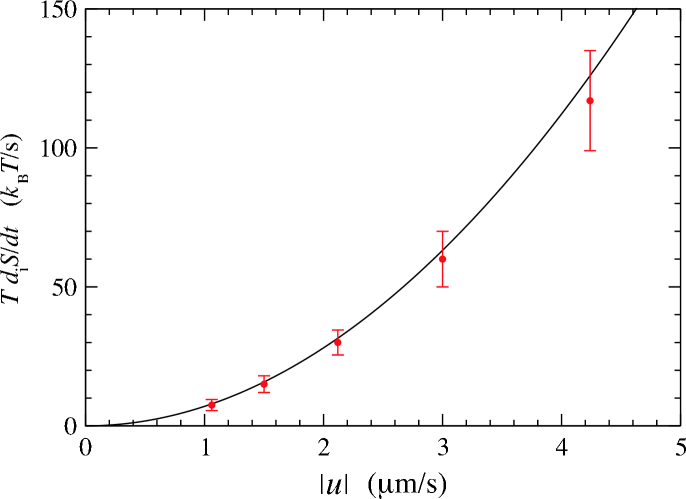
Figure 3: Entropy production of the Brownian particle versus the driving speed $u$. The solid line is the well-known rate of dissipation given by Eq. (9). The dots depict the results of Eq. (30) calculated with the differences between the $(\varepsilon,\tau)$-entropies per unit time. The equilibrium state is at zero speed $u=0$ where the entropy production vanishes.

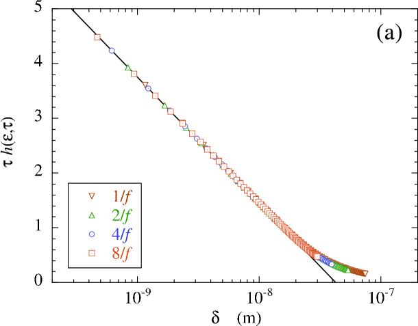
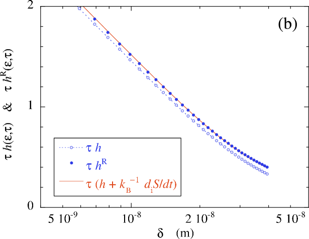
Figure 4: (a) $(\varepsilon,\tau)$-entropy per unit time of the Brownian particle scaled by the time interval $\tau$ as a function of $\delta=\varepsilon/\sqrt{1-\exp(-2\tau/\tau_{R})}$, for different values of the time interval $\tau=1/f,2/f,4/f,8/f$, with the sampling time $1/f=1/8192$ s. The dots are the results of the computation from the time series for the speed $u=4.24\times 10^{-6}$ m/s. The solid line depicts the expected behavior according to Eqs. (27) and (30). (b) Scaled reversed and direct $(\varepsilon,\tau)$-entropies per unit time for $\tau=4/f$. The solid line is the result expected from Eq. (30).

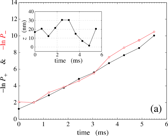
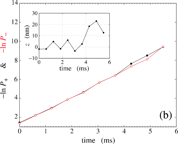
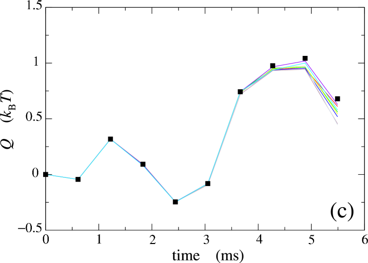
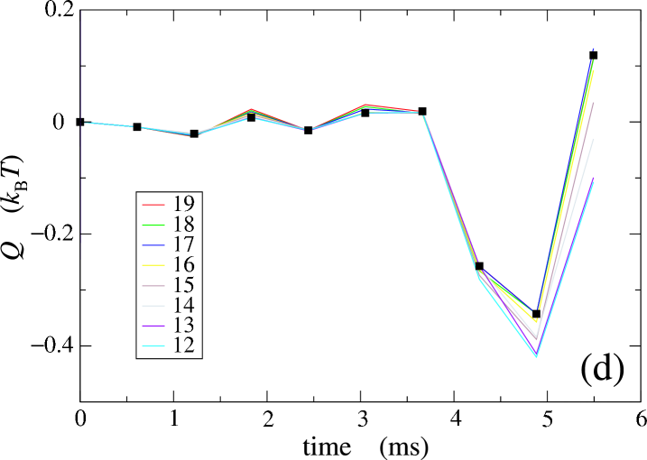
Figure 5: Measure of the heat dissipated by the Brownian particle along two randomly selected trajectories in the time series of Fig. 1. The fluid speeds are $\pm u$ with $u=4.24\times 10^{-6}$ m/s. (a)-(b) Inset: The two randomly selected trajectories. The conditional probabilities $P_{+}$ and $P_{-}$ of the corresponding forward (filled circles) and the backward (open circles) paths for $\varepsilon=8.4\;{\rm nm}$, as evaluated by Eqs. (31) and (32). These probabilities present an exponential decrease modulated by the fluctuations. At time zero, the conditional probabilities are not defined and, instead, we plotted at this time the stationary probabilities for indication. (c)-(d) The dissipated heat given by the logarithm of the ratio of the forward and backward probabilities according to Eq. (14) for different values of $\varepsilon=k\times 0.558\ {\rm nm}$ with $k=12,\ldots,19$ in the range $6.7$-$10.6\;{\rm nm}$. They are compared with the values (squares) directly calculated from Eq. (7). For small values of $\varepsilon$, the agreement is quite good for short time and are within experimental errors for larger time.

The analysis of these time series is performed by calculating the block entropy (20) versus the path duration $n\tau$, and this for different values of $\varepsilon$. Figure 2a shows that the block entropy increases linearly with the path duration $n\tau$ up to a maximum value fixed by the total length of the time series. The time interval is taken equal to the sampling time: $\tau=1/f$. The forward entropy per unit time $h(\varepsilon,\tau)$ is thus evaluated from the linear growth of the block entropy (20) with the time $n\tau$.

Similarly, the time-reversed block entropy (23) is computed using the same reference sequences as for the forward block entropy, reversing each one of them, and getting their probability of occurrence in the backward time series. The resulting time-reversed block entropy is depicted in Fig. 2b versus $n\tau$ for different values of $\varepsilon$. Here also, we observe that $H^{\rm R}$ grows linearly with the time $n\tau$ up to some maximum value due to the lack of statistics over long sequences because the time series is limited. Nevertheless, the linear growth is sufficiently extended that the backward entropy per unit time $h^{\rm R}(\varepsilon,\tau)$ can be obtained from the slopes in Fig. 2b.

Figure 2c depicts the difference between the backward and forward block entropies $H^{\rm R}$ and $H$ versus the time $n\tau$, showing the time asymmetry due to the nonequilibrium constraint. We notice that the differences $H^{\rm R}-H$ are small compared with the block entropies themselves, meaning that dynamical randomness is large although the time asymmetry is small. Accordingly, the values $H^{\rm R}-H$ are more affected by the experimental limitations than the block entropies themselves. In particular, the saturation due to the total length of the time series affects the linearity of $H^{\rm R}-H$ versus $n\tau$. However, we observe the expected independence of the differences $H^{\rm R}-H$ on $\varepsilon$. Indeed, the slope which can be obtained from the differences $H^{\rm R}-H$ versus $n\tau$ cluster around a common value (contrary to what happens for $H$ and $H^{\rm R}$). According to Eq. (30), the slope of $H^{\rm R}-H$ versus $n\tau$ gives the thermodynamic entropy production.

This prediction is indeed verified. Figure 3 compares the difference $h^{\rm R}(\varepsilon,\tau)-h(\varepsilon,\tau)$ with the thermodynamic entropy production given by the rate of dissipation (9) as a function of the speed $u$ of the fluid. We see the good agreement between both, which is the experimental evidence that the thermodynamic entropy production is indeed related to the time asymmetry of dynamical randomness. As expected, the entropy production vanishes at equilibrium where $u=0$.

The dynamical randomness of the Langevin stochastic process can be further analyzed by plotting the scaled entropy per unit time $\tau h(\varepsilon,\tau)$ versus the scaled resolution $\delta\equiv\varepsilon/\sqrt{1-\exp(-2\tau/\tau_{R})}$ for different values of the time interval $\tau$, as depicted in Fig. 4a. According to Eq. (27), the scaled entropy per unit time should behave as $\tau h(\varepsilon,\tau)\simeq\ln(1/\delta)+C$ with some constant $C$ in the limit $\delta\to 0$. Indeed, we verify in Fig. 4a that, in the limit $\delta\to 0$, the scaled curves only depend on the variable $\delta$ with the expected dependence $\ln(1/\delta)$. For large values of $\delta$, the experimental curves deviate from the logarithmic approximation (27), since this latter is only valid for $\delta\to 0$. The calculation in Appendix B shows that we should expect corrections in powers of $\varepsilon^{2}$ to be added to the approximation as $\ln(1/\delta)$.

In Fig. 4b, we depict the scaled direct and reversed $(\varepsilon,\tau)$-entropies per unit time. We compare the behavior of $h^{\rm R}$ with the behavior $\tau h^{\rm R}\simeq\tau\left(h+k_{\rm B}^{-1}d_{\rm i}S/dt\right)$ expected from the formula (30). This figure shows that the direct and reversed $(\varepsilon,\tau)$-entropies per unit time are quantities which are large with respect to their difference due to the nonequilibrium constraint. This means that the positive entropy production is a small effect on the top of a substantial dynamical randomness.

Maxwell’s demon vividly illustrates the paradox that the dissipated heat is always positive at the macroscopic level although it may take both signs if considered at the microscopic level of individual stochastic trajectories. The resolution of Maxwell’s paradox can be remarkably demonstrated with the experimental data. Indeed, the heat dissipated along an individual trajectories is given by Eq. (7) and can be obtained by searching for recurrences in the time series according to Eq. (14). The conditional probabilities entering Eq. (14) are evaluated in terms of the joint probabilities (19) and (22) according to

$$P_{+}({\textbf{\em Z}};\varepsilon,\tau,n|Z_{0}) = P_{+}({\textbf{\em Z}};\varepsilon,\tau,n)/P_{+}(Z_{0};\varepsilon,\tau,1)$$ (31)

$$P_{-}({\textbf{\em Z}}^{\rm R};\varepsilon,\tau,n|Z_{n-1}) = P_{-}({\textbf{\em Z}}^{\rm R};\varepsilon,\tau,n)/P_{-}(Z_{n-1};\varepsilon,\tau,1)$$ (32)

where we notice that the probabilities with $n=1$ are approximately equal to the corresponding stationary probability density (4) multiplied by the range $dz=2\varepsilon$. The heat dissipated along two randomly selected paths are plotted in Fig. 5. We see the very good agreement between the values computed with Eq. (7) using each path and Eq. (14) using the probabilities of recurrences in the time series. We observe that, at the level of individual trajectories, the heat exchanged between the particle and the surrounding fluid can be positive or negative because of the molecular fluctuations. It is only by averaging over the forward process that the dissipated heat takes the positive value depicted in Fig. 3. Indeed, Fig. 3 is obtained after averaging over many reference paths as those of Fig. 5. The positivity of the thermodynamic entropy production results from this averaging, which solves Maxwell’s paradox.

V Electric noise in $RC$ circuits

The second system we have investigated is an $RC$ electric circuit driven out of equilibrium by a current source which imposes the mean current $I$ GC04 . The current fluctuates in the resistor because of the intrinsic Nyquist thermal noise ZCC04 . The $RC$ electric circuit and the dragged Brownian particle, although physically different, are known to be formally equivalent by the correspondence given in Table 1.

The electric circuit is composed of a capacitor with capacitance $C=278\;\rm{pF}$ in parallel with a resistor of resistance $R=9.22\ {\rm M}\Omega$. The relaxation time of the circuit is $\tau_{R}=RC=2.56\times 10^{-3}\;\rm{s}$. The charge $q_{t}$ going through the resistor during the time interval $t$ is acquired at the sampling frequency $f=8192\;{\rm Hz}$. The temperature is here also equal to $T=298\;{\rm K}$.

The mean square charge of the Nyquist thermal fluctuations is $\sigma=\sqrt{k_{\rm B}TC}=6.7\times 10^{3}\,e$ where $e=1.602\times 10^{-19}$ C is the electron charge. The diffusion coefficient is $D=\sigma^{2}/\tau_{R}=1.75\times 10^{10}\;e^{2}/{\rm s}$. The ratio of the relaxation time to the sampling time is here equal to $f\tau_{R}=21$.

As for the first system, pairs of time series for opposite drivings $\pm I$ are recorded. Their length are $2\times 10^{7}$ points each. Figure 6 depicts an example of a pair of such paths with the corresponding probability distribution of the charge fluctuations.

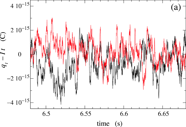
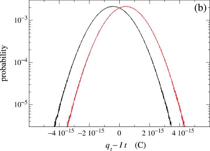
Figure 6: (a) The time series of a typical path $q_{t}-It$ for the Nyquist noise in the $RC$ electric circuit driven by the current $I$ (upper curve) and opposite current $-I$ (lower curve) with $I=1.67\times 10^{-13}$ A. (b) Gaussian probability distributions of the forward and backward experiments. The unit of the electric charge $q_{t}-It$ is the Coulomb (C).

The block entropies are here also calculated using Eqs. (20) and (23) and the $(\varepsilon,\tau)$-entropies per unit time are obtained from their linear growth as a function of the time $n\tau$. The scaled entropies per unit time $\tau h$ are depicted versus $\delta$ in Fig. 7a. Here again, the scaled entropy per unit time is verified to depend only on $\delta$ for $\delta\to 0$, as expected from the analytical calculation in Appendix B. In Fig. 7b, we compare the scaled reversed $(\varepsilon,\tau)$-entropy per unit time to the behavior $\tau h^{R}\simeq\tau\left(h+k_{\rm B}^{-1}d_{\rm i}S/dt\right)$, expected by our central result (30).

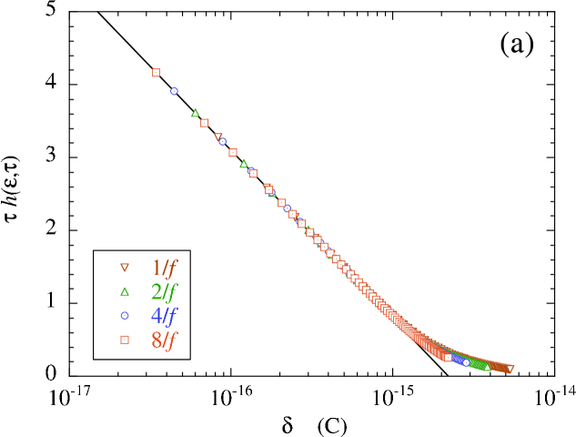
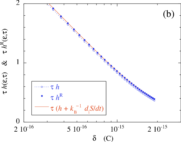
Figure 7: (a) $(\varepsilon,\tau)$-entropy per unit time of the $RC$ electric circuit scaled by the time interval $\tau$ as a function of $\delta=\varepsilon/\sqrt{1-\exp(-2\tau/\tau_{R})}$, for different values of the time interval $\tau=1/f,2/f,4/f,8/f$, with the sampling time $1/f=1/8192$ s. The dots are the results of the computation from the time series for the current $I=1.67\times 10^{-13}$ A. The solid line depicts the expected behavior according to Eqs. (27) and (30). (b) Scaled reversed and direct $(\varepsilon,\tau)$-entropies per unit time for $\tau=4/f$. The solid line is the result expected from Eq. (30). The unit of $\delta$ is the Coulomb (C).

The difference between the time-reversed and direct $(\varepsilon,\tau)$-entropies per unit time is then compared with the dissipation rate expected with Joule’s law. We observe the nice agreement between both in Fig. 8, which confirms the validity of Eq. (30). Here also, we observe that the entropy production vanishes with the current at equilibrium.

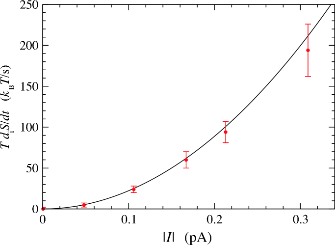
Figure 8: Entropy production of the $RC$ electric circuit versus the injected current $I$. The solid line is the Joule law, $Td_{\rm i}S/dt=RI^{2}$. The dots are the results of Eq. (30). The equilibrium state is at zero current, $I=0$, where the entropy production is observed to vanish.

VI Discussion

In this section, we discuss about the comparison between the present results and other nonequilibrium relations.

The relation (30) expresses the entropy production as the difference between the backward and forward $(\varepsilon,\tau)$-entropies per unit time. The backward process is obtained by reversing the driving constraints, which is also a characteristic feature of Crooks relation C99 . However, Crooks relation is concerned with systems driven by time-dependent external controls starting at equilibrium. In constrast, our results apply to nonequilibrium steady states. Another point is that Crooks relation deals with the fluctuations of the work performed on the system, while the present relation (30) gives the mean value of the entropy production and, this, in terms of path probabilities. In this respect, the relation (30) is closer to a formula recently obtained for the mean value of the dissipated work in systems driven out of equilibrium by time-dependent external controls KPV07 . This formula relates the mean value of the dissipated work to the logarithm of the ratio between two phase-space probability densities associated with the forward and backward processes, respectively. These phase-space probability densities could in principle be expressed as path probabilities. Nevertheless, these latter would be defined for systems driven over a finite time interval starting from the equilibrium state, although the present equation (30) applies to nonequilibrium steady states reached in the long-time limit.

We now compare our results to the extended fluctuation theorem, which concerns nonequilibrium steady states ZC03 ; ZCC04 ; GC04 . The extended fluctuation theorem is a symmetry relation of the large-deviation properties of the fluctuating heat dissipation (7) during a time interval $t$. The probability that this fluctuating quantity takes the value

$$\zeta\simeq\frac{1}{t}\frac{Q_{t}}{T}$$ (33)

decays exponentially with the rate

$$G(\zeta)\equiv\lim_{t\to\infty}-\frac{1}{t}\ln{\rm Pr}\left\{\zeta<\frac{Q_{t}}{tT}<\zeta+d\zeta\right\}$$ (34)

This rate is a function of the value $\zeta$. Since the variable $\zeta$ can significantly deviate from the statistical average for some large fluctuations, the rate (34) is called a large-deviation function. The extended fluctuation theorem states that the ratio of the probability of a positive fluctuation to the probability of a negative one increases exponentially as $\exp(\zeta t)$ in the long-time limit $t\to\infty$ and over a range of values of $\zeta$, which is limited by its average $\langle\zeta\rangle$ ZC03 ; ZCC04 ; GC04 . Taking the logarithm of the ratio and the long-time limit, the extended fluctuation theorem can therefore be expressed as the following symmetry relation for the decay rate (34):

$$\zeta=k_{\rm B}\Big{[}G(-\zeta)-G(\zeta)\Big{]}\qquad\mbox{for}\quad-\langle\zeta\rangle\leq\zeta\leq\langle\zeta\rangle$$ (35)

In this form, we notice the analogy with Eq. (30). A priori, the decay rate (34) can be compared with the $(\varepsilon,\tau)$-entropy per unit time, which is also a decay rate. However, the decay rate (34) concerns the probability of all the paths with dissipation $\zeta$ while the $(\varepsilon,\tau)$-entropy per unit time concerns the probability of the paths within a distance $\varepsilon$ of some reference typical paths. The $(\varepsilon,\tau)$-entropy per unit time is therefore probing more deeply into the fluctuations down to the microscopic dynamics. In principle, this latter should be reached by zooming to the limit $\varepsilon\to 0$.

A closer comparison can be performed by considering the mean value of the fluctuating quantity $\zeta$ which gives the thermodynamic entropy production:

$$\langle\zeta\rangle=\lim_{t\to\infty}\frac{1}{t}\frac{\langle Q_{t}\rangle}{T}=\frac{d_{\rm i}S}{dt}$$ (36)

Since the decay rate (34) vanishes at the mean value:

$$G\big{(}\langle\zeta\rangle\big{)}=0$$ (37)

we obtain the formula

$$\langle\zeta\rangle=k_{\rm B}G\big{(}-\langle\zeta\rangle\big{)}$$ (38)

which can be quantitatively compared with Eq. (30) since both give the thermodynamic entropy production. Although the time-reversed entropy per unit time $h^{\rm R}(\varepsilon,\tau)$ is a priori comparable with the decay rate $G(-\zeta)$, it turns out that they are different and satisfy in general the inequality $h^{\rm R}(\varepsilon,\tau)\geq G(-\langle\zeta\rangle)$ since the entropy per unit time is always non negative $h(\varepsilon,\tau)\geq 0$. Moreover, $h(\varepsilon,\tau)$ is typically a large positive quantity. The greater the dynamical randomness, the larger the entropy per unit time $h(\varepsilon,\tau)$, as expected in the limit where $\varepsilon$ goes to zero. This shows that the $(\varepsilon,\tau)$-entropy per unit time probes finer scales in the path space where the time asymmetry is tested.

VII Conclusions

We have here presented detailed experimental results giving evidence that the thermodynamic entropy production finds its orgin in the time asymmetry of dynamical randomness in the nonequilibrium fluctuations of two experimental systems. The first is a Brownian particle trapped by an optical tweezer in a fluid moving at constant speed $0\leq|u|<4.3\;\mu$m/s. The second is the electric noise in an $RC$ circuit driven by a constant source of current $0\leq|I|<0.3$ pA. In both systems, long time series are recorded, allowing us to carry out the statistical analysis of their properties of dynamical randomness.

The dynamical randomness of the fluctuations is characterized in terms of $(\varepsilon,\tau)$-entropies per unit time, one for the forward process and the other for the reversed process with opposite driving. These entropies per unit time measure the temporal disorder in the time series. The fact that the stochastic processes is continuous implies that the entropies per unit time depend on the resolution $\varepsilon$ and the sampling time $\tau$. The temporal disorder of the forward process is thus characterized by the entropy per unit time $h(\varepsilon,\tau)$, which is the mean decay rate of the path probabilities. On the other hand, the time asymmetry of the process can be tested by evaluating the amount of time-reversed paths of the forward process among the paths of the reversed process. This amount is evaluated by the probabilities of the time-reversed forward paths in the reversed process and its mean decay rate, which defines the time-reversed entropy per unit time $h^{\rm R}(\varepsilon,\tau)$. The time asymmetry in the process can be measured by the difference $h^{\rm R}(\varepsilon,\tau)-h(\varepsilon,\tau)$. At equilibrium where detailed balance holds, we expect that the probability distribution ruling the time evolution is symmetric under time reversal so that this difference should vanish. In contrast, out of equilibrium, detailed balance is no longer satisfied and we expect that the breaking of the time-reversal symmetry for the invariant probability distribution of the nonequilibrium steady state. In this case, a non-vanishing difference is expected.

The analysis of the experimental data shows that the difference of $(\varepsilon,\tau)$-entropies per unit time is indeed non vanishing. Moreover, we have the remarkable result that the difference gives the thermodynamic entropy production. The agreement between the difference and the thermodynamic entropy production is obtained for the driven Brownian motion up to an entropy production of nearly $120\,k_{\rm B}T/{\rm s}$. For electric noise in the $RC$ circuit, the agreement is obtained up to an entropy production of nearly $200\,k_{\rm B}T/{\rm s}$. These results provide strong evidence that the thermodynamic entropy production arises from the breaking of time-reversal symmetry of the dynamical randomness in out-of-equilibrium systems.

Acknowledgments. This research is financially supported by the F.R.S.-FNRS Belgium, the “Communauté française de Belgique” (contract “Actions de Recherche Concertées” No. 04/09-312), and by the French contract ANR-05-BLAN-0105-01.

Appendix A Path probabilities and dissipated heat

The detailed derivation of Eq. (14) is here presented for the case of the Langevin stochastic process ruled by Eq. (1). This stochastic process is Markovian and described by a Green function $G(z,z_{0};t)$ which is the conditional probability that the particle moves to the position $z$ during the time interval $t$ given that its initial position was $z_{0}$ C43 . For small values $\tau$ of the time interval, this Green function reads

$$G(z,z_{0};\tau)\simeq\sqrt{\frac{\beta\alpha}{4\pi\tau}}\,\exp\left\{-\frac{\beta\alpha}{4\tau}\left[z-z_{0}-\tau\left(\frac{F(z_{0})}{\alpha}+u\right)\right]^{2}\right\}$$ (39)

If we discretize the time axis into small time intervals $\tau$, the path probability (12) becomes

$$P[z_{t}|z_{0}]\propto\prod_{i=1}^{n-1}G(z_{i},z_{i-1};\tau)$$ (40)

with $(n-1)\tau=t$. The ratio (14) of the direct and reversed path probabilities is thus given by

$$\frac{P_{+}[z_{t}|z_{0}]}{P_{-}[z_{t}^{\rm R}|z_{0}^{\rm R}]}\simeq\prod_{i=1}^{n-1}\frac{G_{+}(z_{i},z_{i-1};\tau)}{G_{-}(z_{n-i-1},z_{n-i};\tau)}$$ (41)

where the subscript is the sign of the fluid speed $u$. Inserting the expression (39) for the Green functions, we get

$$\ln\frac{P_{+}[z_{t}|z_{0}]}{P_{-}[z_{t}^{\rm R}|z_{0}^{\rm R}]} \simeq -\frac{\beta\alpha}{4\tau}\sum_{i=1}^{n-1}\left\{\left[z_{i}-z_{i-1}-\tau\left(\frac{F(z_{i-1})}{\alpha}+u\right)\right]^{2}-\left[z_{n-i-1}-z_{n-i}-\tau\left(\frac{F(z_{n-i})}{\alpha}-u\right)\right]^{2}\right\}$$ (42)

$$= \frac{\beta}{2}\sum_{i=1}^{n-1}\left[(z_{i}-z_{i-1})F(z_{i-1})-(z_{n-i-1}-z_{n-i})F(z_{n-i})\right]-\frac{\beta u\tau}{2}\sum_{i=1}^{n-1}\left[F(z_{i-1})+F(z_{n-i})\right]+O(\tau)$$

$$= \beta\sum_{i=1}^{n-1}\frac{F(z_{i-1})+F(z_{i})}{2}(z_{i}-z_{i-1})-\beta u\tau\sum_{i=1}^{n-1}\frac{F(z_{i-1})+F(z_{i})}{2}+O(\tau)$$

where we used the substitution $n-i\to i$ in the last terms of each sum. In the continuous limit $n\rightarrow\infty$, $\tau\rightarrow 0$ with $(n-1)\tau=t$, the sums become integrals and we find

$$\ln\frac{P_{+}[z_{t}|z_{0}]}{P_{-}[z_{t}^{\rm R}|z_{0}^{\rm R}]} = \beta\left[\int_{z_{0}}^{z_{t}}F(z)\,dz-u\int_{0}^{t}F(z_{t^{\prime}})\,dt^{\prime}\right]$$ (43)

$$= \beta\left[V(z_{0})-V(z_{t})-u\int_{0}^{t}F(z_{t^{\prime}})\,dt^{\prime}\right]$$

since $F(z)=-\partial_{z}V(z)$. We thus obtain the expression given in Eq. (14).

Now, we show that the detailed balance condition

$$\mbox{equilibrium:}\qquad P_{+}[z_{t}]=P_{-}[z_{t}^{\rm R}]\qquad(u=0)$$ (44)

holds in the equilibrium state when the speed of the fluid is set to zero. Indeed, the equilibrium probability density of a Brownian particle in a potential $V(z)$ is given by

$$p_{\rm eq}(z)=C\,\exp\left[-\beta V(z)\right]$$ (45)

with a normalization constant $C$. Since the joint probabilities are related to the conditional ones by Eq. (13) with $p_{\rm st}=p_{\rm eq}$ at equilibrium, we find

$$\ln\frac{P_{+}[z_{t}]}{P_{-}[z_{t}^{\rm R}]}\Big{|}_{\rm eq}=\ln\frac{P_{+}[z_{t}|z_{0}]\,p_{\rm eq}(z_{0})}{P_{-}[z_{t}^{\rm R}|z_{0}^{\rm R}]\,p_{\rm eq}(z_{0}^{\rm R})}\Big{|}_{\rm eq}=0$$ (46)

The vanishing occurs at zero speed $u=0$ as a consequence of Eqs. (43), (45), and $z_{0}^{\rm R}=z_{t}$. Hence, the detailed balance condition is satisfied at equilibrium. Therefore, the last expression of Eq. (15) vanishes at equilibrium with the entropy production, as expected.

Appendix B Dynamical randomness of the Langevin stochastic process

In this appendix, we evaluate the $(\varepsilon,\tau)$-entropy per unit time of the Grassberger-Procaccia algorithm for the Langevin stochastic process of Eq. (1) with a harmonic trap potential. In this case, the Langevin process is an Ornstein-Uhlenbeck stochastic process for the new variable

$$y\equiv z-u\tau_{R}$$ (47)

The Langevin equation of this process is

$$\frac{dy}{dt}=-\frac{y}{\tau_{R}}+\frac{\xi_{t}}{\alpha}$$ (48)

The probability density that the continuous random variable $Y(t)$ takes the values ${\bf y}=(y_{0},y_{1},...,y_{n-1})$ at the successive times $0,\tau,2\tau,...,(n-1)\tau$ factorizes since the random process is Markovian:

$$p(y_{0},...,y_{n-1})=G(y_{n-1},y_{n-2};\tau)\cdots G(y_{1},y_{0};\tau)\,p_{\rm st}(y_{0})$$ (49)

with the Green function

$$G(y,y_{0};t)=\frac{1}{\sqrt{2\pi\sigma^{2}(1-{\rm e}^{-2t/\tau_{R}})}}\exp\left[-\frac{(y-{\rm e}^{-t/\tau_{R}}y_{0})^{2}}{2\sigma^{2}(1-{\rm e}^{-2t/\tau_{R}})}\right]$$ (50)

with the variance

$$\sigma^{2}=\frac{k_{\rm B}T}{k}$$ (51)

The stationary probability density is given by the Gaussian distribution

$$p_{\rm st}(y)=\lim_{t\to\infty}G(y,y_{0};t)=\frac{1}{\sqrt{2\pi\sigma^{2}}}\exp\left(-\frac{y^{2}}{2\sigma^{2}}\right)$$ (52)

Denoting by ${\bf y}^{\rm T}$ the transpose of the vector $\bf y$, the joint probability density (49) can be written as the multivariate Gaussian distribution

$$p(y_{0},...,y_{n-1})=\frac{\exp\left(-\frac{1}{2}{\bf y}^{\rm T}\cdot{\bf C}_{n}^{-1}\cdot{\bf y}\right)}{(2\pi)^{\frac{n}{2}}(\det{\bf C}_{n})^{\frac{1}{2}}}$$ (53)

in terms of the correlation matrix

$${\bf C}_{n}=\sigma^{2}\left(\begin{array}[]{ccccc}1&r&r^{2}&\ldots&r^{n-1}\\ r&1&r&\ldots&r^{n-2}\\ r^{2}&r&1&\ldots&r^{n-3}\\ \vdots&\vdots&\vdots&\ddots&\vdots\\ r^{n-1}&r^{n-2}&r^{n-3}&\ldots&1\\ \end{array}\right)$$ (59)

with

$$r=\exp(-\tau/\tau_{R})$$ (60)

The inverse of the correlation matrix is given by

$${\bf C}^{-1}_{n}=\frac{\sigma^{-2}}{(1-r^{2})}\left(\begin{array}[]{cccccc}1&-r&0&\ldots&0&0\\ -r&1+r^{2}&-r&\ldots&0&0\\ 0&-r&1+r^{2}&&0&0\\ \vdots&\vdots&\vdots&\ddots&\vdots&\vdots\\ 0&0&0&\ldots&1+r^{2}&-r\\ 0&0&0&\ldots&-r&1\\ \end{array}\right)$$ (67)

and its determinant by

$$\det{\bf C}_{n}=\sigma^{2n}(1-r^{2})^{n-1}$$ (68)

The $(\varepsilon,\tau)$-entropy per unit time is defined by

$$h(\varepsilon,\tau)=\lim_{n\rightarrow\infty}-\frac{1}{n\tau}\int_{-\infty}^{+\infty}dy_{0}\cdots\int_{-\infty}^{+\infty}dy_{n-1}\;p(y_{0},...,y_{n-1})\ln\int_{-\varepsilon}^{+\varepsilon}d\eta_{0}\cdots\int_{-\varepsilon}^{+\varepsilon}d\eta_{n-1}\;p(y_{0}+\eta_{0},...,y_{n-1}+\eta_{n-1})$$ (69)

where $\{y_{j}^{\prime}=y_{j}+\eta_{j}\}_{j=0}^{n-1}$ represents the tube of trajectories satisfying the conditions $|y_{j}^{\prime}-y_{j}|<\varepsilon$ with $j=0,1,...,n-1$, around the reference trajectory sampled at the successive positions $\{y_{j}\}_{j=0}^{n-1}$. After expanding in powers of the variables $\eta_{j}$ and evaluating the integrals over $-\varepsilon<\eta_{j}<+\varepsilon$, the logarithm is obtained as

$$\ln\int_{-\varepsilon}^{+\varepsilon}d\eta_{0}\cdots\int_{-\varepsilon}^{+\varepsilon}d\eta_{n-1}\;p(y_{0}+\eta_{0},...,y_{n-1}+\eta_{n-1})=\ln\frac{(2\varepsilon)^{n}}{(2\pi)^{\frac{n}{2}}(\det{\bf C}_{n})^{\frac{1}{2}}}-\frac{1}{2}\,{\bf y}^{\rm T}\cdot{\bf C}_{n}^{-1}\cdot{\bf y}+O(\varepsilon^{2})$$ (70)

The integrals over $-\infty<y_{j}<+\infty$ can now be calculated to get the result (27) by using Eq. (68). We find

$$h(\varepsilon,\tau)=\frac{1}{\tau}\ln\sqrt{\frac{\pi{\rm e}\sigma^{2}}{2\varepsilon^{2}}(1-r^{2})}+O(\varepsilon^{2})$$ (71)

Since the relaxation time is given by Eq. (5) and the diffusion coefficient by Eq. (28), the variance of the fluctuations can be rewritten as $\sigma^{2}=k_{\rm B}T/k=D\tau_{R}$. Substituting in Eq. (71), we obtain the $(\varepsilon,\tau)$-entropy per unit time given by Eq. (27). The above calculation shows that the $(\varepsilon,\tau)$-entropy per unit time of the Ornstein-Uhlenbeck process is of the form

$$h(\varepsilon,\tau)=\frac{1}{\tau}\;\phi\left(\frac{D\tau_{R}}{\varepsilon^{2}},{\rm e}^{-\tau/\tau_{R}}\right)$$ (72)

with some function $\phi(s,r)$ of $s=D\tau_{R}/\varepsilon^{2}=\sigma^{2}/\varepsilon^{2}$ and $r=\exp(-\tau/\tau_{R})$.

In the limit where the time interval $\tau$ is much smaller than the relaxation time $\tau_{R}$, the only dimensionless variable is the combination $D\tau/\varepsilon^{2}$. In this case, we recover the result that the $(\varepsilon,\tau)$-entropy per unit time is given by

$$h(\varepsilon,\tau)=\frac{1}{\tau}\;\psi\left(\frac{2D\tau}{\varepsilon^{2}}\right)\qquad\mbox{for}\quad\tau\ll\tau_{R}$$ (73)

This $(\varepsilon,\tau)$-entropy per unit time is characteristic of pure diffusion without trap potential, as previously shown GW93 ; G98 ; GBFSGDC98 ; BSFGGDC01 .

References

- (1) D. Andrieux, P. Gaspard, S. Ciliberto, N. Garnier, S. Joubaud, and A. Petrosyan, Phys. Rev. Lett. 98, 150601 (2007).
- (2) P. Gaspard and X. J. Wang, Phys. Rep. 235, 291 (1993).
- (3) J.-P. Eckmann and D. Ruelle, Rev. Mod. Phys. 57, 617 (1985).
- (4) P. Gaspard and G. Nicolis, Phys. Rev. Lett. 65, 1693 (1990).
- (5) J. R. Dorfman and P. Gaspard, Phys. Rev. E 51, 28 (1995).
- (6) P. Gaspard, I. Claus, T. Gilbert, and J. R. Dorfman, Phys. Rev. Lett. 86, 1506 (2001).
- (7) D. J. Evans, E. G. D. Cohen, and G. P. Morriss, Phys. Rev. Lett. 71, 2401 (1993).
- (8) D. J. Evans and D. J. Searles, Phys. Rev. E 50, 1645 (1994).
- (9) G. Gallavotti and E. G. D. Cohen, Phys. Rev. Lett. 74, 2694 (1995).
- (10) J. Kurchan, J. Phys. A: Math. Gen. 31, 3719 (1998).
- (11) J. L. Lebowitz and H. Spohn, J. Stat. Phys. 95, 333 (1999).
- (12) C. Maes, J. Stat. Phys. 95, 367 (1999).
- (13) C. Maes and K. Netočný, J. Stat. Phys. 110, 269 (2003).
- (14) G. M. Wang, E. M. Sevick, E. Mittag, D. J. Searles, and D. J. Evans, Phys. Rev. Lett. 89, 050601 (2002).
- (15) R. van Zon and E. G. D. Cohen, Phys. Rev. Lett. 91, 110601 (2003).
- (16) R. van Zon, S. Ciliberto and E. G. D. Cohen, Phys. Rev. Lett. 92, 130601 (2004).
- (17) N. Garnier and S. Ciliberto, Phys. Rev. E 71, R060101 (2005).
- (18) F. Douarche, S. Joubaud, N. B. Garnier, A. Petrosyan, and S. Ciliberto, Phys. Rev. Lett. 97, 140603 (2006).
- (19) S. Schuler, T. Speck, C. Tietz, J. Wrachtrup, and U. Seifert, Phys. Rev. Lett. 94, 180602 (2005).
- (20) U. Seifert, Phys. Rev. Lett. 95, 040602 (2005).
- (21) T. Taniguchi and E. G. D. Cohen, J. Stat. Phys. 126, 1 (2006).
- (22) R. J. Harris and G. M. Schütz, J. Stat. Mech. P07020 (2007).
- (23) D. Andrieux and P. Gaspard, J. Stat. Phys. 127, 107 (2007).
- (24) D. Andrieux and P. Gaspard, J. Stat. Mech. P02006 (2007).
- (25) G. E. Crooks, Phys. Rev. E 60, 2721 (1999).
- (26) F. Douarche, S. Ciliberto, and A. Petrosyan, J. Stat. Mech. P09011 (2005).
- (27) D. Collin, F. Ritort, C. Jarzynski, S. B. Smith, I. Tinoco Jr., and C. Bustamante, Nature 437, 231 (2005).
- (28) C. Jarzynski, Phys. Rev. E 73, 046105 (2006).
- (29) R. Kawai, J. M. R. Parrondo, and C. Van den Broeck, Phys. Rev. Lett. 98, 080602 (2007).
- (30) P. Gaspard, New J. Phys. 7, 77 (2005).
- (31) P. Gaspard, Physica A 369, 201 (2006).
- (32) B. Derrida, P. Gaspard, and C. Van den Broeck, Editors, Work, dissipation, and fluctuations in nonequilibrium physics, special issue of C. R. Physique (2007).
- (33) P. Gaspard, J. Stat. Phys. 117, 599 (2004).
- (34) V. Lecomte, C. Appert-Rolland, and F. van Wijland, Phys. Rev. Lett. 95, 010601 (2005).
- (35) J. Naudts and E. Van der Straeten, Phys. Rev. E 74, 040103R (2006).
- (36) A. Porporato, J. R. Rigby, and E. Daly, Phys. Rev. Lett. 98, 094101 (2007).
- (37) K. Sekimoto, J. Phys. Soc. Japan 66, 1234 (1997).
- (38) L. Onsager and S. Machlup, Phys. Rev. 91, 1505 (1953).
- (39) S. Kullback and R. A. Leibler, Ann. Math. Stat. 22, 79 (1951).
- (40) A. Wehrl, Rev. Mod. Phys. 50, 221 (1978).
- (41) C. Shannon, Bell System Tech. J. 27, 379, 623 (1948).
- (42) A. Kolmogorov, IEEE Trans. Inform. Theory 2, 102 (1956).
- (43) T. Berger, Rate Distortion Theory (Englewood Cliffs, Prentice Hall, 1971).
- (44) P. Grassberger and I. Procaccia, Phys. Rev. A 28, 2591 (1983).
- (45) A. Cohen and I. Procaccia, Phys. Rev. A 31, 1872 (1985).
- (46) P. Gaspard, Chaos, Scattering, and Statistical Mechanics (Cambridge University Press, Cambridge UK, 1998).
- (47) P. Gaspard, M. E. Briggs, M. K. Francis, J. V. Sengers, R. W. Gammon, J. R. Dorfman, and R. V. Calabrese, Nature 394, 865 (1998).
- (48) M. E. Briggs, J. V. Sengers, M. K. Francis, P. Gaspard, R. W. Gammon, J. R. Dorfman, and R. V. Calabrese, Physica A 296, 42 (2001).
- (49) P. Billingsley, Ergodic Theory and Information (Wiley, New York, 1965).
- (50) B. Schnurr, F. Gittes, F. C. MacKintosh, and C. F. Schmidt, Macromolecules 30(25), 7781 (1997).
- (51) In Ref. AGCGJP07 , the same experiment was described in the frame of coordinate where the fluid is at rest and the trap is moving.
- (52) S. Chandrasekhar, Rev. Mod. Phys. 15, 1 (1943).