Boundary of central tiles associated with Pisot beta-numeration and purely periodic expansions

Abstract.

This paper studies tilings related to the $\beta$-transformation when $\beta$ is a Pisot number (that is not supposed to be a unit). Then it applies the obtained results to study the set of rational numbers having a purely periodic $\beta$-expansion. Secial focus is given to some quadratic examples.

1. Introduction

Beta-numeration generalises usual binary and decimal numeration. Taking any real number $\beta>1$, it consists in expanding numbers $x\in[0,1]$ as power series in base $\beta^{-1}$ with digits in $\mathcal{D}=\{0,\dots,\lceil\beta\rceil-1\}$. As for $\beta\in\mathbb{N}$, the digits are obtained with the so-called greedy algorithm: the $\beta$-transformation $T_{\beta}:\ x\mapsto\beta x\pmod{1}$ computes the digits $u_{i}=\lfloor\beta T_{\beta}^{i-1}(x)\rfloor$, which yield the expansion $x=\sum_{i\geq 1}u_{i}\beta^{-i}$. The sequence of digits is denoted by $d_{\beta}(x)=(u_{i})_{i\geq 1}$.

The set of expansions $(u_{i})_{i\geq 1}$ has been characterised by Parry in [Par60]) (see Theorem 2.1 below). In case $\beta$ is a Pisot number, Bertrand [Ber77] and Schmidt [Sch80] proved independently that the $\beta$-expansion $d_{\beta}(x)$ of a real number $x\in[0,1]$ is ultimately periodic if and only if $x$ belongs to $\mathbb{Q}(\beta)\cap[0,1]$. A further natural question was to identify the set of numbers with purely periodic expansions. For $\beta\in{\mathbb{N}}$, it is known for a long time that rational numbers $a/b$ with purely periodic $\beta$-expansion are exactly those such that $b$ and $\beta$ are coprime, the length of the period being the order of $\beta$ in $({\mathbb{Z}}/b{\mathbb{Z}})^{*}$. Using an approximation and renormalisation technique, Schmidt proved in [Sch80] that when $\beta^{2}=n\beta+1$ and $n\in{\mathbb{N}}^{*}$, then all rational numbers less than 1 have a purely periodic $\beta$-expansion. This result was completed in [HI97], to $\beta^{2}=n\beta-1$, $n\geq 3$, with respect to which no rational number has purely periodic $\beta$-expansion. More generally, the latter result is satisfied by all $\beta$’s admitting at least one positive real Galois conjugate in $[0,1]$ [Aki98][Proposition 5]. Ito and Rao characterised the real numbers having purely periodic $\beta$-expansion in terms of the associated Rauzy fractal for any Pisot unit $\beta$ [IR04], whereas the non-unit case has been handled in [BS07]. The length of the periodic expansions with respect to quadratic Pisot units were investigated in [QRY05].

Another natural question is to determinate the real numbers with finite expansion. According to [FS92], we say that $\beta$ satisfies the finiteness property (F) if the positive elements of $\mathbb{Z}[1/\beta]$ all have a finite $\beta$-expansion (the converse is clear). A complete characterisation of $\beta$ satisfying the finiteness property (F) is known when $\beta$ is a Pisot number of degree 2 or 3 [Aki00]. It turns out that those numbers $\beta$ also play a role in the question of purely periodic expansions. Indeed, if $\beta$ is a unit Pisot number and satisfies the finiteness property (F), then there exists a neighbourhood of 0 in $\mathbb{Q}_{+}$ whose elements all have purely periodic $\beta$-expansion [Aki98]. This result is quite unexpected since there is no reason a priori for obtaining only purely periodic expansion around zero.

The present paper investigates the case when $\beta$ is still a Pisot number, but not necessarily a unit. We make use of the connection between pure periodicity and a compact self-similar representation of numbers having no fractional part in their $\beta$-expansion, similarly as in [IR04, BS07]. This representation is called the central tile associated with $\beta$ (Rauzy fractal, or atomic surface may also be encountered in the literature, see e.g. the survey [BS05]). For elements $x$ of the ring ${\mathbb{Z}}[1/\beta]$, so-called $x$-tiles are introduced, so that the central tile is a finite union of $x$-tiles up to translation. Those $x$-tiles provide a covering of the space we are working in. We first discuss the topological and metric properties of the central tile in the flavor of [Aki02, Pra99, Sie03] and the relations between the tiles.

In the unit case, the covering by $x$-tiles is defined in a Euclidean space ${\mathbb{K}}_{\infty}\simeq{\mathbb{R}}^{r-1}\times{\mathbb{C}}^{s}$, where $d=r+2s$ is the degree of the extension $[{\mathbb{Q}}(\beta):{\mathbb{Q}}]$ and $r$ the number of real roots of beta’s minimal polynomial. The space ${\mathbb{K}}_{\infty}$ can be interpreted as the product of all Archimedean completions of ${\mathbb{Q}}(\beta)$ distinct from the usual one. It turns out that this is not enough in general: in order to have suitable measure-preserving properties, one has to take into account the non-Archimedean completions associated with the principal ideal $(\beta)$. Therefore, everything takes place in the product ${\mathbb{K}}_{\beta}={\mathbb{K}}_{\infty}\times{\mathbb{K}}_{f}$, where the latter is a finite product of local fields. In the framework of substitutions, this approach has been already used in [Sie03], and was inspired by [Rau88]. See also [Sin06]. Completions and (complete) tiles are introduced in Section 3. We discuss why taking into account non-Archimedean completions is suitable from a tiling point of view: when the finiteness property (F) holds, we prove that the $x$-tiles are disjoint if the non-Archimedean completions are considered, which was not the case when only taking into account Archimedean completions. Our principal result in that context is Theorem 3.18.

Our main goal is the study of the set of rational numbers having purely periodic beta-expansion, for which we introduce the following notation.

Notation 1.1.

$\Pi_{\beta}$ denotes the set of those real numbers $x\in[0,1)$ having purely periodic beta-expansion. We also note $\Pi_{\beta}^{(r)}=\Pi_{\beta}\cap{\mathbb{Q}}$.

The study of those sets begins in Section 4. After having recalled the characterisation of purely periodic expansions in terms of the complete tiles due to [BS07] (see [IR04] for the unit case), we apply it to gain results on the periodic expansions of the rational integers.

Theorem 1.2.

Let $\beta$ be a Pisot number that satisfies the property $(F)$. Then there exist $\varepsilon$ and $D$ such that for every $x=\frac{p}{q}\in{\mathbb{Q}}\cap[0,1)$, if $x\leq\varepsilon$, $\gcd(N(\beta),q)=1$ and $N(\beta)^{D}$ divides $p$, then $x$ has a purely periodic expansion in base $\beta$.

Definition 1.3 (Function gamma).

The function $\gamma$ is defined on the set of Pisot numbers and takes its values in $[0,1]$. Let $\beta$ be a Pisot number. Let $N(\beta)$ denote the norm of $\beta$. Then, $\gamma(\beta)$ is defined as

$$\gamma(\beta)=\sup\left\{v\in[0,1];\ \forall x=\frac{p}{q}\in{\mathbb{Q}}\cap]0,v]\mbox{ with}\gcd(q,N(\beta))=1,\mbox{ then }x\in\Pi_{\beta}^{(r)}\right\}.$$

The reasons of the condition $\gcd(q,N(\beta))=1$ will be given in Lemma 4.1. We also use the central tile and its tiling properties to obtain in Section 5 an explicit computation of the quantity $\gamma(\beta)$ for two quadratic Pisot numbers, that is,

Theorem 1.4.

$\gamma(2+\sqrt{7})=0$ and $\gamma(5+2\sqrt{7})=(7-\sqrt{7})/12$.

The second example shows that the behaviour of $\gamma(\beta)$ in the non-unit case is slightly different from its behaviour in the unit case.

This paper is organised as follows. Section 2 recalls terminology and results necessary to state and to prove the results, including Euclidean tiles and the unit case. Section 3 goes beyond the unit case and extends the previous concepts including non-Archimedean components. This section starts with a short compendium on what we need from algebraic number theory. Section 4 studies purely periodic expansions and the Section 5 is devoted to examples in quadratic fields.

Since we work with Pisot numbers and in order to avoid the introduction of plethoric vocabulary, we will always assume in this section that $\beta$ is a Pisot number, even if the result is more general. The reader interested in generalities concerning beta-numeration could have a look to [Bla89, BS05, BBLT06].

2. Beta-numeration, automata, and tiles

2.1. Beta-numeration

We assume that $\beta$ be a Pisot number. Since $1\in\mathbb{Q}$, $d_{\beta}(1)$ is ultimately periodic by [Ber77, Sch80] and we have the following (see e.g. [Par60, Bla89, Fro00, Lot02]):

Theorem and Definition 2.1.

Let $\beta$ be a Pisot number. Let $\mathcal{D}=\{0,1,\cdots,\lceil\beta\rceil-1\}$. Let $d^{*}_{\beta}(1)=d_{\beta}(1)$ if $d_{\beta}(1)$ is infinite and $d^{*}_{\beta}(1)=(t_{1}\dots t_{n-1}t_{n})^{\infty}$, if $d_{\beta}(1)=t_{1}\dots t_{n-1}(t_{n}+1)0^{\infty}$, with $t_{i}\in\mathcal{D}$ for all $i$. Then the set of $\beta$-expansions of real numbers in $[0,1)$ is exactly the set of sequences $(u_{i})_{i\geq 1}$ in ${\mathcal{D}}^{{\mathbb{N}}}$ that satisfy the so-called admissibility condition

(2.1) $$\forall k\geq 1,\ (u_{i})_{i\geq k}<_{\mbox{lex}}d^{*}_{\beta}(1).$$

A finite string $w$ is said to be admissible if the sequence $w\cdot 0^{\infty}$ satisfies the condition (2.1), where $A\cdot B$ denotes the concatenation of the words $A$ and $B$. The set of admissible strings is denoted by $\mathcal{L}_{\beta}$; the set of admissible sequences by $\mathcal{L}_{\beta}^{\infty}$. The map $x\mapsto d_{\beta}(x)$ realises an increasing bijection from $[0,1)$ onto $\mathcal{L}_{\beta}$, endowed with the lexicographical order.

Notation 2.2.

From now on, $\beta$ will be a Pisot number of degree $d$, with

$$d_{\beta}^{*}(1)=t_{1}\cdots t_{m}(t_{m+1}\cdots t_{n})^{\infty},$$

that is, $n$ is the sum of the lengths of the preperiod and of the period; in particular, $m=0$ if and only if $d_{\beta}^{*}(1)$ is purely periodic .

The Pisot number $\beta$ is said to be a simple Parry number if $d_{\beta}(1)$ is finite, it is said to be a non-simple Parry number, otherwise. One has $m=0$ if and only if $\beta$ is a simple Parry number: indeed, $d_{\beta}(1)$ is never purely periodic according to Remark 7.2.5 in [Lot02]). We will denote by ${\mathcal{A}}$ the alphabet $\{1,\dots,n\}$.

Expansion of the non-negative real numbers

The $\beta$-expansion of any $x\in{\mathbb{R}}^{+}$ is deduced by rescaling from the expansion of $\beta^{-p}x$, where $p$ is the smallest integer such that $\beta^{-p}x\in[0,1)$:

(2.2) $$\forall\,x\in{\mathbb{R}}^{+},\,x=\underbrace{w_{p}\beta^{p}+\dots+w_{0}}_{\mbox{integer part}}+\underbrace{u_{1}\beta^{-1}+\cdots+u_{i}^{i}\beta^{-i}+\cdots}_{\mbox{fractional part}},\quad w_{p}\cdots w_{0}u_{1}\cdots u_{i}\cdots\;\textrm{satisfies}~{}(\ref{eq:real}).$$

In this case, we call $[x]_{\beta}=w_{p}\beta^{p}+\dots+w_{0}$ the integer part of $x$ and $\{x\}_{\beta}=u_{1}\beta^{-1}+\cdots+u_{i}^{i}\beta^{-i}+\cdots$ the fractional part of $x$. We extend the notation $d_{\beta}$ and write $d_{\beta}(x)=w_{p}\cdots w_{0}.u_{1}\cdots u_{i}\cdots$.

Integers in base $\beta$

We define the set of integers in base $\beta$ as the set of positive real numbers with no fractional part:

(2.3) $${\mathrm{Int}}(\beta) =\left\{w_{p}\beta^{p}+\dots+w_{0};\,w_{p}\dots w_{0}\in\mathcal{L}_{\beta}\right\}$$

$$=\left\{[x]_{\beta};\,x\in\mathbb{R}_{+}\right\}\subset{\mathbb{Z}}[\beta].$$

The set ${\mathrm{Int}}(\beta)$ builds a discrete subset of $\mathbb{R}_{+}$. It has some regularity: two consecutive points in ${\mathrm{Int}}(\beta)$ differ by a finite number of values, namely, the positive numbers $T_{\beta}^{a-1}(1)$, $a\in\{1,\cdots,n\}$ (see [Thu89, Aki07]). It can even be shown that it is a Meyer set [BFGK98].

2.2. Admissibility graph

The set of admissible sequences described by (2.1) is the set of infinite labellings of an explicit finite graph with nodes in ${\mathcal{A}}=\{1,\dots,n\}$ and edges $b\xrightarrow{\varepsilon}a$, with $a,b\in\mathcal{A}$ labelled by digits $\varepsilon\in\mathcal{D}=\{0,1,\cdots,\lceil\beta\rceil-1\}$. This so-called admissibility graph is depicted in Figure 1.

Figure 1. The graph describes admissible sequences for the $\beta$-shift. The number $n$ of nodes is given by the sum of the preperiod and the period of $d^{*}_{\beta}(1)=t_{1}\cdots t_{m}(t_{m+1}\cdots t_{n})^{\infty}$. From each node $a$ to the node $1$, there are $t_{a}$ edges labelled by $0,\dots,t_{a}-1$. From each node ${a}$ to the node $a+1$, there is one edge labelled by $t_{a}$. Let $m$ denote the length of the preperiod of $d^{*}_{\beta}(1)$ (it can possibly be zero). From the node $n$ to the node $m+1$ there is an edge labelled by $t_{n}$.

For $a\in{\mathcal{A}}$, define $\mathcal{L}_{\beta}^{(a)}$ as the set of admissible strings $w$ (see Definition 2.1) that the graph of admissibility conducts from the initial node 1 to the node $a$. In other words, for $a\neq 1$, $\mathcal{L}_{\beta}^{(a)}$ is the set of admissible strings having $t_{1}\cdots t_{a-1}$ as a suffix. Clearly, according to the form of the admissibility graph, one has $\mathcal{L}_{\beta}=\bigcup_{a\in\mathcal{A}}\mathcal{L}_{\beta}^{(a)}$.

Denote by $S$ the shift operator on the set of sequences in the set of digits $\{0,\ldots,\lceil\beta\rceil-1\}^{\mathbb{N}}=\mathcal{D}^{\mathbb{N}}$. The beta-expansion of $T_{\beta}^{k}(1)$ is $d_{\beta}(T_{\beta}^{k}(1))=S^{k}(d_{\beta}(1))$. By increasingness of the map $d_{\beta}$, it follows that for any $x\in[0,1)$:

(2.4) $$t_{1}t_{2}\cdots t_{a-1}d_{\beta}(x)\in\mathcal{L}_{\beta}^{\infty} \Longleftrightarrow d_{\beta}(x)<_{\rm lex}S^{a-1}(d_{\beta}^{*}(1))$$

$$\Longleftrightarrow x\in[0,T^{a-1}(1)).$$

Notice that if $\beta$ is a simple Parry number (that is, if $m=0$) and $k\in{\mathbb{N}}$, then the sequence $S^{k}(d_{\beta}^{*}(1))$ is not admissible.

2.3. Central tiles

The central tile associated with a Pisot number is a compact geometric representation of the set ${\mathrm{Int}}(\beta)$ of integers in base $\beta$. It is defined as follows.

Galois conjugates of $\beta$ and euclidean completions

Let $\beta_{2}$, $\dots$, $\beta_{r}$ be the real conjugates of $\beta=\beta_{1}$; they all have modulus strictly smaller than $1$, since $\beta$ is a Pisot number. Let ${\beta}_{r+1}$, $\overline{\beta_{r+1}}$, $\dots$, $\beta_{r+s}$, $\overline{\beta_{r+s}}$ stand for its complex conjugates. For $2\leq i\leq r$, let ${\mathbb{K}}_{\beta_{i}}$ be equal to ${\mathbb{R}}$, and for $r+1\leq i\leq r+s$, let ${\mathbb{K}}_{\beta_{i}}$ be equal to ${\mathbb{C}}$. The fields ${\mathbb{R}}$ and ${\mathbb{C}}$ are endowed with the normalised absolute value $|x|_{\mathbb{K}_{\beta_{i}}}=|x|$ if $\mathbb{K}_{\beta_{i}}=\mathbb{R}$ and $|x|_{\mathbb{K}_{\beta_{i}}}=|x|^{2}$ if $\mathbb{K}_{\beta_{i}}=\mathbb{C}$. Those absolute values induce the usual topologies on $\mathbb{R}$ (resp. $\mathbb{C}$). For any $i=2$ to $r+s$, the ${\mathbb{Q}}$-homomorphism defined on ${\mathbb{Q}}(\beta)$ by $\tau_{i}(\beta)=\beta_{i}$ realises a ${\mathbb{Q}}$-isomorphism between ${\mathbb{Q}}(\beta)$ and ${\mathbb{K}}_{\beta_{i}}={\mathbb{Q}}(\beta_{i})\hookrightarrow\mathbb{R},\mathbb{C}$.

Euclidean $\beta$-representation space

We obtain a Euclidean representation $\mathbb{Q}$-vector space $\mathbb{K}_{\infty}$ by gathering the fields ${\mathbb{K}}_{\beta_{i}}$:

$${\mathbb{K}}_{\infty}={\mathbb{K}}_{\beta_{2}}\times\dots\times{\mathbb{K}}_{\beta_{r}}\times{\mathbb{K}}_{\beta_{r+1}}\times{\mathbb{K}}_{\beta_{r+2}}\times\cdots\times{\mathbb{K}}_{\beta_{r+s}}\simeq{\mathbb{R}}^{r-1}\times{\mathbb{C}}^{s}.$$

We denote by $\|\cdot\|_{\infty}$ the maximum norm on ${\mathbb{K}}_{\infty}$. We have a natural embedding

$$\begin{array}[]{rcl}\phi_{\infty}\colon\mathbb{Q}(\beta)&\longrightarrow&\mathbb{K}_{\infty}\\ x&\longmapsto&(\tau_{i}(x))_{2\leq i\leq r+s}\end{array}$$

Euclidean central tile

We are now able to define the central tiles and its associated subtiles:

Definition 2.3 (Central tile).

Let $\beta$ be a Pisot number with degree $d$. The Euclidean central tile of $\beta$ is the representation of the set of integers in base $\beta$:

$${\mathcal{T}}=\overline{\phi_{\infty}({\mathrm{Int}}(\beta))}\subset\overline{{\mathbb{Q}}(\beta_{2})\times\cdots\times{\mathbb{Q}}(\beta_{r+s})}\subset{\mathbb{K}}_{\infty}.$$

Since the roots $\beta_{i}$ have modulus smaller than one, $\mathcal{T}$ is a compact subset of ${\mathbb{K}}_{\infty}.$

2.4. Property (F) and tilings

More generally, to each $x\in{\mathbb{Z}}[1/\beta]\cap[0,1)$ we associate a geometric representation of points that admit $w$ as fractional part.

Definition 2.4 ($x$-tile).

Let $x\in{\mathbb{Z}}[1/\beta]\cap[0,1)$. The tile associated with $x$ is

$${\mathcal{T}}(x)=\overline{\phi_{\infty}(\{y\in{\mathbb{R}}^{+};\,\{y\}_{\beta}=x\})}\subset\phi_{\infty}(x)+{\mathcal{T}}.$$

It is proved in [Aki02] that the tiles ${\mathcal{T}}(x)$ provide a covering of ${\mathbb{K}}_{\infty}$, i.e.,

(2.5) $${\mathbb{K}}_{\infty}=\bigcup_{x\in{\mathbb{Z}}[1/\beta]\cap[0,1)}\mathcal{T}(x).$$

Since we know that the tiles ${\mathcal{T}}(x)$ cover the space ${\mathbb{K}}_{\infty}$, a natural question is whether this covering is a tiling (up to sets of zero measure).

Definition 2.5 (Exclusive points).

We say that a point $z\in{\mathbb{K}}_{\infty}$ is exclusive in the tile ${\mathcal{T}}(x)$ if $z$ is contained in no other tile ${\mathcal{T}}(x^{\prime})$ with $x^{\prime}\in{\mathbb{Z}}[1/\beta]\cap[0,1)$, and $x^{\prime}\neq x$.

Definition 2.6 (Finiteness property).

The Pisot number $\beta$ satisfies the finiteness property (F) if and only if every $x\in{\mathbb{Z}}[1/\beta]\cap[0,1)$ has a finite $\beta$-expansion.

If the finiteness property is satisfied, a sufficient tiling condition is known when $\beta$ is a unit.

Theorem 2.7 (Tiling property).

Let $\beta$ be a unit Pisot number. The number $\beta$ satisfies the finiteness property (F) if and only if $0$ is an exclusive inner point of the central tile of $\beta$. In this latter case, every tile $\mathcal{T}(x)$, for $x\in{\mathbb{Z}}[1/\beta]\cap[0,1]$ has a non-empty interior, and all its inner points are exclusive. In other words, the tiles $\mathcal{T}(x)$ provide a tiling of ${\mathbb{K}}_{\infty}$.

Proof.

The proof is done in [Aki02]. In [ST07], this property is restated in a discrete geometry framework. ∎

2.5. Purely periodic points

In [IR04], Ito and Rao establish a relation between the central tile and purely periodic $\beta$-expansions. For that purpose, a geometric realisation of the natural extension of the beta-transformation is built using the central tile. More precisely, the central tile represents by construction (up to closure) the strings $w_{n}\dots w_{0}$ that can be read in the admissibility graph shown in Figure 1. We gather strings $w_{m}\dots w_{0}$ depending on the nodes of the graph to which the string $w_{m}\dots w_{0}$ arrives.

Definition 2.8 (Central subtiles).

Let $a\in\mathcal{A}=\{1,\cdots,n\}$. The central $a$-subtile is defined as

$${\mathcal{T}}^{(a)}=\overline{\phi_{\infty}\left(\left\{x\in{\mathrm{Int}}(\beta);\,d_{\beta}(x)\in{\mathcal{L}}_{\beta}^{(a)}\right\}\right)}.$$

Theorem 2.9 ([IR04]).

Let $\beta$ be a Pisot unit. We recall that $\mathcal{A}=\{1,\cdots,n\}$. Let $x\in{\mathbb{Q}}(\beta)\cap[0,1)$. The $\beta$-expansion of $x$ is purely periodic if and only if

$$(-\phi_{\infty}(x),x)\in\bigcup_{a\in{\mathcal{A}}}{\mathcal{T}}^{(a)}\times[0,T_{\beta}^{a-1}(1)).$$

As soon as 0 is an inner point of the central tile, we deduce that small rational numbers have a purely periodic expansion.

Corollary 2.10 ([Aki98]).

Let $\beta$ be a Pisot unit. If $\beta$ satisfies the finiteness property (F), then there exists a constant $c>0$ such that every $x\in{\mathbb{Q}}\cap[0,c)$ has a purely periodic expansion in base $\beta$.

Proof.

Since $0$ is an inner point of $\mathcal{T}$ and ${\mathcal{A}}$ is finite, there exists $c>0$ such that $0<c\leq\min\{T_{\beta}^{(a-1)}(1);\,a\in{\mathcal{A}}\}$ and $B_{\infty}(0,c)\subset\mathcal{T}$. For $x\in[0,c)$, we have $\phi_{\infty}(x)=(x,x,\ldots,x)$ and

$$(-\phi_{\infty}(x),x)\in\mathcal{T}\times[0,c)\subset\bigcup_{a\in{\mathcal{A}}}\left(\mathcal{T}^{(a)}\times\left[0,T_{\beta}^{(a-1)}(1)\right)\right).$$

Then the periodicity follows from Theorem 2.9. ∎

This result was first proved directly by Akiyama [Aki98]. Recall that $\gamma(\beta)$ is the supremum of such $c$’s according to Definition 1.3. As soon as one of the conjugates of $\beta$ is positive, then $\gamma(\beta)=0$. The quadractic unit case is completely understood: in this case Ito and Rao proved that $\gamma(\beta)$ equals 0 or 1 ([IR04]). Examples of computations of $\gamma(\beta)$ for higher degrees are also performed by Akiyama in the unit case in [Aki98].

Algebraic natural extension

By abuse of language, one may say that Theorem 2.9 implies that $\bigcup_{a\in{\mathcal{A}}}(\mathcal{T}^{(a)}\times\big{[}0,T_{\beta}^{a-1}(1)\big{)}$ is a fundamental domain for an algebraic realisation of the natural extension of the $\beta$-transformation $T_{\beta}$, though it does not satisfy Rohklin’s minimality condition for natural extensions (see [Roh61] and also [CFS82]). We wish to explain shortly this reason in the sequel.

In [DKS96], Dajani et al. provide an explicit construction of the natural extension of the $\beta$-transformation for any $\beta>1$ in dimension three, the third dimension being given by the height in a stacking structure. This construction is minimal in the above sense. As a by-product, one can retrieve the invariant measure of the system as an induced measure. However, this natural extention provides no information on the purely periodic orbits under the action of the $\beta$-transformation $T_{\beta}$. The essential reason is that the geometric realisation map which plays the role of our $\phi_{\infty}$ is not an additive homomorphism. And therefore, this embedding destroys the algebraic structure of the $\beta$-transformation. Our construction, which was originated by Thurston in the Pisot unit case [Thu89], only works for restricted cases but it has the advantage that we can use the conjugate maps which are additive homomorphisms. This is the clue used by Ito and Rao in [IR04] for the description of purely periodic orbits. Summing up, we need a more geometric natural extension than that of Rohklin to answer number theoretical questions like periodicity issues.

Let us note that in the non-unit case, measure-preserving properties are no more satisfied by the embedding $\phi_{\infty}$. Indeed, it is clear that $T_{\beta}$ is an expanding map with ratio $\beta$. By involving only Archimedean embeddings as in the unit case, we will only take into account $\phi_{\infty}$ which is a contracting map with ratio $N(\beta)/\beta$ and we won’t be able to get a measure-preserving natural extension. This is the essential reason why we introduce now non-Archimedean embeddings.

3. Complete tilings

Thanks to the non-Archimedean part, we will show that we obtain a map $\phi_{\beta}$ which is a contracting map with ratio $1/\beta$. Let us recall that $T_{\beta}$ is an expanding map with ratio $\beta$. We thus will recover a realisation of the natural extension via a measure-preserving map. Moreover, the extended map acting on the fundamental domain of the natural extension will be almost one-to-one (being a kind of variant of Baker’s transform). Therefore we have good chances to have a one-to-one map on the lattice points for this algebraic natural extension. Considering that a bijection on a finite set yields purely periodic expansions, we will obtain a description of purely periodic elements of this system. This heuristics will be in fact realised in Proposition 3.15 and Theorem 3.18 below.

3.1. Algebraic framework

In order to extend the results above to the case where $\beta$ is not a unit, we follow the idea of [Sie03] and embed the central tile in a larger space including local components. To avoid confusion, the central tile ${\mathcal{T}}\subset{\mathbb{R}}^{r-1}\times{\mathbb{C}}^{s}$ will be called the Euclidean central tile. The large tile will be called complete tile and denoted as $\widetilde{\mathcal{T}}$.

Let us briefly recall some facts and set notation. The results can be found for instance in the first two chapters of [CF86]. Let $\mathfrak{O}$ be the ring of integers of the field $\mathbb{Q}(\beta)$. If $\mathfrak{P}$ is a prime ideal in $\mathfrak{O}$ such that $\mathfrak{P}\cap{\mathbb{Z}}=p{\mathbb{Z}}$, with relative degree $f(\mathfrak{P})=[\mathfrak{O}/\mathfrak{P}:\mathbb{Z}/p{\mathbb{Z}}]$ and ramification index $e(\mathfrak{P})$, then ${\mathbb{K}}_{\mathfrak{P}}$ stands for the completion of ${\mathbb{Q}}(\beta)$ with respect to the ${\mathfrak{P}}$-adic topology. It is an extension of $\mathbb{Q}_{p}$ of degree $e(\mathfrak{P})f(\mathfrak{P})$. The corresponding normalised absolute value is given by $|x|_{\mathfrak{P}}=\left|N_{{\mathbb{K}}_{\mathfrak{P}}/{\mathbb{Q}}_{p}}(y)\right|_{p}^{1/e(\mathfrak{P})f(\mathfrak{P})}=p^{-f(\mathfrak{P})v_{\mathfrak{P}}(y)}$. We denote $\mathfrak{O}_{\mathfrak{P}}$ its ring of integers and $\mathfrak{p}_{\mathfrak{P}}$ its maximal ideal; then

$$\mathfrak{O}_{\mathfrak{P}}=\{y\in{\mathbb{K}}_{\mathfrak{P}}\,;\,v_{\mathfrak{P}}(y)\geq 0\}=\{y\in{\mathbb{K}}_{\mathfrak{P}}\,;\,|y|_{\mathfrak{P}}\leq 1\}.$$

$$\mathfrak{p}_{\mathfrak{P}}=\{y\in{\mathbb{K}}_{\mathfrak{P}}\,;\,v_{\mathfrak{P}}(y)\geq 1\}=\{y\in{\mathbb{K}}_{\mathfrak{P}}\,;\,|y|_{\mathfrak{P}}<1\}.$$

The normalised Haar measure on ${\mathbb{K}}_{\mathfrak{P}}$ is $\mu_{\mathfrak{P}}(a+\mathfrak{p}_{\mathfrak{P}}^{m})=p^{mf(\mathfrak{P})}$. In particular: $\mu_{\mathfrak{P}}(\mathfrak{O}_{\mathfrak{P}})=1$.

Lemma 3.1.

Let $\mathcal{V}$ be the set of places in $\mathbb{Q}(\beta)$. For any place $v\in\mathcal{V}$, the associated normalised absolute value is denoted $|\cdot|_{v}$. If $v$ is Archimedean, we make the usual convention $\mathfrak{O}_{v}={\mathbb{K}}_{v}$.
$(1)$ Let $\mathcal{S}\subset\mathcal{V}$ a finite set of places. Let $(a_{v})_{v\in\mathcal{S}}\in\prod_{v\in\mathcal{S}}{\mathbb{K}}_{v}$. Then, for any $\varepsilon>0$, there exists $x\in{\mathbb{K}}$ such that $|x-a_{v}|_{v}\leq\varepsilon$ for all $v\in\mathcal{S}$.
$(2)$ Let $\mathcal{S}\subset\mathcal{V}$ a finite set of places and $v_{0}\in\mathcal{V}\setminus\mathcal{S}$. Let $(a_{v})_{v\in\mathcal{S}}\in\prod_{v\in\mathcal{S}}{\mathbb{K}}_{v}$. Then, for any $\varepsilon>0$, there exists $x\in{\mathbb{K}}$ such that $|x-a_{v}|_{v}\leq\varepsilon$ for all $v\in\mathcal{S}$ and $v\in\mathfrak{O}_{s}$ for all $v\not\in\mathcal{S}\cup\{v_{0}\}$. Furthermore, if $v_{0}$ is an Archimedean place and $(a_{v})_{v\in\mathcal{S}}\in\prod_{v\in\mathcal{S}}\mathfrak{O}_{v}$, then $x\in\mathfrak{O}$.

Proof.

(1) (resp. the first part of (2)) are widely known as the weak (resp. strong) approximation theorems. Concerning the last sentence, let $x\in{\mathbb{Q}}(\beta)$ given by (2). By assumption, $x\in\mathfrak{O}_{v}$ for all $v$, therefore $x\in\mathfrak{O}$, since $\mathfrak{O}$ is the intersection of the local rings $\mathfrak{O}_{v}$, where $v$ runs along the non-Archimedean places. ∎

3.2. Complete representation space

Notation 3.2.

Let $\mathfrak{P}_{1}$, $\dots$, $\mathfrak{P}_{\nu}$ be the prime ideals in the ring of integers $\mathfrak{O}$ that contain $\beta$, that is,

$$(\beta)=\beta\mathfrak{O}=\prod_{i=1}^{\nu}{\mathfrak{P_{i}}}^{n_{i}}.$$

For $x\in{\mathbb{Q}}(\beta)$, $N(x)$ shortly denotes the norm $N_{{\mathbb{Q}}(\beta)/{\mathbb{Q}}}(x)$. We have $N(\beta\mathfrak{O})=|N(\beta)|$; the prime numbers $p$ arising from $\mathfrak{P}_{i}\cap{\mathbb{Z}}=p{\mathbb{Z}}$ are the prime factors of $N(\beta)$. Let $\mathcal{S}_{\beta}$ be the set containing the Archimedean places corresponding to $\beta_{i}$, $2\leq i\leq r+s$ and the $\nu$ non-Archimedean places corresponding to the $\mathfrak{P}_{i}$.

The complete representation space ${\mathbb{K}}_{\beta}$ is obtained by adjoining to the Euclidean representation the product of local fields ${\mathbb{K}}_{f}=\prod_{i=1}^{\nu}{\mathbb{K}}_{\mathfrak{P}_{i}}$, that is ${\mathbb{K}}_{\beta}={\mathbb{K}}_{\infty}\times{\mathbb{K}}_{f}=\prod_{v\in\mathcal{S}_{\beta}}{\mathbb{K}}_{v}$. The field ${\mathbb{Q}}(\beta)$ naturally embeds in ${\mathbb{K}}_{\beta}$:

$$\begin{array}[]{rcl}\phi_{\beta}\colon\mathbb{Q}(\beta)&\longrightarrow&\displaystyle{\mathbb{K}_{\infty}\times\prod_{i=1}^{\nu}{\mathbb{K}}_{\mathfrak{P}_{i}}}\\ x&\longmapsto&(\phi_{\infty}(x),x,\ldots,x)\end{array}$$

The complete representation space is endowed with the product topology, and with coordinatewise addition and multiplication. This makes it a locally compact abelian ring. Then the approximation theorems yield the following:

Lemma 3.3.

With the previous notation, we have that $\phi_{\beta}({\mathbb{Q}}(\beta))$ is dense in ${\mathbb{K}}_{\beta}$, and that $\phi_{\beta}(\mathfrak{O})$ is dense in $\prod_{v\in\mathcal{S}_{\beta}}\mathfrak{O}_{v}$.

Proof.

The first assertion follows from the first part of Lemma 3.1 with $\mathcal{S}=\mathcal{S}_{\beta}$. The second assertion follows from its second part with $\mathcal{S}=\mathcal{S}_{\beta}$ and $v_{0}$ being the Archimedean valuation corresponding to the trivial embedding $\tau(\beta)=\beta$. ∎

The normalised Haar measure $\mu_{\beta}$ of the additive group $({\mathbb{K}}_{\beta},+)$ is the product measure of the normalised Haar measures on the complete fields ${\mathbb{K}}_{\beta_{i}}$ (Lebesgue measure) and ${\mathbb{K}}_{\mathfrak{P}_{i}}$ (Haar measure $\mu_{\mathfrak{P}_{i}}$). By a standard measure-theoretical argument, if $\alpha\in{\mathbb{Q}}(\beta)$ and if $B$ is a borelian subset of ${\mathbb{K}}_{\beta}$, then

(3.1) $$\mu_{\beta}(\alpha\cdot B)=\mu_{\beta}(B)\prod_{v\in\mathcal{S}_{\beta}}|\alpha|_{v}.$$

Consequently, if $\alpha\in{\mathbb{Q}}(\beta)$ is a $\mathcal{S}_{\beta}$-unit (that is, if $|\alpha|_{v}=1$ for all $v\not\in\mathcal{S}_{\beta}$), then $\mu_{\beta}(\alpha\cdot B)=|\alpha|^{-1}\mu_{\beta}(B)$ by the product formula ($|\cdot|$ is there the usual real absolute value). This holds in particular for $\alpha=\beta$.

At last, we also denote by $\|\cdot\|$ the maximum norm on ${\mathbb{K}}_{\beta}$, that is $\displaystyle{\|x\|=\max_{v\in\mathcal{S}_{\beta}}|x|_{v}}$. The following finiteness remark will be used several times.

Lemma 3.4.

If $B\subset{\mathbb{K}}_{\beta}$ is bounded with respect to $\|\cdot\|$, then $\phi_{\beta}^{-1}(B)\cap{\mathbb{Z}}[1/\beta]$ is locally finite.

Proof.

Let $B$ be a bounded subset of ${\mathbb{K}}_{\beta}$, and $x\in{\mathbb{Q}}(\beta)$ such that $\phi_{\beta}(x)\in B$. In particular, for every $i$, $1\leq i\leq\nu$, there exists a rational integer $m_{i}$, such that the embedding of $x$ in ${\mathbb{K}}_{\mathfrak{P}_{i}}$ has valuation at most $m_{i}$. For $m=\max_{1\leq i\leq\nu}m_{i}$, we get $\beta^{m}x\in\prod_{v\in\mathcal{S}_{\beta}}\mathfrak{O}_{v}$. On the other hand, $\beta$ is a $\mathcal{S}_{\beta}$-unit, so that $\beta^{m}{\mathbb{Z}}[1/\beta]={\mathbb{Z}}[1/\beta]\subset\mathfrak{O}_{\mathfrak{P}}$ for any $\mathfrak{P}$ coprime with $(\beta)$. Therefore, $\beta^{m}x\in\mathfrak{O}$. Furthermore, the Archimedean absolute values $|\beta^{m}x|_{\beta_{i}}$ are bounded as well for $i=2,\ldots,r+s$. If we assume further that $x$ belongs to some bounded subset of ${\mathbb{Q}}(\beta)$ (w.r.t. the usual metric), then all the conjugates of $\beta^{m}x$ are bounded. Since these numbers belong to $\mathfrak{O}$, there are only a finite number of them. ∎

3.3. Complete tiles and an Iterated Function system

Definition 3.5 (Complete tiles).

The complete tiles are the analogues in ${\mathbb{K}}_{\beta}$ of the Euclidean tiles:

• Complete central tile

  $$\widetilde{\mathcal{T}}=\overline{\phi_{\beta}({\mathrm{Int}}(\beta))}\subset\prod_{v\in\mathcal{S}_{\beta}}\mathfrak{O}_{v}.$$

• Complete $x$-tiles. For every $x\in{\mathbb{Z}}[1/\beta]\cap[0,1)$,

  $$\widetilde{\mathcal{T}}(x)=\overline{\phi_{\beta}(\{y\in{\mathbb{R}}^{+};\,\{y\}_{\beta}=x\})}\subset\phi_{\beta}(x)+\widetilde{\mathcal{T}}.\;\mbox{In particular, $\widetilde{\mathcal{T}}=\widetilde{\mathcal{T}}(0)$.}$$

• Complete central subtiles. For every $a\in\{1,\dots,n\}$,

  $$\widetilde{\mathcal{T}}^{(a)}=\overline{\phi_{\beta}\left(\left\{x\in{\mathrm{Int}}(\beta);\,d_{\beta}(x)\in{\mathcal{L}}_{\beta}^{(a)}\right\}\right)}.$$

Using (2.4), we get:

$$\widetilde{\mathcal{T}}(x) =\phi_{\beta}(x)+\overline{\phi_{\beta}\left(\left\{y\in{\mathrm{Int}}(\beta);d_{\beta}(y)\cdot d_{\beta}(x)\in\mathcal{L}_{\beta}^{\infty}\right\}\right)}$$

(3.2) $$=\phi_{\beta}(x)+\overline{\bigcup_{a;\,t_{1}\cdots t_{a-1}\cdot d_{\beta}(x)\in\mathcal{L}_{\beta}^{\infty}}\phi_{\beta}\left(\left\{y\in{\mathrm{Int}}(\beta);\;d_{\beta}(y)\in{\mathcal{L}}_{\beta}^{(a)}\right\}\right)}$$

$$=\phi_{\beta}(x)+\bigcup_{a;\;x<T_{\beta}^{(a-1)}(1)}\widetilde{\mathcal{T}}^{(a)}.$$

Hence, any complete $x$-tile is a finite union of translates of complete central subtiles.
We now consider the following self-similarity property satisfied by the complete central subtiles:

Proposition 3.6.

Let $\beta$ be a Pisot number. The complete central subtiles satisfy an Iterated Function System equation (IFS) directed by the admissibility graph (drawn in Figure 1) in which the direction of edges is reversed:

(3.3) $$\widetilde{\mathcal{T}}^{(a)}=\bigcup_{b\xrightarrow{\varepsilon}a}\left(\phi_{\beta}(\beta)\widetilde{\mathcal{T}}^{(b)}+\phi_{\beta}(\varepsilon)\right).$$

We use here Notation 2.2 and we recall that the digits $\varepsilon$ belong to $\mathcal{D}=\{0,\ldots,\lceil\beta\rceil-1\}$, and that the nodes $a,b$ belong to $\mathcal{A}=\{0,1,\cdots,n\}$.

Proof.

The following decomposition of the languages ${\mathcal{L}}_{\beta}^{(a)}$ can be read off from the admissibility graph 1

(3.4) $${\mathcal{L}}_{\beta}^{(a)}=\bigcup_{b\xrightarrow{\varepsilon}a}{\mathcal{L}}_{\beta}^{(b)}\cdot\{\varepsilon\}.$$

That decomposition yields a similar IFS as in (3.3) where the complete central subtiles $\widetilde{\mathcal{T}}^{(a)}$ are replaced by the images $\phi_{\beta}(\{x\in{\mathrm{Int}}(\beta);\,d_{\beta}(x)\in{\mathcal{L}}_{\beta}^{(a)}\})$ of the languages ${\mathcal{L}}_{\beta}^{(a)}$ into ${\mathbb{K}}_{\beta}$. Lastly, one gets (3.3) by taking the closure (the unions are finite). It should be noted that this argument does not depend on the embedding; it is therefore the same as in the unit case, that can be found e.g. in [SW02, Sie03, BS05]. ∎

Remark 3.7.

If one details the IFS given by (3.3), this gives (with $m$ defined in Notation 2.2):

(3.5) $$\left\{\begin{array}[]{rcl}\widetilde{\mathcal{T}}^{(1)}&=&\bigcup_{a\in{\mathcal{A}}}\bigcup_{\varepsilon<t_{a}}\left(\phi_{\beta}(\beta)\widetilde{\mathcal{T}}^{(a)}+\phi_{\beta}(\varepsilon)\right)\\ \widetilde{\mathcal{T}}^{(r+1)}&=&\left(\phi_{\beta}(\beta)\widetilde{\mathcal{T}}^{(m)}+\phi_{\beta}(t_{m})\right)\bigcup\left(\phi_{\beta}(\beta)\widetilde{\mathcal{T}}^{(n)}+\phi_{\beta}(t_{n})\right)\\ \widetilde{\mathcal{T}}^{(k+1)}&=&\phi_{\beta}(\beta)\widetilde{\mathcal{T}}^{(k)}+\phi_{\beta}(t_{k}),\;k\in\{1,\ldots,n-1\}\setminus\{m\}.\end{array}\right.$$

3.4. Boundary graph

The aim of this section is to introduce the notion of boundary graph which will be a crucial tool for our estimations of the function $\gamma$ in Section 5. This graph is based on the self-similarity properties of the boundary of the central tile, in the spirit of the those defined in [Sie03, Thu06, ST07]. The idea is the following: in order to understand better the covering (2.5), we need to exhibit which points belong to the intersections between the central tile $\widetilde{\mathcal{T}}$ and the $x$-tiles $\widetilde{\mathcal{T}}(x)$. To do this, we first decompose $\widetilde{\mathcal{T}}$ and $\widetilde{\mathcal{T}}(x)$ into subtiles: we know that $\widetilde{\mathcal{T}}=\cup_{a\in{\mathcal{A}}}\widetilde{\mathcal{T}}^{(a)}$ and Eq. (3.3) gives $\widetilde{\mathcal{T}}(x)=\cup_{b\in{\mathcal{A}},T^{b-1}(1)>x}\widetilde{\mathcal{T}}^{(b)}+\phi_{\beta}(x).$ Then the intersection between $\widetilde{\mathcal{T}}$ and $\widetilde{\mathcal{T}}(x)$ is the union of intersections between $\widetilde{\mathcal{T}}^{(a)}$ and $\widetilde{\mathcal{T}}^{(b)}+\phi_{\beta}(x)$ for $T^{b-1}(1)>x$. We build a graph whose nodes stand for each intersection of that type, hence the nodes are labelled by triplets $[a,x,b]$. To avoid the non-significant intersection $\widetilde{\mathcal{T}}^{(a)}\cap\widetilde{\mathcal{T}}^{(a)}$, we will have to exclude the case $x=0$ and $a=b$. Then we use the self-similar equation Eq. (3.3) to decompose the intersection $\widetilde{\mathcal{T}}^{(a)}\cap(\widetilde{\mathcal{T}}^{(b)}+\phi_{\beta}(x))$ into new intersections of the same nature (Eq. (3.6)). An edge is labelled with couple of digits, so that a jump from one node to an another one acts as a magnifier of size $\beta^{-1}$, the label of the edge sorting one digit of the element in the intersection we are describing.

By applying this process, we show below that we obtain a graph that describes the intersections $\widetilde{\mathcal{T}}^{(a)}\cap(\widetilde{\mathcal{T}}^{(b)}+\phi_{\beta}(x))$ (Theorem 3.11). It can be used to check whether the covering (2.5) is a tiling, as was done in [Sie03, ST07] but this is not the purpose of the present paper. It the last section, we will use this graph to deduce information on pure periodic expansions.

Definition 3.8.

The nodes of the boundary graph are the triplets $[a,x,b]\in{\mathcal{A}}\times{\mathbb{Z}}[1/\beta]\times{\mathcal{A}}$ such that:

1. $-T_{\beta}^{(a-1)}(1)<x<T_{\beta}^{(b-1)}(1)$ and $a\not=b$ if $x=0$.

2. $\phi_{\beta}(x)\in\widetilde{\mathcal{T}}^{(a)}-\widetilde{\mathcal{T}}^{(b)}$.

The labels of the edges of the boundary graph belong to $\mathcal{D}^{2}$. There exists an edge $[a,x,b]\xrightarrow{(p_{1},q_{1})}[a_{1},x_{1},b_{1}]$ if and only if:

• $x_{1}=\beta^{-1}(x+q_{1}-p_{1})$,

• $a_{1}\xrightarrow{p_{1}}a$ and $b_{1}\xrightarrow{q_{1}}b$ are edges of the admissibility graph.

We first deduce from the definition that the boundary graph is finite and the Archimedean norms of its nodes are explicitly bounded:

Proposition 3.9.

The boundary graph is finite. If $[a,x,b]$ is a node of the boundary graph, then we have:

• $x\in\mathfrak{O}$;

• for every conjugate $\beta_{i}$ of $\beta$, $|\tau_{i}(x)|\leq\frac{[\beta]}{1-|\beta_{i}|}$.

Proof.

Let $[a,x,b]$ is a node of the graph. By definition, $\phi_{\beta}(x)\in\widetilde{\mathcal{T}}^{(a)}-\widetilde{\mathcal{T}}^{(b)}$, which implies $|\tau_{i}(x)|\leq\frac{[\beta]}{1-|\beta_{i}|}$.

Let $\mathfrak{P}$ be a prime ideal in $\mathfrak{O}$. If $\mathfrak{P}\mid(\beta)$, then $x\in\mathfrak{O}_{\mathfrak{P}}$ - since $\phi_{\beta}(x)\in\widetilde{\mathcal{T}}^{(a)}-\widetilde{\mathcal{T}}^{(b)}$. Otherwise, if $\mathfrak{P}$ is coprime with $\beta$, we use the fact that $x\in{\mathbb{Z}}[1/\beta]$ to deduce that $x\in\mathfrak{O}_{\mathfrak{P}}$. We thus have $x\in\mathfrak{O}$. It directly follows from Lemma 3.4 that the boundary graph is finite. ∎

Proposition 3.9 will be used in Section 5 to explicitely compute the boundary graph in some specific cases: let us stress the fact that condition (N2) in Definition 3.8 cannot be directly checked algorithmically, whereas numbers satisfying condition (N3) and (N4) are explicitely computable. Nevertheless, conditions (N3) and (N4) are only necessary conditions for a triplet to belong to the graph. Theorem 3.11 below has two ambitions: it first details how the boundary graph indeed describes the boundary of the graph, as intersections between the central tile and its neighbours. Secondly, we will decuce from this theorem an explicit way of computation for the boundary graph in Corollary 3.13.

The following lemma shows that Condition (N1) in Definition 3.8 automatically holds for a node $[a_{1},x_{1},b_{1}]\in{\mathcal{A}}\times{\mathbb{Z}}[1/\beta]\times{\mathcal{A}}$ as soon as one has the edge conditions between $[a,x,b]\in{\mathcal{A}}\times{\mathbb{Z}}[1/\beta]\times{\mathcal{A}}$ and $[a_{1},x_{1},b_{1}]$.

Lemma 3.10.

Let $x\in\left(-T_{\beta}^{(a-1)}(1),T_{\beta}^{(b-1)}(1)\right)\cap{\mathbb{Z}}[1/\beta]$. Let $a_{1}\xrightarrow{p_{1}}a$ and $b_{1}\xrightarrow{q_{1}}b$ be two edges in the admissibility graph. Let $x_{1}=\beta^{-1}(x+q_{1}-p_{1})$. One has $x_{1}\in\left(-T_{\beta}^{(a_{1}-1)}(1),T_{\beta}^{(b_{1}-1)}(1)\right)$.

Proof.

Assume that $x$ is non-negative (otherwise, the same argument applies to $-x$). We thus have $-\frac{p_{1}}{\beta}\leq x_{1}\leq\frac{x+q_{1}}{\beta}$. Since $a_{1}\xrightarrow{p_{1}}a$, we have that $p_{1}\leq t_{a_{1}}$, hence $p_{1}\,0^{\infty}<_{\rm lex}S^{a_{1}-1}(d_{\beta}^{*}(1))$ (the strict inequality comes from the fact that $d_{\beta}^{*}(1))$ does not ultimately end in $0^{\infty}$). Therefore, $x_{1}\geq-\frac{p_{1}}{\beta}>-T_{\beta}^{(a_{1}-1)}(1)$ by (2.4).

On the other hand, since $x<T_{\beta}^{(b-1)}(1)$, then the sequence $t_{1}\cdots t_{b-1}\,d_{\beta}(x)$ is admissible, again by (2.4). We thus deduce from $b_{1}\xrightarrow{q_{1}}b$ that $t_{1}\cdots t_{b_{1}-1}\,(q_{1}\,d_{\beta}(x))$ is admissible. We thus get $x_{1}\leq\frac{x+q_{1}}{\beta}<T_{\beta}^{(b_{1}-1)}(1)$. ∎

However, if $\beta$ is not a unit, it does not follow from Lemma 3.10 that if $[a,x,b]$ is a node of the boundary graph, $a_{1}\xrightarrow{p_{1}}a$ and $b_{1}\xrightarrow{q_{1}}b$ are edges of the admissibility graph, and $x_{1}=\beta^{-1}(x+q_{1}-p_{1})$, then $[a_{1},x_{1},b_{1}]$ is a node (we have also to check Condition (N2) or (N3)): for instance, consider the two edges of the admissibility graph $1\xrightarrow{0}1$ and $1\xrightarrow{t_{1}}2$. Starting from the note $[1,0,2]$, the edges above would yield $x_{1}=-\frac{t_{1}}{\beta}\not\in\mathfrak{O}$. Hence $[1,x_{1},1]$ is not a node of the boundary graph by Proposition 3.9.

We now prove that the boundary graph is indeed a good description of the boundary of the central tile, by relating it with intersections between translates of the complete central subtiles.

Theorem 3.11.

Let $z\in{\mathbb{K}}_{\beta}$. The point $z$ belongs to the intersection $\widetilde{\mathcal{T}}^{(a)}\cap(\widetilde{\mathcal{T}}^{(b)}+\phi_{\beta}(x))$, for $x\in{\mathbb{Z}}[1/\beta]$, with $a\not=b$ if $x=0$, if and only if $[a,x,b]$ is a node of the graph and there exists an infinite path in the boundary graph, starting from the node $[a,x,b]$ and labeled by $(p_{i},q_{i})_{i\geq 0}$ such that

$$z=\sum_{i=0}^{\infty}\phi_{\beta}(p_{i}\beta^{i}).$$

Proof.

Let $x\in(-T_{\beta}^{(a-1)}(1),T_{\beta}^{(b-1)}(1))\cap{\mathbb{Z}}[1/\beta]$. The complete central subtiles satisfy a graph-directed self-affine equation detailed in Proposition 3.6 that yields the decomposition

(3.6) $$\widetilde{\mathcal{T}}^{(a)}\cap\left(\widetilde{\mathcal{T}}^{(b)}+\phi_{\beta}(x)\right)=\bigcup_{\genfrac{}{}{0.0pt}{1}{a_{1}\xrightarrow{p_{1}}a}{b_{1}\xrightarrow{q_{1}}b}}\left[\left(\phi_{\beta}(\beta)\widetilde{\mathcal{T}}^{(a_{1})}+\phi_{\beta}(p_{1})\right)\cap\left(\phi_{\beta}(\beta)\widetilde{\mathcal{T}}^{(b_{1})}+\phi_{\beta}(q_{1})+\phi_{\beta}(x)\right)\right].$$

Let $z\in\widetilde{\mathcal{T}}^{(a)}\cap(\widetilde{\mathcal{T}}^{(b)}+\phi_{\beta}(x))$. Then there exist two edges $a_{1}\xrightarrow{p_{1}}a$ and $b_{1}\xrightarrow{q_{1}}b$ such that the corresponding intersection in the right-hand side of (3.6) contains $z$. Setting $x_{1}=\beta^{-1}(x+q_{1}-p_{1})$ and $z_{1}=\phi_{\beta}(\beta)^{-1}(z-\phi_{\beta}(p_{1}))$, we get $z_{1}\in\widetilde{\mathcal{T}}^{(a_{1})}\cap\left(\widetilde{\mathcal{T}}^{(b_{1})}+\phi_{\beta}(x_{1})\right)$. By construction, $x_{1}\in{\mathbb{Z}}[1/\beta]$ and belongs to the interval $(-T_{\beta}^{(a_{1}-1)}(1),T_{\beta}^{(b_{1}-1)}(1))$ by Lemma 3.10. Then, by definition, $[a_{1},x_{1},b_{1}]$ is a node of the boundary graph, and we may iterate the above procedure. After $n$ steps, we have

$$\frac{z-\phi_{\beta}\left(\sum_{i=1}^{n}p_{i}\beta^{i-1}\right)}{\phi_{\beta}(\beta^{n})}\in\widetilde{\mathcal{T}}^{(a_{n})}\cap\left(\widetilde{\mathcal{T}}^{(b_{n})}+\phi_{\beta}(x_{n})\right).$$

It follows that $\|z-\phi_{\beta}\left(\sum_{i=1}^{n}p_{i}\beta^{i-1}\right)\|\ll\|\phi_{\beta}(\beta)\|^{n}$ for $n$ tending to infinity; therefore $z=\sum_{i=1}^{\infty}\phi_{\beta}(p_{i}\beta^{i-1})$.

Conversely, let $z$ such that $z=\sum_{i\geq 1}\phi_{\beta}(\beta^{i-1}p_{i})$ with $(p_{i},q_{i})_{i\geq 1}$ the labeling of a path on the boundary graph starting from $[a,x,b]$. By the definition of the edges of the graph, one checks that $t_{1}\cdots t_{a-1}$ is a suffix of $t_{1}\cdots t_{a_{1}-1}p_{1}$, which is itself suffix of $t_{1}\cdots t_{a_{2}-1}p_{2}p_{1}$, and so on. Hence $z\in\widetilde{\mathcal{T}}^{(a)}$. Let $y=\sum_{i\geq 1}\phi_{\beta}(\beta^{i-1}q_{i})$. By construction, we also have $y\in\widetilde{\mathcal{T}}^{(b)}$. Furthermore, the recursive definition of the $x_{i}$’s gives

$$x+\sum_{i=1}^{n}q_{i}\beta^{i-1}=\sum_{i=1}^{n}p_{i}\beta^{i-1}+\beta^{n}x_{n}.$$

The sequence $(x_{n})_{n}$ takes only finitely many values by Proposition 3.9, hence $\phi_{\beta}(\beta^{n}x_{n})$ tends to 0, which yields $\phi_{\beta}(x)+y=z$. Therefore $z\in\widetilde{\mathcal{T}}^{(a)}\cap\left(\widetilde{\mathcal{T}}^{(b)}+\phi_{\beta}(x)\right)$. ∎

Corollary 3.12.

Let $x\in{\mathbb{Z}}[1/\beta]$ and $a\neq b$ if $x=0$. The intersection $\widetilde{\mathcal{T}}^{(a)}\cap(\widetilde{\mathcal{T}}^{(b)}+\phi_{\beta}(x))$ is non-empty if and only if $[a,x,b]$ is a node of the boudary graph and there exists at least an infinite path in the boudary graph starting from $[a,x,b]$.

We deduce a procedure for the computation of the boundary graph.

Corollary 3.13.

The boundary graph can be obtained as follows:

• Compute the set of triplets $[a,x,b]$ that satisfy conditions (N1), (N3) and (N4);

• Put edges between two triplets if conditions (E1) and (E2) are satisfied;

• Recursively remove nodes that have no outging edges.

Proof.

The particularity of this graph is that any node belongs to an infinite path. Proposition 3.9 and Theorem 3.11 show that this graph is bigger than (or equal to) the boundary graph. Nevertheless, the converse part of the proof of Theorem 3.11 ensures that if an infinite path of the latter graph starts from $[a,x,b]$, then this path produces an element $z$ in $\widetilde{\mathcal{T}}^{(a)}\cap(\widetilde{\mathcal{T}}^{(b)}+\phi_{\beta}(x))$. Therefore, $\phi_{\beta}(x)\in\widetilde{\mathcal{T}}^{(a)}-\widetilde{\mathcal{T}}^{(b)}$, and $[a,x,b]$ is indeed a node of the boundary graph. Finally, even if the procedure described in the statement of the corollary mentions infinite paths, it needs only finitely many operations, since the number of nodes is finite: it has been proved in Proposition 3.9 for the boundary graph; it is an immediate consequence of Lemma 3.4 for triplets satisfying (N1), (N3) and (N4). ∎

3.5. Covering of the complete representation space

In order to generalise the tiling property stated in Theorem 2.7 to the non-unit case, we need to understand better what is the complete representation of ${\mathbb{Z}}[1/\beta]\cap{\mathbb{R}}^{+}$. We first prove the following lemma, that makes Lemma 3.3 more precise.

Lemma 3.14.

We have that $\phi_{\beta}\left(\mathfrak{O}\cap{\mathbb{R}}^{+}\right)$ is dense in $\prod_{v\in\mathcal{S}_{\beta}}\mathfrak{O}_{v}$ and that $\phi_{\beta}\left({\mathbb{Z}}[1/\beta]\cap{\mathbb{R}}^{+}\right)$ is dense in ${\mathbb{K}}_{\beta}$. Those density results remain true if one replaces ${\mathbb{R}}_{+}$ by any neighbourhood of $+\infty$.

Proof.

We already know by Lemma 3.3 that $\phi_{\beta}(\mathfrak{O})$ is dense in $\prod_{v\in\mathcal{S}_{\beta}}\mathfrak{O}_{v}$. Let $U\geq 0$. For any $x\in\mathfrak{O}$, we have $x+\beta^{n}>U$ if $n$ is sufficiently large. Since $\beta^{n}$ tends to 0 in ${\mathbb{K}}_{\beta}$, $\phi_{\beta}(x+\beta^{n})$ tends to $\phi(x)$; hence $\phi_{\beta}\left(\mathfrak{O}\cap[U,+\infty)\right)$ is dense in $\prod_{v\in\mathcal{S}_{\beta}}\mathfrak{O}_{v}$.

Let $Z=(z,y_{1},\dots,y_{\nu})\in{\mathbb{K}}_{\beta}$. Since ${\mathbb{K}}_{\beta}$ is built from the prime divisors of $\beta$, there exists a natural integer $n$ such that $\beta^{n}y_{i}\in\mathfrak{O}_{\mathfrak{P}_{i}}$ for every $i=1,...,\nu$. Moreover, there exists an integer $A$ such that $A\mathfrak{O}\subset{\mathbb{Z}}[\beta]$ (for instance, the discriminant of $(1,\beta,\ldots,\beta^{d-1})$). Split $A$ into $A=A_{1}A_{2}$, so that $A_{1}$ is coprime with $\beta$ and the prime divisors of $A_{2}$ are also divisors of $N(\beta)$. Then $A_{1}$ is a unit in each $\mathfrak{O}_{\mathfrak{P}_{i}}$ so that $y_{i}/A_{1}\in\mathfrak{O}_{\mathfrak{P}_{i}}$ for $1\leq i\leq\nu$. By the definition of $A_{2}$, there exists $m$ such that $\beta^{m}/A_{2}\in\mathfrak{O}$. Therefore, $\beta^{\max(n,m)}Z/A_{2}\in\prod_{v\in\mathcal{S}_{\beta}}\mathfrak{O}_{v}$. Applying the first part of the lemma, there exists a sequence $(x_{l})_{l}$ in ${\mathbb{Z}}[\beta^{-1}]\cap[U\beta^{\max(n,m)},+\infty)$ such that $(\phi_{\beta}(x_{l}))_{l}$ tends to $\beta^{\max(n,m)}Z/A_{2}$. Then, $(\phi_{\beta}(\beta^{-\max(n,m)}A_{2}x_{m}))_{l}$ tends to $Z$. Since $\beta^{-\max(n,m)}A_{2}x_{l}\in{\mathbb{Z}}[1/\beta]\cap[U,+\infty)$, the proof is complete. ∎

Proposition 3.15.

The complete central tile $\widetilde{\mathcal{T}}$ is compact. The $x$-tiles $\widetilde{\mathcal{T}}(x)$ provide a covering of the $\beta$-representation space:

(3.7) $$\bigcup_{x\in{\mathbb{Z}}[1/\beta]\cap[0,1)}\widetilde{\mathcal{T}}(x)={\mathbb{K}}_{\beta}.$$

Moreover, this covering is uniformly locally finite: for any $R>0$, there exists $\kappa(R)\in{\mathbb{R}}_{+}$ such that, for all $z\in{\mathbb{K}}_{\beta}$, one has

$$\#\left\{x\in{\mathbb{Z}}[1/\beta]\cap[0,1);\;\widetilde{\mathcal{T}}(x)\cap B(z,R)\neq\emptyset\right\}\leq\kappa(R).$$

Proof.

The projection of $\widetilde{\mathcal{T}}$ on ${\mathbb{K}}_{f}$ is compact since the local rings $\mathfrak{O}_{v}$ are. Its projection on ${\mathbb{K}}_{\infty}$ is bounded because $\beta$ is a Pisot number. Since $\widetilde{\mathcal{T}}$ is obviously closed, it is therefore compact. Explicitly, we have by construction that $\|\phi_{\beta}(\beta)\|<1$. Since $\|n\|=n$ for each $n\in{\mathbb{Z}}$, it follows that $\widetilde{\mathcal{T}}\subset B(0,M_{1})$ with $M_{1}=(\lfloor\beta\rfloor)/(1-\|\phi_{\beta}(\beta)\|)$.

Since $\beta$ is an integer, we have ${\mathrm{Int}}(\beta)\subset{\mathbb{Z}}[1/\beta]$. Therefore, for $y\in{\mathbb{R}}_{+}$, $y$ belongs to ${\mathbb{Z}}[1/\beta]$ if and only if $\{y\}_{\beta}$ belongs to ${\mathbb{Z}}[1/\beta]$. In other words,

$$\bigcup_{x\in{\mathbb{Z}}[1/\beta]\cap[0,1)}\big{\{}y\in{\mathbb{R}}_{+};\,\{y\}_{\beta}=x\big{\}}={\mathbb{Z}}[1/\beta]\cap{\mathbb{R}}_{+},$$

and, by Lemma 3.14, we have that

(3.8) $${\mathbb{K}}_{\beta}=\overline{\phi_{\beta}({\mathbb{Z}}{[1/\beta]\cap{\mathbb{R}}^{+})}}=\overline{\bigcup_{x\in{\mathbb{Z}}[1/\beta]\cap[0,1)}\phi_{\beta}\left(\big{\{}y\in{\mathbb{R}}_{+};\,\{y\}_{\beta}=x\big{\}}\right)}.$$

Let us fix $z\in{\mathbb{K}}_{\beta}$ and $R>0$. We consider the ball $B(z,R)$ in ${\mathbb{K}}_{\beta}$. Assume that $x\in{\mathbb{Z}}[1/\beta]\cap[0,1)]$ is such that $\widetilde{\mathcal{T}}(x)\cap B(z,R)\neq\emptyset$. By $\widetilde{\mathcal{T}}(x)\subset\phi_{\beta}(x)+\widetilde{\mathcal{T}}\subset\phi_{\beta}(x)+B(0,M_{1})$. Hence $\phi_{\beta}(x)\in B(z,R+M_{1})$. Then, Lemma 3.4 ensures that there exists only finitely many such $x$.

It certainly remains to prove that the number of those $x$ is bounded independently of $z$, but it already shows that the union in the right-hand side of (3.8) is finite, which allows to permute the union and the closure operations and proves (3.7).

We then use (3.7) to prove the existence of some $x_{0}\in{\mathbb{Z}}[1/\beta]\cap[0,1]$ such that $\|\phi_{\beta}(x_{0})-z\|<1$. Therefore, any $x\in{\mathbb{Z}}[1/\beta]\cap[0,1)$ satisfying $\widetilde{\mathcal{T}}(x)\cap B(z,R)\neq\emptyset$ can be written as $x=x_{0}+x_{1}$, where $x_{1}\in{\mathbb{Z}}[1/\beta]\cap[-2,1)$ and $\phi_{\beta}(x_{1})\in B(0,R+M_{1}+1)$. Lemma 3.4 gives an upper bound $\kappa(R)$ for the number of such $x_{1}$, and the lemma is proved. ∎

Corollary 3.16.

The complete central tile $\widetilde{\mathcal{T}}$ has non-empty interior in the representation space ${\mathbb{K}}_{\beta}$, hence non-zero Haar measure.

Proof.

The property concerning the complete central tile has already been proved in [BS07], Theorem 2-(2), by geometrical considerations. However, most of this proposition is now an immediate consequence of (3.7): since ${\mathbb{K}}_{\beta}$ is locally compact, it is a Baire space. Therefore, some $\widetilde{\mathcal{T}}(x)$ must have non-empty interior, hence the central tile itself, by $\widetilde{\mathcal{T}}(x)\subset\phi_{\beta}(x)+\widetilde{\mathcal{T}}$. Thus it has positive measure. By the way, (3.7) gives also a direct proof of that fact without any topological consideration, by using the $\sigma$-additivity of the measure and $\mu_{\beta}(\widetilde{\mathcal{T}}(x))\leq\mu_{\beta}(\widetilde{\mathcal{T}})$. ∎

3.6. Inner points

We use the covering property to express the complete central tile as the closure of its exclusive inner points (see Definition 2.5). Since we will use it extensively, we introduce the notation $c_{\beta}=\|\phi_{\beta}(\beta)\|.$ We have seen that $0<c_{\beta}<1$.

Proposition 3.17.

Let $\beta$ be a Pisot number. If $\beta$ satisfies the property (F), then $0$ is an exclusive inner point of the complete central tile $\widetilde{\mathcal{T}}$. Indeed, it is an inner point of the complete central subtile $\widetilde{\mathcal{T}}^{(1)}$.

Proof.

By Lemma 3.4, there exist finitely many $x\in{\mathbb{Z}}[1/\beta]\cap[0,1)$ such that $\|\phi_{\beta}(x)\|\leq 2M_{1}$, where the constant $M_{1}$ is taken from the proof of Proposition 3.15. According to property (F), all those $x$ have finite $\beta$-expansion. Let $p$ be the maximal length of those expansions.

Let $m$ be a non-negative integer and $x\in({\mathbb{Z}}[1/\beta]\cap{\mathbb{R}}_{+})\setminus\beta^{m}{\mathrm{Int}}(\beta)$. Set $x_{1}=\lfloor\beta^{-p-m}x\rfloor_{\beta}$ and $x_{2}=\{\beta^{-p-m}x\}_{\beta}$. By construction, we have $\|\phi_{\beta}(x_{1})\|\leq M_{1}$ and $\|\phi_{\beta}(x_{2})\|>2M_{1}$, the latter because $d_{\beta}(x_{2})$ has length greater than $p$. Set $M_{2}=M_{1}c_{\beta}^{p}$.Therefore, we have that

$$\|\phi_{\beta}(x)\|=c_{\beta}^{p+m}\|\phi_{\beta}(x_{1})+\phi_{\beta}(x_{2})\|>M_{1}c_{\beta}^{p+m}=c_{\beta}^{m}M_{2}.$$

Hence, we have $\phi_{\beta}^{-1}\big{(}B(0,c_{\beta}^{m}M_{2})\big{)}\cap{\mathbb{Z}}[1/\beta]\cap{\mathbb{R}}_{+}\subset\beta^{m}{\mathrm{Int}}(\beta)$. Taking $m=0$, this shows that the origin is exclusive. Moreover, since $B(0,c_{\beta}^{m}M_{2})$ is open, and since $\phi_{\beta}(\beta^{m}{\mathrm{Int}}(\beta))\subset\widetilde{\mathcal{T}}^{(1)}$ for $m$ sufficiently large, Lemma 3.14 ensures that $B(0,c_{\beta}^{m}M_{2})\subset\widetilde{\mathcal{T}}^{(1)}$. ∎

Theorem 3.18.

Let $\beta$ be a Pisot number. Assume that $\beta$ satisfies the finiteness property (F). Then each tile $\widetilde{\mathcal{T}}(x)$, $x\in{\mathbb{Z}}[1/\beta]\cap[0,1)$ is the closure of its interior, and each inner point of $\widetilde{\mathcal{T}}(x)$ is exclusive. Hence, for every $x\not=x^{\prime}\in{\mathbb{Z}}[1/\beta]\cap[0,1)$, $\widetilde{\mathcal{T}}(x^{\prime})$ does not intersect the interior of $\widetilde{\mathcal{T}}(x)$. The tiles $\widetilde{\mathcal{T}}(x)$ are measurably disjoint in ${\mathbb{K}}_{\beta}$. Moreover, their boundary has zero measure.

The same properties hold for the translates of complete central subtiles $\widetilde{\mathcal{T}}^{(a)}+\phi_{\beta}(x)$, for $a\in{\mathcal{A}}$ and $x\in{\mathbb{Z}}[1/\beta]\cap[0,1)$.

Proof.

The proof of the unit case can be found in [Aki02](Theorem 2, Corollary 1) and could have been adapted. We follow here a slightly different approach. For $x\in{\mathbb{Z}}[1/\beta]\cap{\mathbb{R}}_{+}$, let $Y(x)=\{y\in{\mathbb{R}}_{+};\,\{y\}_{\beta}=x\}\subset{\mathbb{Z}}[1/\beta]\cap{\mathbb{R}}_{+}$. By definition, $\widetilde{\mathcal{T}}(x)=\overline{\phi_{\beta}(Y(x))}$. According to the proof of Proposition 3.17, we have

(3.9) $${\phi_{\beta}}^{-1}(B(0,c_{\beta}^{m}M_{2}))\cap{\mathbb{Z}}[1/\beta]\cap{\mathbb{R}}_{+}\subset\beta^{m}{\mathrm{Int}}(\beta)\quad\&\quad B(0,c_{\beta}^{m}M_{2})\subset\overline{\phi_{\beta}(\beta^{m}{\mathrm{Int}}(\beta))}.$$

Recall that $n$ is the length of $d_{\beta}(1)$. Therefore, if $w_{1}$ and $w_{2}$ are admissible, so is $w_{1}\cdot 0^{n}\cdot w_{2}$. Now, for any given $y\in Y(x)$, we have $y+\beta^{m}{\mathrm{Int}}(\beta)\subset Y(x)$ for any $m\geq m(y)=n+\lceil(\log y)/(\log\beta)\rceil$. Therefore,

(3.10) $$\widetilde{\mathcal{T}}(x)=\overline{\bigcup_{y\in Y(x)}\phi_{\beta}\big{(}y+\beta^{m(y)}{\mathrm{Int}}(\beta)\big{)}}=\overline{\bigcup_{y\in Y(x)}B\big{(}\phi_{\beta}(y),c_{\beta}^{m(y)}M_{2}\big{)}},$$

and $\widetilde{\mathcal{T}}(x)$ is the closure of an open set, hence of its interior.

Therefore, in order to prove the exclusivity, we only have to show that two different $x$-tiles have disjoint interiors. Let $x,x^{\prime}$ in ${\mathbb{Z}}[1/\beta]\cap[0,1)$. According to (3.10), any non-empty open subset of $\widetilde{\mathcal{T}}(x)\cap\widetilde{\mathcal{T}}(x^{\prime})$ contains some ball $B=B(\phi_{\beta}(y),c_{\beta}^{m}M_{2})$, with $y\in Y(x)$ and $m=m(y)$ chosen as above. Since $\phi_{\beta}$ is a ring homomorphism, the first part of (3.9) implies that ${\phi_{\beta}}^{-1}(B)\cap{\mathbb{Z}}[1/\beta]\cap[y,+\infty)\subset y+\beta^{m}{\mathrm{Int}}(\beta)$. But there also exists $y^{\prime}\in Y(x^{\prime})$ and a natural integer $m^{\prime}$ such that $\phi_{\beta}(y^{\prime}+\beta^{m^{\prime}}{\mathrm{Int}}(\beta))\subset B$. Since $y^{\prime}+\beta^{m^{\prime}}{\mathrm{Int}}(\beta)$ contains arbitrary large real numbers, this shows that $Y(x)\cap Y(x^{\prime})\neq\emptyset$. Hence $x=x^{\prime}$ and the exclusivity follows.

The proof for the subtiles $\widetilde{\mathcal{T}}^{(a)}$ works exactly in the same way, because of the key property

$$d_{\beta}(x)\in{\mathcal{L}}_{\beta}^{(a)}\Longrightarrow\forall y\in{\mathrm{Int}}(\beta):\,d_{\beta}(x+\beta^{m}y)\in{\mathcal{L}}_{\beta}^{(a)}$$

for $m$ sufficiently large (depending on $x$).

It is possible to prove directly that the subtiles $\widetilde{\mathcal{T}}^{(a)}$ are measurably disjoint (for an efficient proof based on the IFS (3.3) and Perron-Frobenius Theorem, see [SW02, BS05][Theorem 2]). However, it follows directly from the fact that the boundary of the subtiles have zero-measure, since two different subtiles have disjoint interiors.

To prove the latter, we follow [Pra99] [Proposition 1.1]. Since ${\mathcal{A}}$ is finite, there exist $\delta$ and $a\in{\mathcal{A}}$ such that $\mu_{\beta}(\partial\widetilde{\mathcal{T}}^{(a)})=\delta\mu_{\beta}(\widetilde{\mathcal{T}}^{(a)})$ and $\mu_{\beta}(\partial\widetilde{\mathcal{T}}^{(b)})\leq\delta\mu_{\beta}(\widetilde{\mathcal{T}}^{(b)})$ for all $b\in{\mathcal{A}}$. Let $k\geq n$ be a rational integer. Then, by (3.3), we have

$$\phi_{\beta}(\beta)^{-k}\widetilde{\mathcal{T}}^{(a)} =\overline{\big{\{}\phi_{\beta}(\beta^{-k}x);\,x\in{\mathrm{Int}}(\beta),d_{\beta}(x)\in{\mathcal{L}}_{\beta}^{(1)}\big{\}}}$$

(3.11) $$=\bigcup_{x\in\Lambda_{k}}\widetilde{\mathcal{T}}(x)=\bigcup_{x\in\Lambda_{k}}\bigcup_{b;\,x<T^{(b-1)}(1)}\left(\phi_{\beta}(x)+\widetilde{\mathcal{T}}^{(b)}\right),$$

where $\displaystyle\Lambda_{k}=\left\{\sum_{i=1}^{k}\omega_{i}\beta^{-i};\,\omega_{1}\cdots\omega_{k}\in{\mathcal{L}}_{\beta}^{(a)}\right\}$. The $x$-tiles (resp. the subtiles) having disjoint interiors, the family of tiles $\phi_{\beta}(x)+\widetilde{\mathcal{T}}^{(b)}$ occurring in (3.6) has the same property. Then, for a subfamily $(\mathcal{T}_{i})_{i}$ of those tiles, we have $\mathcal{T}_{i}\cap\mathcal{T}_{j}=\partial\mathcal{T}_{i}\cap\partial\mathcal{T}_{j}$, and a simple argument gives $\mu_{\beta}(\partial(\cup\mathcal{T}_{i}))\leq\delta\mu_{\beta}(\cup\mathcal{T}_{i})$. Let us split the union (3.6) as $\phi_{\beta}(\beta)^{-k}\widetilde{\mathcal{T}}^{(a)}=\mathcal{U}_{1}\cup\mathcal{U}_{2}$, where $\mathcal{U}_{1}$ is the union of those tiles intersecting the boundary of $\phi_{\beta}(\beta)^{-k}\widetilde{\mathcal{T}}^{(a)}$ and $\mathcal{U}_{2}$ the union of those tiles included in its interior. If $k$ is large, $\phi_{\beta}(\beta)^{-k}\widetilde{\mathcal{T}}^{(a)}$ contains open balls of sufficiently large size to contain some of the tiles, whose diameter are at most $\max_{b\in{\mathcal{A}}}{\rm diam}(\widetilde{\mathcal{T}}^{(b)})$. Hence $\mathcal{U}_{2}$ is not empty, and has actually positive measure. Finally, since the multiplication by $\phi_{\beta}(\beta)$ preserves the boundary, we have

$$\delta\mu_{\beta}\left(\phi_{\beta}(\beta)^{-k}\widetilde{\mathcal{T}}^{(a)}\right)=\mu_{\beta}\left(\partial(\phi_{\beta}(\beta)^{-k}\widetilde{\mathcal{T}}^{(a)})\right)\leq\mu_{\beta}(\mathcal{U}_{2})<\delta\mu_{\beta}\left(\phi_{\beta}(\beta)^{-k}\widetilde{\mathcal{T}}^{(a)}\right),$$

if $\delta\neq 0$, which would yield a contradiction. The metric disjointness follows for the tiles $\widetilde{\mathcal{T}}^{(a)}$, hence for the $\widetilde{\mathcal{T}}(x)$ too by (3.3). ∎

We can project this relation on the Euclidean space.

Corollary 3.19.

Let $\beta$ be a Pisot number. If $\beta$ satisfies the finiteness property (F), then $0$ is an inner point of the central tile ${\mathcal{T}}$ and each tile ${\mathcal{T}}(x)$ is the closure of its interior.

Proof.

If 0 in an inner point of $\widetilde{\mathcal{T}}$ in the field ${\mathbb{K}}_{\beta}$, then 0 is also an inner point in its projection on ${\mathbb{K}}_{\infty}$. ∎

This corollary is the most extended generalisation of Theorem 2.7 to the non-unit case: if we only consider Archimedean embeddings to build the central tile, the finiteness property still implies that $0$ is an inner point of the central tile. Nevertheless, inner points are no more exclusive, hence the tiling property is not satisfied.

Choosing the suitable non-Archimedean embedding

We already explained that the Archimedean embedding was not suitable for building a measure-preserving algebraic extension. We shall comment now why the choice of the beta-adic representation space ${\mathbb{K}}_{\beta}$ is suitable from the tiling viewpoint. It is a general fact read only from the admissibility graph that the (complete) subtiles $\widetilde{\mathcal{T}}^{(a)}$ satisfy an Iterated Function System (IFS). Thanks to the introduction of the beta-representation space, the action of the multiplication by $\phi_{\beta}(\beta)$ in ${\mathbb{K}}_{\beta}$ acts on the measure as a multiplication by a ratio $1/\beta$ according to (3.1). That property allows to deduce from the IFS that the (complete) subtiles are measurably disjoint in ${\mathbb{K}}_{\beta}$ - whereas their projection ${\mathcal{T}}^{(a)}$ on ${\mathbb{K}}_{\infty}$ are not (Theorem 3.18 below). More geometrically, the space ${\mathbb{K}}_{\beta}$ is chosen so that:

• the tiles are big enough to cover it (covering property, first part of Proposition 3.15), and

• they are small enough, so that they do not overlap much - neither combinatorically (locally finitely many overlaps - second part of Proposition 3.15) nor topologically (disjoint interiors), nor metrically (measurable disjointness) - as shows Theorem 3.18 (tiling property).

If $\beta$ is not a unit, the space ${\mathbb{K}}_{\infty}$ is too small to ensure the tiling property. On the opposite, the restricted topological product of the ${\mathbb{K}}_{v}$ with respect for the $\mathfrak{O}_{v}$ for all places $v$ but the Archimedean one given by the identity embedding (in other words, the projection of the adèle group $\mathbb{A}_{{\mathbb{Q}}(\beta)}$ obtained by canceling the coordinate corresponding to that Archimedean valuation) would have satisfied the tiling property and given an interesting algebraical framework, but would have been too big for the covering property - since the principal adèles build a discrete subset in the adèle group.

4. Purely periodic expansions

The elements with a purely periodic expansion, denoted by $\Pi_{\beta}$ (see Notation 1.1), belong to ${\mathbb{Q}}(\beta)$ and as explained in the introduction, there are numbers $\beta$ for which $\Pi_{\beta}^{(r)}=[0,1)\cap{\mathbb{Q}}$. However, Lemma 4.1 below shows that if $\beta$ is a Pisot number, but not a unit, there exist arbitrary small rational numbers that do not belong to $\Pi_{\beta}^{(r)}$. This justifies the restriction in the definition of $\gamma(\beta)$, that only takes into account rational numbers whose denominator is coprime with the norm of $\beta$.

Lemma 4.1.

Let $\beta$ be a non-unit Pisot number. Let $x=\frac{a}{b}\in{\mathbb{Q}}\cap[0,1)$ with $\gcd(b,N(\beta))>1$. Then $d_{\beta}(x)$ is not purely periodic.

Proof.

Suppose that the $\beta$-expansion of $x\in{\mathbb{Q}}\cap[0,1)$ is purely periodic with period $l$. Then we can write:

$$x=\frac{a}{b}=\sum_{k\geq 0}\beta^{-k\ell}(a_{1}\beta^{-1}+\cdots+a_{\ell}\beta^{-\ell})=\frac{a_{1}\beta^{\ell-1}+\cdots+a_{\ell}}{\beta^{\ell}-1}.$$

Hence $x=\frac{A}{\beta^{\ell}-1}$ with $A\in\mathfrak{O}$. Since the principal ideals $(\beta)$ and $(\beta^{\ell}-1)$ are coprime, we get $\phi_{\beta}(x)\in\prod_{v}\mathfrak{O}_{v}$. On the other hand, if $p\mid\gcd(b,N(\beta)$, then $\phi_{\beta}(a/b)$ contains a component in ${\mathbb{Q}}_{p}\setminus{\mathbb{Z}}_{p}$. Hence $a/b\neq A/(\beta^{\ell}-1)$. ∎

4.1. Pure periodicity and complete tiles

Using and adapting ideas from [Pra99, IR04, San02], one obtains the following characterisation of real numbers having a purely periodic $\beta$-expansion; this result can be considered as a first step towards the realisation of an algebraic natural extension of the $\beta$-transformation. Notice that Theorem 4.2 is naturally stated in [BS07] with compact intervals, which obliges to take in account the periodic points and to distinguish whenever $d_{\beta}(1)$ is finite or infinite. Our point of view simplifies the proof; for that reason, we give it.

Theorem 4.2 ([BS07], Theorem 3).

Let $x\in[0,1)$. Then, $x$ belongs to $\Pi_{\beta}$ if and only if

(4.1) $$(-\phi_{\beta}(x),x)\in\bigcup_{a\in{\mathcal{A}}}(\widetilde{\mathcal{T}}^{(a)})\times\big{[}0,T_{\beta}^{a-1}(1)\big{)}.$$

Proof.

Let $x\in[0,1)\Pi_{\beta}$ with purely periodic beta-expansion $d_{\beta}(x)=(a_{1}\cdots a_{\ell})^{\omega}$. Obviously, $x\in{\mathbb{Q}}(\beta)$. A geometric summation gives

$$x=\frac{1}{1-\beta^{-\ell}}\sum_{k=1}^{\ell}a_{k}\beta^{-k}=-\frac{1}{1-\beta^{\ell}}\sum_{j=0}^{\ell-1}a_{\ell-j}\beta^{j}.$$

Applying $-\phi_{\beta}$ to the latter and going the geometric summation backwards yields

(4.2) $$-\phi_{\beta}(x)=\sum_{j=0}^{\infty}\tilde{a}_{j}\phi_{\beta}(\beta)^{j}=\lim_{n\to\infty}\phi_{\beta}\left(\sum_{j=0}^{n}\tilde{a}_{j}\beta^{j}\right),\;\text{with}\;\tilde{a}_{j}=a_{\ell-j\pmod{\ell}}.$$

It is obvious that the sum $\sum_{j=0}^{n}\tilde{a}_{j}\beta^{j}$ is a beta-expansion, since we have by construction $\tilde{a}_{\ell-1}\cdots\tilde{a}_{0}=a_{1}\cdots a_{\ell}$. Therefore, $-\phi_{\beta}(x)\in\widetilde{\mathcal{T}}$. Moreover, the admissibility of the concatenation $\tilde{a}_{n}\cdots\tilde{a}_{0}\,d_{\beta}(x)=\tilde{a}_{n}\cdots\tilde{a}_{0}\tilde{a}_{-1}\tilde{a}_{-2}\cdots$ is the exact translation of the condition $(-\phi_{\beta}(x),x)\in\widetilde{\mathcal{T}}^{(a)}\times[0,T^{a-1}(1))$. Hence the condition is necessary.

Let us prove that the condition is sufficient, and let $z\in{\mathbb{Q}}(\beta)\cap[0,1)$ such that $(-\phi_{\beta}(z),z)\in\widetilde{\mathcal{T}}^{(a)}\times[0,T^{a-1}(1))$ for some $a\in{\mathcal{A}}$. By compactness, there exists a sequence of digits $(w_{n})_{n}$ such that $\phi_{\beta}(z)=\lim_{n\to\infty}\phi_{\beta}(\sum_{j=0}^{n}w_{j}\beta^{j})$, the latter sums being beta-expansions for all $n$. Moreover, the bi-infinite word $\cdots w_{n}w_{n-1}\cdots w_{0}\cdot d_{\beta}(z)$ is admissible. Define a sequence $(z_{k})_{k}$ by $d_{\beta}(z_{k})=w_{k-1}w_{k-2}\cdots w_{0}\cdot d_{\beta}(z)$. Write $z_{0}=z=a/b$, with $b\in{\mathbb{N}}^{*}$ and $a\in{\mathbb{Z}}[1/\beta]$. Then,

(4.3) $$z_{k}=\beta^{-k}\left(z+\sum_{j=0}^{k-1}w_{j}\beta^{j}\right)\in b^{-1}{\mathbb{Z}}[1/\beta].$$

Applying $-\phi_{\beta}$ to (4.3) gives $\displaystyle{-\phi_{\beta}(z_{k})=\lim_{n\to\infty}\phi_{\beta}\left(\sum_{j=0}^{n}w_{k+j}\beta^{j}\right)}$. In particular, $-\phi_{\beta}(z_{k})\in\widetilde{\mathcal{T}}$ for any $k$, which ensures that the sequence $(\phi_{\beta}(z_{k}))_{k}$ is bounded too. So is the sequence $(\phi_{\beta}(bz_{k}))_{k}$, which is hence finite by Lemma 3.4. Thus $z_{j}=z_{j+s}$ for some $j$ and $s\neq 0$. This shows that $d_{\beta}(z)=(w_{s-1}w_{s-2}\cdots w_{0})^{\infty}$ and concludes the proof. ∎

As shows Theorem [BS07], the points of the orbit of 1 under the action of $T_{\beta}$ play a special role. They have to be treated separately.

Lemma 4.3.

We have either $T_{\beta}^{k}(1)=0$, or $T_{\beta}^{k}(1)\in{\mathbb{Q}}(\beta)\setminus{\mathbb{Q}}$, but if it is $0$. Moreover, $T_{\beta}^{k}(1)\in\Pi_{\beta}$ if and only if $\beta$ is a non-simple Parry number (that is $m\neq 0$) and $k\geq m$.

Proof.

The transformation $T_{\beta}$ preserves $\mathfrak{O}$. Hence $T_{\beta}^{k}(1)\in\mathfrak{O}$ for all $k$. Since ${\mathbb{Q}}$ is integrally closed, if $T_{\beta}^{k}(1)\in{\mathbb{Q}}$, then $T_{\beta}^{k}(1)\in{\mathbb{Z}}$. HEnce he only possibility is $T_{\beta}^{k}(1)=0$. This happens exactly if $\beta$ is a simple Parry number (that is if $m=0$) and $k\geq n$. We have mentionned in Section 2.2 that $d_{\beta}(T_{\beta}^{k}(1))=S^{k}(d_{\beta}(1))$. Therefore, $T_{\beta}^{k}(1)\in\Pi_{\beta}$ if and only if $\beta$ is a non-simple Parry number and $k\geq m$. According to $d_{\beta}^{*}(1)=d_{\beta}(1)=(t_{1}\cdots t_{m})(t_{m+1}\cdots t_{n})^{\infty}$, the orbit possesses $n$ elements, $m$ of them having purely periodic beta-expansion. ∎

Application to the function $\gamma$

We use Theorem 4.2 to deduce several conditions for pure periodicity in ${\mathbb{Q}}(\beta)$. That 0 is an inner point of the complete central tile $\widetilde{\mathcal{T}}$ yields a first sufficient condition for a rational number to have purely periodic expansion. We can see this property as a generalisation of Corollary 2.10.

Corollary 4.4.

Let $\beta$ be a Pisot number that satisfies the finiteness property (F). There exist $m$ and $v$ such that for every $x=\frac{N(\beta)^{m}p}{q}\in{\mathbb{Q}}$, with $\gcd(N(\beta),q)=1$, and $x\leq v$, then $x\in\Pi_{\beta}^{(r)}$.

Proof.

Let $M$ be the maximum of the $|N(\beta)|_{v}$, for $v\in\mathcal{S}_{\beta}$, $v$ non-Archimedean. We have $M<1$. Therefore, for $x=\frac{N(\beta)^{m}p}{q}\in{\mathbb{Q}}$, with $\gcd(N(\beta),q)=1$ and $x\leq v$, we have $\|x\|\leq\max(v,M^{m})$. Since 0 is an inner point of $\widetilde{\mathcal{T}}$ - actually an inner point of $\widetilde{\mathcal{T}}^{(1)}$ by (3.9) - it follows that $(-\phi_{\beta}(x),x)\in\widetilde{\mathcal{T}}^{(1)}\times[0,1)$ if $m$ is big enough, and $v$ small enough. ∎

4.2. From the topology of the central tile to that of $\Pi_{\beta}^{(r)}$

We begin with completing the notation introduced in Sections 3.1 and 3.2.

Notation 4.5.

Recall that $(\beta)=\prod_{i=1}^{\nu}\mathfrak{P}_{i}^{n_{i}}$, and that ${\mathbb{K}}_{f}$ is the product of the corresponding local fields. We denote by $\phi_{f}$ the associated embedding, so that

$$\phi_{\beta}(x)=(\phi_{\infty}(x),\phi_{f}(x))\in{\mathbb{K}}_{\infty}\times{\mathbb{K}}_{f}.$$

We also write $\mathfrak{O}_{f}=\prod_{i=1}^{\nu}\mathfrak{O}_{\mathfrak{P}_{i}}$ and we denote by $\mathfrak{O}_{(\beta)}$ its reciprocal image by $\phi_{f}$, that is,

$$\mathfrak{O}_{(\beta)}=\{x\in{\mathbb{Q}}(\beta);\,\forall i,\,1\leq i\leq\nu:\,v_{\mathfrak{P}_{i}}(x)\geq 0\}\supset\mathfrak{O}.$$

There are primes $p_{i}$ such that $\mathfrak{P}_{i}\cap{\mathbb{Z}}=p_{i}{\mathbb{Z}}$. We write $\mathbf{k}_{f}=\prod_{i=1}^{\nu}{\mathbb{Q}}_{p_{i}}$ and $\mathfrak{o}_{f}=\prod_{i=1}^{\nu}{\mathbb{Z}}_{p_{i}}$. We also introduce

$${\mathbb{Z}}_{(N(\beta))}=\left\{\frac{p}{q};\,\gcd(q,N(\beta))=1\right\}.$$

If $N(\beta)$ is prime, this notation coincides with the usual one concerned with localisation. Let us finally introduce the canonical projections

$$\pi_{\infty}\colon{\mathbb{K}}_{\beta}\rightarrow{\mathbb{K}}_{\infty}\mbox{ and }\pi_{f}\colon{\mathbb{K}}_{\beta}\rightarrow{\mathbb{K}}_{f}.$$

Most of this notation is summarised in the commutative diagrams below:

(4.4) $$\begin{CD}{\mathbb{Q}}(\beta)@>{\phi_{f}}>{}>\displaystyle{\prod_{i=1}^{\nu}{\mathbb{K}}_{\mathfrak{P}_{i}}}={\mathbb{K}}_{f}\\ @A{i_{1}}A{}A@A{}A{i_{2}}A\\ {\mathbb{Q}}@>{\phi_{f}}>{}>\displaystyle{\prod_{i=1}^{\nu}{\mathbb{Q}}_{p_{i}}=\mathbf{k}_{f}}\end{CD}\qquad\qquad\begin{CD}\mathfrak{O}_{(\beta)}@>{\phi_{f}}>{}>\displaystyle{\prod_{i=1}^{\nu}\mathfrak{O}_{\mathfrak{P}_{i}}=\mathfrak{O}_{f}}\\ @A{i_{1}}A{}A@A{}A{i_{2}}A\\ {\mathbb{Z}}_{(N(\beta))}@>{\phi_{f}}>{}>\displaystyle{\prod_{i=1}^{\nu}{\mathbb{Z}}_{p_{i}}=\mathfrak{o}_{f}}\end{CD}$$

We want to generalise the idea of the proof of Corollary 2.10. Since we are from now one interested in the beta-expansion of rational integers, our first goal is to understand how they imbed into ${\mathbb{K}}_{\beta}$. The Archimedean embedding is trivial: $\phi_{\infty}(x)=(x,x,\ldots,x)$.

Notation 4.6 (Diagonal sets).

Let $A\subset{\mathbb{R}}$. Then

$$\Delta_{\infty}(A):=\{(x,\ldots,x);\,x\in A\}\subset{\mathbb{K}}_{\infty}$$

stands for the set of $(r+s-1)$-uples of elements of $A$ whose coordinates are all equal.

By an abuse of language, when $A$ is reduced to a single point $A=\{a\}$, we will use the notation $\Delta_{\infty}(a)$ for the point $\phi_{\infty}(a,\ldots,a)\in{\mathbb{K}}_{\infty}$.

We now need to understand the non-Archimedean embedding of ${\mathbb{Z}}_{(N(\beta))}$: this is the object of Lemma 4.7 and Proposition 4.9 below.

Lemma 4.7.

Let $V$ be a non-empty open subset of ${\mathbb{Z}}_{(N(\beta))}$. Then

$$\overline{\phi_{f}(V)}=\overline{\phi_{f}({\mathbb{Z}}_{(N(\beta))})}\quad\textrm{and}\quad\overline{\phi_{\beta}(V)}=\Delta_{\infty}(\overline{V})\times\overline{\phi_{f}({\mathbb{Z}}_{(N(\beta))})}.$$

Furthermore, for any non-empty interval $I$ in $[0,1]$, we have

(4.5) $$\overline{\phi_{\beta}(I\cap{\mathbb{Z}}_{(N(\beta))})}=\Delta_{\infty}(\bar{I})\times\overline{\phi_{f}({\mathbb{Z}}_{(N(\beta))})}.$$

The same results hold if one replaces ${\mathbb{Z}}_{(N(\beta))}$ by ${\mathbb{Q}}$, ${\mathbb{Q}}(\beta)$, or $\mathfrak{O}_{(\beta)}$.

Proof.

We only prove the result for ${\mathbb{Z}}_{(N(\beta))}$ - the other cases being similar. Let $V$ be a non-empty open subset of ${\mathbb{Z}}_{(N(\beta))}$ and $u\in V$. For $y\in\overline{\phi_{f}({\mathbb{Z}}_{(N(\beta))})}$, there exists a sequence $(x_{n})_{n}$ in ${\mathbb{Z}}_{(N(\beta))}$ such that $\lim\phi_{f}(x_{n})=y-\phi_{f}(u)$ (using that $\phi_{f}$ is an additive group homomorphism). Let us introduce $\vartheta_{n}=(1+N(\beta)^{n})^{-1}$. Then $\vartheta_{n}\in{\mathbb{Z}}_{(N(\beta))}$, and we have both $\lim\vartheta_{n}=0$ and $\lim\phi_{f}(\vartheta_{n})=1$. Then we can choose a subsequence $(\sigma(n))_{n}$ such that $u+x_{n}\vartheta_{\sigma(n)}\in V$ and $\lim\phi_{f}(u+x_{n}\vartheta_{\sigma(n)})=y$. Finally, $\phi_{\beta}(x_{n})$ converges to $(\phi_{\infty}(u),y)$.

This means that $\Delta_{\infty}({V})\times\overline{\phi_{f}({\mathbb{Z}}_{(N(\beta))})}\subset\overline{\phi_{\beta}(V)}$; taking the closure yields $\Delta_{\infty}(\overline{V})\times\overline{\phi_{f}({\mathbb{Z}}_{(N(\beta))})}\subset\overline{\phi_{\beta}(V)}$. We conclude by noticing that the definition of $\phi_{\beta}$ directly ensures that $\overline{\phi_{\beta}(V)}\subset\Delta_{\infty}(\overline{V})\times\overline{\phi_{f}({\mathbb{Z}}_{(N(\beta))})}$. Hence we have proved $\overline{\phi_{\beta}(V)}=\Delta_{\infty}(\overline{V})\times\overline{\phi_{f}({\mathbb{Z}}_{(N(\beta))})}$. The equality $\overline{\phi_{f}(V)}=\overline{\phi_{f}({\mathbb{Z}}_{(N(\beta))})}$ follows by applying the projection $\pi_{f}$.

Equation (4.5) is clearly satisfied if $I$ is open. In general, it follows from

$$\Delta_{\infty}(\bar{I})\times\overline{\phi_{f}({\mathbb{Z}}_{(N(\beta))})}=\overline{\phi_{\beta}(\mathring{I}\cap{\mathbb{Z}}_{(N(\beta))})}\subset\overline{\phi_{\beta}(I\cap{\mathbb{Z}}_{(N(\beta))})}\subset\Delta_{\infty}(\bar{I})\times\overline{\phi_{f}({\mathbb{Z}}_{(N(\beta))})}.$$

∎

We deduce from Lemma 4.7 and Theorem 4.2:

Corollary 4.8.

Let $0<\varepsilon\leq\min\{T_{\beta}^{a-1}(1),\,a\in\{1,\dots,n\}\}$. Then $\gamma(\beta)\geq\varepsilon$ if $\Delta_{\infty}([0,\varepsilon])\times\overline{\phi_{f}({\mathbb{Z}}_{(N(\beta))})}\subset-\widetilde{\mathcal{T}}$.

Let us stress the fact that there is no reason here for $\phi_{\beta}({\mathbb{Q}})$ to be dense in ${\mathbb{K}}_{\beta}$, contrarily to what happens for the Archimedean part.

Proposition 4.9.

The following propositions are equivalent:

1. Let $0\leq u<v<\infty$. Then $\overline{\phi_{f}({\mathbb{Z}}_{(N(\beta))}\cap(u,v))}=\mathfrak{O}_{f}$;

2. The set $\phi_{f}({\mathbb{Q}})$ is dense in ${\mathbb{K}}_{f}$;

3. For all $i$, $1\leq i\leq\nu$, we have $e(\mathfrak{P}_{i})=f(\mathfrak{P}_{i})=1$, and the prime numbers $p_{i}$ are all distinct.

4. The norm $N(\beta)$ is square-free and none of its prime divisors ramifies.

Proof.

For given $i$, one has $[{\mathbb{K}}_{\mathfrak{P}_{i}}:{\mathbb{Q}}_{p_{i}}]=e(\mathfrak{P}_{i})f(\mathfrak{P}_{i})$. By completeness of the $p$-adic fields (resp. $p$-adic rings) the image by $i_{2}$ of $\mathbf{k}_{f}$ (resp. $\mathfrak{o}_{f}$) in the commutative diagram (4.4) is closed in ${\mathbb{K}}_{f}$ (resp. $\mathfrak{O}_{f}$). Hence, these images are dense if and only if those products are equal, that is if ${\mathbb{K}}_{\mathfrak{P}_{i}}={\mathbb{Q}}_{p_{i}}$ for all $i$, i.e., $e(\mathfrak{P}_{i})=f(\mathfrak{P}_{i})=1$.

Moreover, by the Chinese remainder theorem, the image by $\phi_{f}$ of ${\mathbb{Q}}$ (resp. ${\mathbb{Z}}_{(N(\beta))}$) is dense in $\mathbf{k}_{f}$ (resp. $\mathfrak{o}$) if and only if the $p_{i}$ are distincts. Hence we have proved that (2), as (1) for $\kappa=+\infty$, are equivalent to (3). The equivalence with (1) with an arbitrary non-empty open interval $(u,v)$ is given by Lemma 4.7.

Finally, the equivalence of (3) and (4) follows from

$$N(\beta)=N((\beta))=\prod_{i=1}^{\nu}N(\mathfrak{P}_{i})=\prod_{i=1}^{\nu}p_{i}^{f(\mathfrak{P}_{i})}.$$

∎

Remark 4.10.

If the prime numbers $p_{i}$ are not distinct, there is a partition of $\nu$, $\nu=\mu_{1}+\cdots+\mu_{\ell}$ and a suitable reordering of the prime ideals $\mathfrak{P}_{1},\ldots,\mathfrak{P}_{\nu}$ containing $\beta$, such that one has the equality of multisets

$$\{p_{1},p_{2},\ldots,p_{\nu}\}=\{\underbrace{p_{1},\ldots,p_{1}}_{\#\mu_{1}},\underbrace{p_{2},\ldots,p_{2}}_{\#\mu_{2}},\ldots,\underbrace{p_{\ell},\ldots,p_{\ell}}_{\#\mu_{\ell}}\}.$$

Then, $\overline{\phi_{f}({\mathbb{Q}})}$ (resp. $\overline{\phi_{f}({\mathbb{Z}}_{(N(\beta))})}$) is equal to $\prod_{j=1}^{\ell}\Delta({\mathbb{Q}}_{p_{j}}^{\mu_{j}})$ (resp. $\prod_{j=1}^{\ell}\Delta({\mathbb{Z}}_{p_{j}}^{\mu_{j}})$), where $\Delta(M^{\mu})$ denotes the set of $\mu$-uples of elements of $M$ whose coordinates are all equal.

4.3. Topological properties of $\Pi_{\beta}^{(r)}$

Before being able to deduce bounds on $\gamma(\beta)$ from Corollary 4.8, we need to preliminary investigate the topological structure of $\Pi_{\beta}^{(r)}$.

We already know that $\Pi_{\beta}^{(r)}\subset{\mathbb{Z}}_{(N(\beta))}$ by Lemma 4.1. We endow $\Pi_{\beta}^{(r)}$ with the induced topology of ${\mathbb{R}}$ on ${\mathbb{Z}}_{(N(\beta))}$. The following proposition investigates the extremities of $\Pi_{\beta}$’s connected components. An example of such a component is of course $[0,\gamma(\beta)]$ (or $[0,\gamma(\beta))$).

Theorem 4.11.

Let $(u,v)$ be a non-empty open interval with $(u,v)\cap{\mathbb{Z}}_{(N(\beta))}\subset\Pi_{\beta}^{(r)}$.

If $v\in{\mathbb{Z}}_{(N(\beta))}$, then $v\in\Pi_{\beta}^{(r)}$. If the assumptions of Proposition 4.9 are satisfied and $v\in{\mathbb{Q}}$, then the same conclusion $v\in\Pi_{\beta}^{(r)}$ holds.

If $(u,v)$ as above is maximal and $v<1$, then there are three possibilities for $v$, namely:

1. There exists $a\in{\mathcal{A}}$ such that

   $$\Delta_{\infty}(v)\in\pi_{\infty}\left(-\widetilde{\mathcal{T}}^{(a)}\cap\left(\Delta_{\infty}(T_{\beta}^{(a-1)}(1))\times\overline{\phi_{f}({\mathbb{Z}}_{(N(\beta))})}\right)\right).$$

   In particular, $v=T_{\beta}^{(a-1)}(1)$.

2. There exist $a$ and $b$ in ${\mathcal{A}}$ such that

   $$\Delta_{\infty}(v)\in\pi_{\infty}\left(-\widetilde{\mathcal{T}}^{(a)}\cap-\widetilde{\mathcal{T}}^{(b)}\cap\left(\Delta_{\infty}([T_{\beta}^{(b-1)}(1),T_{\beta}^{(a-1)}(1)))\times\overline{\phi_{f}({\mathbb{Z}}_{(N(\beta))})}\right)\right).$$

   In particular, $T_{\beta}^{(b-1)}(1)\leq v<T_{\beta}^{(a-1)}(1)$.

3. There exist $a\in{\mathcal{A}}$ and $x\in{\mathbb{Z}}[1/\beta]\cap(0,1)$ such that

   $$\Delta_{\infty}(v)\in\pi_{\infty}\left(-\widetilde{\mathcal{T}}^{(a)}\cap-\widetilde{\mathcal{T}}(x)\cap\left(\Delta_{\infty}((0,T_{\beta}^{(a-1)}(1)))\times\overline{\phi_{f}({\mathbb{Z}}_{(N(\beta))})}\right)\right).$$

   In particular, $v<T_{\beta}^{(a-1)}(1)$.

Cases (B) and (C) are not exclusive of each other. The same results hold for $u$, $u>0$.

Proof.

Let $(u,v)$ be a non-empty open interval with $(u,v)\cap{\mathbb{Z}}_{(N(\beta))}\subset\Pi_{\beta}^{(r)}$. Assume that $v\in{\mathbb{Z}}_{(N(\beta))}$. Then, by Lemma 4.7, one can construct a sequence $(z_{n})_{n}$ in $(u,v)$ such that $\lim z_{n}=v$ and $\lim\phi_{f}(z_{n})=\phi_{f}(v)$. Furthermore, $\lim z_{n}=v$ is equivalent to $\lim\phi_{\infty}(z_{n})=\phi_{\infty}(v)$. Hence, we have $\lim\phi_{\beta}(z_{n})=\phi_{\beta}(v)$. Moreover, by taking a subsequence, we may assume that for some $a\in{\mathcal{A}}$, one has $(-\phi_{\beta}(z_{n}),z_{n})\in\widetilde{\mathcal{T}}^{(a)}\times[0,T_{\beta}^{(a-1)}(1))$ for all $n$. Then $(-\phi_{\beta}(v),v)\in\widetilde{\mathcal{T}}^{(a)}\times[0,T_{\beta}^{(a-1)}(1)]$. By Lemma 4.3, the assumption $v\in{\mathbb{Z}}_{(N(\beta))}\subset{\mathbb{Q}}$ guarantees that $v\neq T_{\beta}^{(a-1)}(1)$. Therefore, we have that $(-\phi_{\beta}(v),v)\in\widetilde{\mathcal{T}}^{(a)}\times[0,T_{\beta}^{(a-1)}(1))$ and $v\in\Pi_{\beta}$. The same argument applies to $v\in{\mathbb{Q}}$ under the assumptions of Proposition 4.9. The case of $u$ is similar.

We now assume that the interval $(u,v)$ is maximal and $v\neq 1$. We first claim that there exists a sequence $(y_{n})_{n}$ in ${\mathbb{Z}}_{(N(\beta))}\setminus\Pi_{\beta}^{(r)}$ with $\lim y_{n}=v$. By the maximality of $(u,v)$, it is trivial, but if there exists $w>v$ such that $(u,w)\cap{\mathbb{Z}}_{(N(\beta))}\subset\Pi_{\beta}^{(r)}$ and $v\in{\mathbb{Z}}_{(N(\beta))}\setminus\Pi_{\beta}^{(r)}$. By the first part of the theorem, this cannot happen, and our claim is proved.

Let us then start with a sequence $(y_{n})_{n}$ with $v<y_{n}$, $\lim y_{n}=v$ and $y_{n}\not\in\Pi_{\beta}$. By compacity, one may assume that $(\phi_{\beta}(y_{n}))_{n}$ converges, to $(\Delta_{\infty}(v),z)$, say, with $z\in\overline{\phi_{f}({\mathbb{Z}}_{(N(\beta))})})$. By Lemma 4.7, there exists a sequence $(z_{n})_{n}$ with $u<z_{n}<v$, $\lim z_{n}=v$ and $\lim\phi_{\beta}(z_{n})=(\Delta_{\infty}(v),z)$. By extracting a subsequence, we also may assume that there exists $a\in{\mathcal{A}}$ with $(\phi_{\beta}(z_{n}),z_{n})\in-\widetilde{\mathcal{T}}^{(a)}\times[0,T_{\beta}^{(a-1)}(1))$ for all $n$. The first possibility to take in account is $v=T_{\beta}^{(a-1)}(1)$. Since $\widetilde{\mathcal{T}}^{(a)}$ is closed, we then have $(\Delta_{\infty}(v),z,v)\in-\widetilde{\mathcal{T}}^{(a)}\times\{T_{\beta}^{(a-1)}(1)\}$. In other words, one gets the possibility (A) of the theorem:

$$\Delta_{\infty}(v)\in\pi_{\infty}\left(-\widetilde{\mathcal{T}}^{(a)}\cap\left(\Delta_{\infty}(T_{\beta}^{(a-1)}(1))\times\overline{\phi_{f}({\mathbb{Z}}_{(N(\beta))})}\right)\right).$$

From now on, we may assume that $v\neq T_{\beta}^{(a-1)}(1)$ (that does not mean that $v$ could not be equal to an other element of the $T_{\beta}$-orbit of 1). We then have $(\Delta_{\infty}(v),y)\in-\widetilde{\mathcal{T}}^{(a)}\times[0,T_{\beta}^{(a-1)}(1))$. Since $y_{n}\not\in\Pi_{\beta}$, we get $\phi_{\beta}(y_{n})\not\in-\widetilde{\mathcal{T}}^{(a)}$. For fixed $n$, there are two possibilities:

1. $\phi_{\beta}(z_{n})\in-\widetilde{\mathcal{T}}$. Since $z_{n}\not\in\Pi_{\beta}$, we have that $\phi_{\beta}(z_{n})\in-\widetilde{\mathcal{T}}^{(b)}$ for some $b\in{\mathcal{A}}$ such that $T_{\beta}^{(b-1)}(1)\leq v$.

2. $\phi_{\beta}(z_{n})\not\in-\widetilde{\mathcal{T}}$. Then, by Proposition 3.15, there exists $x_{n}\in{\mathbb{Z}}[1/\beta]\cap(0,1)$ such that $\phi_{\beta}(z_{n})\in-\widetilde{\mathcal{T}}(x_{n})$.

At least one of the properties (i) of (ii) has to be satisfied for infinitely many $n$’s.

If that is the case for (i), since ${\mathcal{A}}$ is finite, there is a $b$ corresponding to a further subsequence of $(z_{n})_{n}$. Taking the limit, we get $\phi_{\beta}(v)\in-\widetilde{\mathcal{T}}^{(b)}$. Hence case (B) of the theorem:

$$\Delta_{\infty}(v)\in\pi_{\infty}\left(-\widetilde{\mathcal{T}}^{(a)}\cap-\widetilde{\mathcal{T}}^{(b)}\cap\left(\Delta_{\infty}([T_{\beta}^{(b-1)}(1),T_{\beta}^{(a-1)}(1)))\times\overline{\phi_{f}({\mathbb{Z}}_{(N(\beta))})}\right)\right).$$

If there are infinitely many $n$’s satisfying (ii), Proposition 3.15 shows that the family $\{x_{n},n\in{\mathbb{N}}\}$ is finite. Hence, by extracting a subsequence, there is some $x\neq 0$ with $\phi_{\beta}(z_{n})\in-\widetilde{\mathcal{T}}(x)$. Taking the limit, we get case (C):

$$\Delta_{\infty}(v)\in\pi_{\infty}\left(-\widetilde{\mathcal{T}}^{(a)}\cap-\widetilde{\mathcal{T}}(x)\cap\left(\Delta_{\infty}((0,T_{\beta}^{(a-1)}(1)))\times\overline{\phi_{f}({\mathbb{Z}}_{(N(\beta))})}\right)\right).$$

∎

Proposition 4.12.

If the finitess property (F) is satisfied, then $\Pi_{\beta}$ is dense in ${\mathbb{Z}}_{(N(\beta))}$.

Proof.

If the property (F) is satisfied, then $\widetilde{\mathcal{T}}^{(1)}$ contains a neighbourhood of the origin, hence $\overline{\phi_{f}({\mathrm{Int}}(\beta))}$ contains $N(\beta)^{m}\overline{\phi_{f}({\mathbb{Z}}_{(N(\beta))})}$ for some $m\geq 0$. Then

$$\phi_{\beta}^{-1}\left(\Delta_{\infty}([0,1))\times N(\beta)^{m}\overline{\phi_{f}({\mathbb{Z}}_{(N(\beta))})}\right)\subset\Pi_{\beta},$$

and is dense by Lemma 4.7. ∎

4.4. Upper and lower bounds for $\gamma(\beta)$

We now have collected all the required material to be able to deduce upper and lower bounds for $\gamma(\beta)$. The present section collects results that may be of some interest in every dimension, whereas Section 4.5 is devoted to the quadratic case.

A first upper bound for $\gamma(\beta)$ can be directly deduced from Theorem 4.2. We consider the intersection between the complete central subtiles and the set of points whose canonical Archimedean projection by $\pi_{\infty}$ belong to the diagonal sets of the form $\Delta_{\infty}([0,T_{\beta}^{(a-1)}(1)))$.

Proposition 4.13.

Let $\beta$ be a Pisot number. One has:

$$\gamma(\beta)\leq\max\left\{T_{\beta}^{(a-1)}(1);\ a\in{\mathcal{A}},\ (-\widetilde{\mathcal{T}}^{(a)})\cap\pi_{\infty}^{-1}\Delta_{\infty}([0,T_{\beta}^{(a-1)}(1)))\neq\emptyset\right\}.$$

Proof.

Let $x\in{\mathbb{Q}}\cap[0,1)$. If $(\phi_{\beta}(x),x)$ belongs to $\bigcup_{a\in{\mathcal{A}}}(-\widetilde{\mathcal{T}}^{(a)})\times[0,T_{\beta}^{a-1}(1))$, then there exists $a\in{\mathcal{A}}$ such that $\pi_{\infty}\circ\phi_{\beta}(x)\in-\widetilde{\mathcal{T}}^{(a)}\cap\Delta_{\infty}([0,T_{\beta}^{(a-1)}(1)).$ Hence if

$$x>\max\left\{T_{\beta}^{a-1}(1);\,a\in{\mathcal{A}},\,(-\widetilde{\mathcal{T}}^{(a)})\cap\pi_{\infty}^{-1}\Delta_{\infty}([0,T_{\beta}^{(a-1)}(1)))\neq\emptyset\right\},$$

then $(\phi_{\beta}(x),x)$ does not belong to $\bigcup_{a\in{\mathcal{A}}}(-\widetilde{\mathcal{T}}^{(a)})\times[0,T_{\beta}^{a-1}(1)).$ We deduce from Theorem 4.2 that its $\beta$-expansion is not purely periodic. ∎

Let us stress the point that this upper bound is quite rough: if the finiteness property (F) is satisfied, then the inequality yields the trivial bound $\gamma(\beta)\leq 1$. Indeed Proposition 3.17 says that $\widetilde{\mathcal{T}}^{(1)}$ contains a neighbourhood of the origin. Hence the intersection $(-\widetilde{\mathcal{T}}^{(1)})\cap\pi_{\infty}^{-1}\Delta_{\infty}([0,T_{\beta}(1)))$ is not empty, which yields $\gamma(\beta)\leq 1$.

However, Theorem 4.2 states that real numbers have a purely periodic expansion if their embedding is included in the representation $\bigcup_{a\in{\mathcal{A}}}(-\widetilde{\mathcal{T}}^{(a)})\times[0,T_{\beta}^{a-1}(1))$ of the natural extension of $T_{\beta}$. From Lemma 4.7, we know that an interval of rationals $(\eta,\nu)\cap{\mathbb{Z}}_{(N(\beta))}$ embeds in ${\mathbb{K}}_{\beta}$ as the product of a diagonal set with a local part whose closure is independant of $(\eta,\nu)$. We deduce below a recursive characterisation for $\gamma(\beta)$.

Notation 4.14.

Let us order and relabel the elements in ${\mathcal{A}}$ as follows: we set ${\mathcal{A}}=\{a_{1},\ldots,a_{n}\}$ with

$$T_{\beta}^{a_{1}-1}(1)<T_{\beta}^{a_{2}-1}(1)<\cdots<T_{\beta}^{a_{n-1}-1}(1)<T_{\beta}^{a_{n}-1}(1)=1.$$

Clearly, $a_{n}=1$. For notational convenience, we state $T_{\beta}^{a_{0}-1}(1)=0$.

Proposition 4.15.

Let $\beta$ be a Pisot number.

• $\gamma(\beta)\geq T_{\beta}^{a_{k}-1}(1)$ if and only if:

  $$\gamma(\beta)\geq T_{\beta}^{a_{k-1}-1}(1)\quad\textrm{and}\quad\Delta_{\infty}([T_{\beta}^{a_{k-1}-1}(1),T_{\beta}^{a_{k}-1}(1)])\times\overline{\phi_{f}({\mathbb{Z}}_{(N(\beta))})}\subset\bigcup_{j=k}^{n}(-\widetilde{\mathcal{T}}^{(a_{j})}).$$

• If $T_{\beta}^{a_{k-1}-1}(1)<\gamma(\beta)\leq T_{\beta}^{a_{k}-1}(1)$, then

  (4.6) $$\gamma(\beta)=\sup\left\{\eta\geq T_{\beta}^{a_{k-1}-1}(1);\;\Delta_{\infty}([T_{\beta}^{a_{k-1}-1}(1),\eta])\times\overline{\phi_{f}({\mathbb{Z}}_{(N(\beta))})}\subset\bigcup_{j=k}^{n}(-\widetilde{\mathcal{T}}^{(a_{j})})\right\}.$$

In particular, if $\widetilde{\mathcal{T}}$ does not contain $\Delta_{\infty}([0,\eta])\times\overline{\phi_{f}({\mathbb{Z}}_{(N(\beta))})}$ for any positive $\eta$, then $\gamma(\beta)=0$.

Proof.

Let $I$ a non-empty open interval in $[0,1]$. By Lemma 4.7, $I\cap{\mathbb{Z}}_{(N(\beta))}\subset\Pi_{\beta}$ if and only if

$$\Delta_{\infty}({\bar{I}})\times\overline{\phi_{f}({\mathbb{Z}}_{(N(\beta))})}\subset\bigcup_{j=k}^{n}(-\widetilde{\mathcal{T}}^{(a_{j})}).$$

Equation (4.6) follows from (4.5) and Theorem 4.2 too. The last assertion is a particular case of  (4.6) when $k=1$ and of the observation that $\phi_{f}({\mathbb{Z}}_{(N(\beta))})=-\phi_{f}({\mathbb{Z}}_{(N(\beta))})$. ∎

This result has a geometric interpretation related to the natural extension of $T_{\beta}$. Denote by $\Delta$ the diagonal line in ${\mathbb{K}}_{\infty}\times{\mathbb{R}}$, that is, the Euclidean component of the natural extension. Proposition 4.15 means that $\gamma(\beta)$ is the largest part of $\Delta$ starting from $0$ such that its product with the full non-Archimedean component $\overline{\phi_{f}({\mathbb{Z}}_{(N(\beta))})}$ is totally included in the natural extension $\bigcup_{a\in{\mathcal{A}}}(-\widetilde{\mathcal{T}}^{(a)})\times[0,T_{\beta}^{a-1}(1))$.

In the unit case, since the representation contains only Archimedean components, Proposition 4.15 simply means that $\gamma(\beta)$ is the length of the largest diagonal interval that is fully included in the natural extension (see an illustration in Fig. 2).

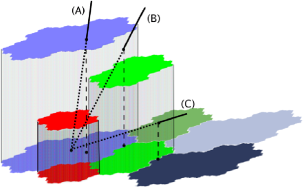
Figure 2. Illustration of the three cases of Theorem 4.11 and Proposition 4.15. We have chosen a unit Pisot number for the illustration of these three cases for the sake of clarity. By Proposition 4.15, $\gamma(\beta)$ is given by the largest part of the diagonal line to be fully included in the natural extension $\bigcup_{a\in{\mathcal{A}}}(-\widetilde{\mathcal{T}}^{(a)})\times[0,T_{\beta}^{(a-1)}(1))$. The natural extension is represented with subtiles $-\widetilde{\mathcal{T}}^{(a)}$ in the horizontal direction, and the interval $[0,1)$ in the vertical axis. Then, the natural extension consists in union of cylinders with fractal horizontal base and vertical height. The height of the cylinder with basis $-\widetilde{\mathcal{T}}^{(a)}$ is $T_{\beta}^{(a-1)}(1)$. Depending on the location of the point where the diagonal first goes out from the natural extension, we get the different situations unearthed in Theorem 4.11.
Situation (A) means that $\gamma(\beta)$ belongs to the orbit of $1$ under the action of $T_{\beta}$ and that its Euclidean embedding $\phi_{\infty}(\gamma(\beta))$ simultaneously is the Euclidean part of a point of the corresponding subtile. Then, the diagonal starts from 0 and exits from the natural extension on a plateau with height $T^{(a-1)}_{\beta}(1)$.
Situation (B) involves the intersection between two complete central subtiles tiles $(-\widetilde{\mathcal{T}}^{(a)})\cap(-\widetilde{\mathcal{T}}^{(b)})$. The diagonal line goes out from the natural extension on a vertical line above the intersection between two subtiles. The main point is that the plateau of the lowest cylinder ($T^{(b-1)}(1)$) lies below the diagonal line whereas the plateau of the upper cylinder ($T^{(a-1)}(1)$) lies above it.
Situation (C) means that the diagonal line completely crosses the natural extension and exits above a new $x$-tile.

Theorem 4.11 offhands yields lower and upper bounds for $\gamma(\beta)$.

Proposition 4.16.

We introduce some local notation. For $a$ and $b$ in ${\mathcal{A}}$ such that $T_{\beta}^{(b-1)}(1)\leq T_{\beta}^{(a-1)}(1)$, let

$$A_{a,b}=\pi_{\infty}\left(-\widetilde{\mathcal{T}}^{(a)}\cap-\widetilde{\mathcal{T}}^{(b)}\cap\left(\Delta_{\infty}([T_{\beta}^{(b-1)}(1),T_{\beta}^{(a-1)}(1)])\times\overline{\phi_{f}({\mathbb{Z}}_{(N(\beta))})}\right)\right)\subset{\mathbb{K}}_{\infty}.$$

For $a\in{\mathcal{A}}$ and $x\in{\mathbb{Z}}[1/\beta]$, let

$$B_{a,x}=\pi_{\infty}\left(-\widetilde{\mathcal{T}}^{(a)}\cap-\widetilde{\mathcal{T}}(x)\cap\left(\Delta_{\infty}((0,T_{\beta}^{(a-1)}(1)))\times\overline{\phi_{f}({\mathbb{Z}}_{(N(\beta))})}\right)\right)\subset{\mathbb{K}}_{\infty}.$$

Finally, let

$$A=\bigcup_{\genfrac{}{}{0.0pt}{1}{(a,b)\in{\mathcal{A}}^{2}}{T_{\beta}^{(b-1)}(1)\leq T_{\beta}^{(a-1)}(1)}}A_{a,b}\quad\textrm{and}\quad B=\bigcup_{\genfrac{}{}{0.0pt}{1}{a\in{\mathcal{A}}}{x\in{\mathbb{Z}}[1/\beta]\cap(0,1)}}B_{a,x}$$

Then, an upper bound for $\gamma(\beta)$ is given by

(4.7) $$\gamma(\beta)\geq\min\left(\min_{\begin{subarray}{c}(a,b)\in{\mathcal{A}}^{2}\\ T_{\beta}^{(b-1)}(1)\leq T_{\beta}^{(a-1)}(1)\\ A_{a,b}\neq\emptyset\end{subarray}}\min_{x\in A_{a,b}}\|\pi_{\infty}(x)\|_{\infty},\min_{\begin{subarray}{c}a\in{\mathcal{A}}\\ x\in{\mathbb{Z}}[1/\beta]\cap(0,1)\\ B_{a,x}\neq\emptyset\end{subarray}}\inf_{x\in B_{a,x}}\|\pi_{\infty}(x)\|_{\infty}\right).$$

A lower bound for $\gamma(\beta)$ is the following:

(4.8) $$\gamma(\beta)\leq\max\left\{\eta;\,[0,\eta]\subset A\cup B\right\}.$$

Proof.

First note that the infimum in (4.7) is due to the fact that $B_{a,x}$ does not need to be compact. We use Theorem 4.11 and the fact, that, by definition, $\gamma(\beta)$ is the largest number $\gimel$ such that $(0,\gimel)\cap{\mathbb{Z}}_{(N(\beta))}\subset\Pi_{\beta}^{(r)}$. Situation (A) in Theorem 4.11 implies that there exists $a\in{\mathcal{A}}$ such that $\gamma(\beta)=T_{\beta}^{(a-1)}(1)$ and $\gamma(\beta)\in\pi_{\infty}(-\widetilde{\mathcal{T}}^{(a)})$; it reads off that $\gamma(\beta)\in A_{a,a}$. Situation (B) implies that there exist $a,b\in{\mathcal{A}}$ with $T_{\beta}^{b-1}(1)<T_{\beta}^{a-1}(a)$ such that $\gamma(\beta)\in A_{a,b}$. However, the interval is closed in the present proposition, as it is half-closed in Theorem 4.11. Nevertheless, by continuity of $\pi_{\infty}$, taking open or closed intervals in $B_{a,x}$ or $A_{a,b}$ has no influence on the infimum we are interested in. Situation (C) reads off that there exist $a\in{\mathcal{A}}$ and $x\in{\mathbb{Z}}[1/\beta]\cap(0,1)$ such that $\gamma(\beta)\in B_{a,x}$. Since one the 3 situations must occur, we deduce that $\gamma(\beta)$ is greater than the smallest of the infimum of all these sets. Formulas (4.8) hold for the same reasons.

The three cases are illustrated in Fig. 2. ∎

4.5. Quadratic Pisot numbers

Let us now consider the particular case of quadratic Pisot numbers of degree 2, for which many things can be done explicitely. For instance, ${\mathbb{Q}}(\beta)$ is an extension of degree two, and then the algebraic conditions (3) or (4) of Proposition 4.9 can be easily tested. Indeed, let $d$ be the square-free positive rational integer such that ${\mathbb{Q}}(\beta)={\mathbb{Q}}(\sqrt{d})$. Then the discriminant $\delta_{{\mathbb{Q}}(\beta)}$ of the quadratic field is $d$ if $d\equiv 1\pmod{4}$ and $4d$ if $d\equiv 2,3\pmod{4}$.

Corollary 4.17.

If $\beta^{2}=a\beta+b$, with $(a,b)\in{\mathbb{Z}}^{2}$, $b\neq 0$, the equivalent conditions of Proposition 4.9 are satisfied if and only if:

1. $b$ is square free,

2. $b$ is coprime with $\delta_{{\mathbb{Q}}(\beta)}$,

3. $d$ is a quadratic residue with respect to all odd prime divisors of $b$,

4. $d\equiv 1\pmod{8}$ if $b$ is even.

The Euclidean representation space ${\mathbb{K}}_{\infty}$ is a one-dimensional line. Consequently, the diagonal $\Delta_{\infty}([0,\varepsilon])$ is indeed the interval $[0,\varepsilon]\subset{\mathbb{K}}_{\infty}={\mathbb{R}}$. This allows us to use graphical representation of the complete central tile to conjecture lower bounds for $\gamma(\beta)$.

A particularly manageable case is the following: $(\beta)=\beta\mathfrak{O}$ is a prime ideal lying above a prime number $p$, that splits. Hence $(\beta)$ has inertia degree 1, we have $N((\beta))=|N(\beta)|=p$, and ${\mathbb{K}}_{\beta}={\mathbb{R}}\times{\mathbb{Q}}_{p}$ (that is a special case of Corolary 4.17). We can represent ${\mathbb{Z}}_{p}$ by the Mona map ${\mathbb{Z}}_{p}\ni x=\sum a_{i}p^{i}\mapsto\sum a_{i}p^{-i}\in[0,1]$. This mapping is onto, continuous and preserves the Haar measure, but is it not a morphism for the addition. Corollary 4.8 implies that $\gamma(\beta)\geq\varepsilon$ if and only if a stripe of length $\varepsilon$ is totally included in the representation of the central tile, as illustrated by Fig. 3 and Fig. 4 below.

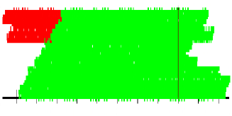
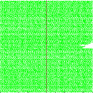
Figure 3. A representation of the complete central tile for $\beta=5+2\sqrt{7}$. Then $\beta$ has minimum polynomial $X^{2}-10X-3$ and $N((\beta))=-3$. The quadratic field ${\mathbb{Q}}(\beta)={\mathbb{Q}}(\sqrt{7})$ has discriminant 28, hence $\left(\frac{28}{3}\right)=\left(\frac{1}{3}\right)=1$: the discriminant is a quadratic residue modulo 3 and Corollary 4.17 shows that the complete central tile is a subset of ${\mathbb{R}}\times{\mathbb{Z}}_{3}$. The vertical axis stands for a representation of ${\mathbb{Z}}_{3}$ as embedded in $[0,1)$. The horizontal axis stands for the real line. Since $d_{\beta}(1)=1030^{\infty}$, there are two complete central subtiles (green and red). The right figure depicts a zoom along the vertical axis. This zoom seems to suggest that the central tile contains a full stripe of the form $[-\varepsilon,\varepsilon]\times{\mathbb{Z}}_{3}$, so that $\gamma(\beta)>0$.

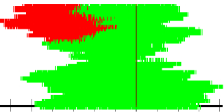
Figure 4. A representation of the complete central tile for the Pisot number satisfying $\beta^{2}=4\beta+3$. As in the previous case, we have ${\mathbb{Q}}(\beta)={\mathbb{Q}}(\sqrt{7})$ and $N((\beta))=-3$. Thus the complete central tile is again a subset of ${\mathbb{R}}\times{\mathbb{Z}}_{3}$. Since $d_{\beta}(1)=430^{\infty}$, there are two complete central subtiles (green and red). The zoom suggests that the complete central tile contains no stripe of the form $[-\varepsilon,\varepsilon]\times{\mathbb{Z}}_{3}$, so that $\gamma(\beta)=0$.

Let us recall ([FS92], Proposition 1 and Lemma 3) that the finitenes property (F) holds for any quadratic Pisot number $\beta$, and that those numbers are exactly the dominant root of the polynomials $X^{2}-aX-b$ with $a\geq b\geq 1$ or $q\geq 3$ and $-a+2\leq b\leq-1$. Consequently, we may apply Theorem 3.18, and the intersections between complete $x$-tiles determine their boundary, which have zero measure. The same property holds for the subtiles. We then use the fact that inner points of $x$-tiles and subtiles are exclusive to deduce an explicit formula for $\gamma(\beta)$.

Theorem 4.18.

If $\beta$ is quadratic, then $\gamma(\beta)$ is given by the formula (4.7), that is in that case an equality.

Proof.

First recall that since ${\mathbb{K}}_{\infty}$ is one-dimensional, one has $\Delta(x)=x$ for all $x\in[0,1]$. We use the notation introduced in Proposition 4.16. We have to show that the lower bound is an upper bound too. We will show the following:

If $$x\in{\mathbb{Z}}[1/\beta]\cap(0,1) -\widetilde{\mathcal{T}}(x)\cap(0,1)\times\overline{\phi_{f}({\mathbb{Z}}_{(N(\beta))})}\neq\emptyset$$ with , then

(4.9a) $$\gamma(\beta)\leq\inf\left\{\pi_{\infty}\left(-\widetilde{\mathcal{T}}(x)\cap(0,1)\times\overline{\phi_{f}({\mathbb{Z}}_{(N(\beta))})}\right)\right\}.$$

If $$a\in{\mathcal{A}} -\widetilde{\mathcal{T}}^{(a)}\cap[T_{\beta}^{(a-1)},1)\times\overline{\phi_{f}({\mathbb{Z}}_{(N(\beta))})}\neq\emptyset$$ with , then

(4.9b) $$\gamma(\beta)\leq\inf\left\{\pi_{\infty}\left(-\widetilde{\mathcal{T}}^{(a)}\cap(T_{\beta}^{(a-1)},1)\times\overline{\phi_{f}({\mathbb{Z}}_{(N(\beta))})}\right)\right\}.$$

Since $-\widetilde{\mathcal{T}}(x)\cap(0,1)\times\overline{\phi_{f}({\mathbb{Z}}_{(N(\beta))})}\supset B_{a,x}$ for every $a\in{\mathcal{A}}$ and $-\widetilde{\mathcal{T}}^{(a)}\cap[T_{\beta}^{(a-1)},1)\times\overline{\phi_{f}({\mathbb{Z}}_{(N(\beta))})}\supset A_{a,b}$ for every $b$ with $T_{\beta}^{(b-1)}(1)\leq T_{\beta}^{(a-1)}(1)$, the theorem will follow from (4.9). Notice that by continuity of $\pi_{\infty}$, taking open or closed intervals in $B_{a,x}$ or $A_{a,b}$ has no influence on the infimum we are interested in.

We begin with (4.9a). Let $x\in{\mathbb{Z}}[1/\beta]\cap(0,1)$. Let $z\in-\widetilde{\mathcal{T}}(x)\cap(0,1)\times\overline{\phi_{f}({\mathbb{Z}}_{(N(\beta))})}$. Since $\beta$ has degree 2, the property (F) is satisfied, and $\widetilde{\mathcal{T}}(x)$ is the closure of its subset of exclusive inner points by Proposition 3.17.

Let us fix $\varepsilon>0$. There exists an exclusive inner point $y\in-\widetilde{\mathcal{T}}(x)\setminus(-\widetilde{\mathcal{T}})$ such that $\|y-z\|\leq\varepsilon/2$. Since $y$ is an inner point and all inner points are exclusive, there exists $\nu<\varepsilon/2$ such that the ball $B(y,\nu)$ is contained in $-\widetilde{\mathcal{T}}(x)\setminus(-\widetilde{\mathcal{T}})$. By Lemma 4.7, the set $\phi_{\beta}((\pi_{\infty}(y)-\nu,\pi_{\infty}(y)+\nu)\cap{\mathbb{Z}}_{(N(\beta))})$ is dense in $[\pi_{\infty}(y)-\nu,\pi_{\infty}(y)+\nu]\times\overline{\phi_{f}({\mathbb{Z}}_{(N(\beta))})}$. Therefore, it intersects $B(y,\nu)$, and there exists $w\in(\pi_{\infty}(y)-\nu,\pi_{\infty}(y)+\nu)\cap{\mathbb{Z}}_{(N(\beta))}$ such that $\phi_{\beta}(w)\in-\widetilde{\mathcal{T}}(x)\setminus(-\widetilde{\mathcal{T}})$. For $w\leq\pi_{\infty}(z)+\varepsilon$, we know by Theorem 4.2 that the $\beta$-expansion of $w$ is not purely periodic. Hence $\gamma(\beta)\leq\pi_{\infty}(z)+\varepsilon$. Finally, $\gamma(\beta)\leq\pi_{\infty}(z)$ and (4.9a) is proved.

The proof for the upper bound (4.9b) follows the same lines. Let $z\in-\widetilde{\mathcal{T}}^{(a)}\cap(T_{\beta}^{(a-1)},1)\times\overline{\phi_{f}({\mathbb{Z}}_{(N(\beta))})}$. Then $\widetilde{\mathcal{T}}^{(a)}$ is the closure of its set of exclusive inner points (with respect to $\widetilde{\mathcal{T}}^{(b)}$, $b\neq a$). For $\varepsilon>0$, there exists an exclusive inner point $y$ and $\nu>0$ such that $B(y,\nu)\subset-\widetilde{\mathcal{T}}^{(a)}\setminus\bigcup_{b\in{\mathcal{A}}\setminus\{a\}}\widetilde{\mathcal{T}}^{(b)}$ and $(\pi_{\infty}(y)-\nu,\pi_{\infty}(y)+\nu)\subset(T_{\beta}^{(a-1)},1)$ (this second condition is the reason for which we take an open intervall in (4.9b)). By Lemma 4.7, there exists $w\in(\pi_{\infty}(y)-\nu,\pi_{\infty}(y)+\nu)\cap{\mathbb{Z}}_{(N(\beta))}$ such that $\phi_{\beta}(w)\in-\widetilde{\mathcal{T}}^{(a)}\setminus\bigcup_{b\in{\mathcal{A}}\setminus\{a\}}\widetilde{\mathcal{T}}^{(b)}$. Since $\pi_{\infty}(w)>T_{\beta}^{(a-1)}$, $w\not\in\Pi_{\beta}^{(r)}$. Therefore, $\gamma(\beta)\leq\pi_{\infty}(z)+\varepsilon$. Finally, $\gamma(\beta)\leq\pi_{\infty}(z)$ and (4.9b) is proved. ∎

Suppose that the degree of $\beta$ is larger than 2. We know that $\pi_{\infty}(\phi_{\beta}({\mathbb{Q}}\cap[0,1]))\subset\Delta_{\infty}([0,1])$. However, the diagonal set $\Delta_{\infty}([0,\infty))$ has empty interior in ${\mathbb{K}}_{\infty}$. Consequently, it may happen that $\pi_{\infty}(-\widetilde{\mathcal{T}}(x))$ is tangent to the diagonal $\Delta_{\infty}([0,\infty))$; in this latter case, $-\widetilde{\mathcal{T}}(x)$ provides no point with a non-periodic beta-expansion and the conclusion of Theorem 4.18 may fail.

5. Two quadratic examples

In the previous section, we have proved that $\gamma(\beta)$ is deeply related with the intersections between subtiles and $x$-tiles. In this section, we will detail on two examples how $\gamma(\beta)$ can be explicitely computed. To achieve this task, we will use the boundary graph defined in Section 3.4. In Corollary 3.13, we have proved that the boundary graph can be computed by three conditions (N1), (N3) and (N4). Conditions (N1) and (N4) are simple numerical conditions. On the contrary, condition (N3) implies the integer ring $\mathfrak{O}$. In order to check this condition, we need to find an explicit basis of ${\mathfrak{O}}\cap{\mathbb{Z}}[1/\beta]$. We thus introduce below a sufficient condition that reduces ${\mathfrak{O}}\cap{\mathbb{Z}}[1/\beta]$ to ${\mathbb{Z}}[\beta]$.

Lemma 5.1.

Let $\beta$ be such that $\beta{\mathfrak{O}}$ has only divisors of degree 1, and with inertia degree 1. Let $x\in{\mathbb{Z}}[1/\beta]$. If $\beta^{k}x\in{\mathfrak{O}}$, then $\beta^{k}x\in{\mathbb{Z}}[\beta]$.

Proof.

Let us expand $x$ as $x=a_{d-1}\beta^{d-1}+\dots+a_{0}+\dots+a_{-N}\beta^{-N}$, with $a_{i}\in{\mathbb{Z}}$ (it is not the $\beta$-expansion). If $N>k$, then $\beta^{N}x=\beta^{N-k}(\beta^{k}x)\in\beta^{N-k}{\mathfrak{O}}$. We deduce that $a_{-N}\in\beta^{N-k}{\mathfrak{O}}+\beta{\mathbb{Z}}[\beta]\subset\beta{\mathfrak{O}}$. Hence $a_{-N}\in\beta{\mathfrak{O}}\cap{\mathbb{Z}}$. Since $\beta{\mathfrak{O}}$ has only divisors of degree 1 and with inertia degree 1, $N(\beta)$ divides $a_{-N}$. From $N(\beta)/\beta\in{\mathbb{Z}}[\beta]$, we deduce that $a_{-N}/\beta\in{\mathbb{Z}}[\beta]$. Then $x$ admits an expansion of size at most $\beta^{-N+1}$: $x=b_{d-1}\beta^{d-1}+\cdots b_{0}+\cdots+b_{-N+1}\beta^{-N+1}$. We conclude by induction that $\beta^{k}x\in{\mathbb{Z}}[\beta]$. ∎

Let us stress the fact that if $\beta$ is a quadratic number that satisfies the conditions of Proposition  4.9, then Lemma 5.1 holds. In this case, Corollary 3.13 reads as follows to compute the boundary graph.

Corollary 5.2.

Suppose that $\beta$ is a quadratic number such that $\beta{\mathfrak{O}}$ has only divisors of degree 1 and inertia degree 1. Let $\beta^{2}=a\beta+b$ be its minimal polynomial. The boundary graph of $\beta$ can be explicitely computed as follows.

1. Consider all triplets $[a,x,b]$ such that $x=K+\beta L$, $(K,L)\in{\mathbb{Z}}^{2}$, with

   • $K\leq\frac{\beta-a+3a\beta-\beta^{2}-a^{2}}{(2\beta-a)(1+a-\beta)}$ and $L\leq\frac{1+2a-\beta}{(2\beta-a)(1+a-\beta)}$.

   • $-T_{\beta}^{(a-1)}(1)<x<T_{\beta}^{(b-1)}(1)$ and $a\not=b$ if $x=0$.

2. Put an edge betwenn two triplets $[a,x,b]$ and $[a_{1},x_{1},b_{1}]$ if there exists $q_{1}$ and $p_{1}$ such that

   • $x_{1}=\beta^{-1}(x+q_{1}-p_{1})$,

   • $a_{1}\xrightarrow{p_{1}}a$ and $b_{1}\xrightarrow{q_{1}}b$ are edges of the admissibility graph.

3. Recursively remove edges that have no outgoing edge.

Proof.

From the proof of Corollary 3.13, it is sufficient to exhibit a set that contains all the triplets $[a,x,b]$ satisfying conditions (N1), (N3) and (N4). Then the recursive deletion of edges will reduce the graph to the exact boundary graph. In this case, condition (N3) implies that $x\in{\mathbb{Z}}[\beta]$. Then we are looking for all $x$’s such that $x=K\beta+L$, with $K,L\in{\mathbb{Z}}$, and such that conditions (N1) and (N4) are satisfied. let $x_{2}$ denote the conjugate of $x$ and $\beta_{2}=a-\beta$ denote the conjugate of $\beta$. We obtain $K=(\beta_{2}x-\beta x_{2})/(\beta-\beta_{2})$ and $L=(x-x_{2})/(\beta-\beta_{2})$. Condition (N1) means that $x\leq 1$, and condition (N4) implies that $|x_{2}|\leq\frac{\lfloor\beta\rfloor}{1-|\beta_{2}|}=\frac{a}{1+a-\beta}$. We deduce that if $[a,x,b]$ satisfies the three conditions (N1), (N3) and (N4), then $x=K\beta+L$ with $K\leq\frac{\beta-a+3a\beta-\beta^{2}-a^{2}}{(2\beta-a)(1+a-\beta)}$ and $L\leq\frac{1+2a-\beta}{(2\beta-a)(1+a-\beta)}$. ∎

When $\beta^{2}=4\beta+3$ the bounds are $K\leq 11$ and $L\leq 3$. We deduce that the boundary graph contains 18 nodes (Fig. 5). If $[a,x,b]$ is a node of the boundary graph, we have $x\in\pm\{0,\beta-4,5-\beta,2\beta-10,2\beta-9\}$. When $\beta>1$ defined by $\beta^{2}=10\beta+3$, the bounds are $K\leq 14$ and $L\leq 2$. The boundary graph contains 8 nodes (see left side of Fig. 7). If $[a,x,b]$ is a node of the boundary graph, we have $x\in\pm\{0,11-\beta,\beta-10\}$.

Proposition 5.3.

Let $\beta>1$ defined by $\beta^{2}=4\beta+3$. There are 9 non-empty intersections between the central subtiles and the neighbouring $x$-tiles, namely $\widetilde{\mathcal{T}}^{(1)}\cap\widetilde{\mathcal{T}}^{(2)}$, $\widetilde{\mathcal{T}}^{(1)}\cap(\widetilde{\mathcal{T}}^{(1)}+\phi_{\beta}(2\beta-9))$, $\widetilde{\mathcal{T}}^{(1)}\cap(\widetilde{\mathcal{T}}^{(2)}+\phi_{\beta}(2\beta-9))$, $\widetilde{\mathcal{T}}^{(1)}\cap(\widetilde{\mathcal{T}}^{(1)}+\phi_{\beta}(\beta-4))$, $\widetilde{\mathcal{T}}^{(2)}\cap(\widetilde{\mathcal{T}}^{(1)}+\phi_{\beta}(\beta-4))$, $\widetilde{\mathcal{T}}^{(1)}\cap(\widetilde{\mathcal{T}}^{(1)}+\phi_{\beta}(5-\beta))$, $\widetilde{\mathcal{T}}^{(2)}\cap(\widetilde{\mathcal{T}}^{(1)}+\phi_{\beta}(5-\beta))$, $\widetilde{\mathcal{T}}^{(1)}\cap(\widetilde{\mathcal{T}}^{(2)}+\phi_{\beta}(5-\beta))$ $\widetilde{\mathcal{T}}^{(2)}\cap(\widetilde{\mathcal{T}}^{(1)}+\phi_{\beta}(10-2\beta))$. The expansions of the points lying in one of those intersections are constrained by the graph depicted in Fig. 6.

Proof.

In order to obtain the interesting intersections, we consider in the boundary graph the subgraph of paths starting from $[a,x,b]$ with $x\in[0,T_{\beta}^{(b-1)}(1)[$ and $a<b$ if $x=0$. In the boundary graph, there are 9 nodes which satisfy these conditions: $[1,0,2]$, $[1,2\beta-9,1]$, $[1,2\beta-9,2]$, $[1,\beta-4,1]$, $[2,\beta-4,1]$, $[1,-\beta+5,1]$, $[1,-\beta+5,2]$, $[2,-\beta+5,1]$, $[2,-2\beta+10,1]$. From these nodes, infinite paths span a subgraph with 15 nodes, depicted in Fig. 6. ∎

Figure 5. The boundary graph for $\beta^{2}=4\beta+3$.

Figure 6. Subgraph of the boundary graph for $\beta^{2}=4\beta+3$ that gather infinite paths starting from a node $[a,x,b]$ with $x\in{\mathbb{Z}}[1/\beta]$, $0\leq x<T^{(b-1)}(1)$ and $a<b$ if $x=0$. These nodes are $[1,0,2]$, $[1,2\beta-9,1]$, $[1,2\beta-9,2]$, $[1,\beta-4,1]$, $[2,\beta-4,1]$, $[1,-\beta+5,1]$, $[1,-\beta+5,2]$, $[2,-\beta+5,1]$, $[2,-2\beta+10,1]$. They exacly stand for the set of intersections that contribute to the computation of $\gamma(\beta)$ in Proposition 4.16.

We obtain another graph for $\beta^{2}=10\beta+3$.

Proposition 5.4.

Let $\beta>1$ defined by $\beta^{2}=10\beta+3$. There are exactly 4 non-empty intersection between the central subtiles and $x$-tiles, namely $\widetilde{\mathcal{T}}^{(1)}\cap\widetilde{\mathcal{T}}^{(2)}$, $\widetilde{\mathcal{T}}^{(1)}\cap(\widetilde{\mathcal{T}}^{(1)}+\phi_{\beta}(\beta-10))$, $\widetilde{\mathcal{T}}^{(1)}\cap(\widetilde{\mathcal{T}}^{(1)}+\phi_{\beta}(-\beta+11))$, $\widetilde{\mathcal{T}}^{(2)}\cap(\widetilde{\mathcal{T}}^{(1)}+\phi_{\beta}(-\beta+11))$. The expansions of the points lying in one of those intersections are constrained by the graph depicted in Fig. 7.

Proof.

In the boundary graph, nodes $[a,x,b]$ that satisfy the condition $x\in[0,T_{\beta}^{(b-1)}(1)[$ and $a<b$ if $x=0$ are $[1,0,2]$, $[1,\beta-10,1]$, $[1,11-\beta,1]$ and $[2,11-\beta,1]$. In the boundary graph, paths starting from these nodes cover a subgraph with 5 nodes, shown in Fig. 7. ∎

Figure 7. (Left) The boundary graph for $\beta^{2}=10\beta+3$. The notation $B$ stands for $\beta$.
(Right) Subgraph of the boundary graph that gathers infinite paths starting from a node $[a,x,b]$ with $x\in{\mathbb{Z}}[1/\beta]$, $0\leq x<T^{(b-1)}(1)$ and $a<b$ if $x=0$. These nodes are $[1,0,2]$, $[1,\beta-10,1]$, $[1,11-\beta,1]$ and $[2,11-\beta,1]$. They exacly stand for the set of intersections that contribute to the computation of $\gamma(\beta)$ in Proposition 4.16.

We now have the tools to compute $\gamma(\beta)$ in some specific cases.

Lemma 5.5.

Let $\beta^{2}=4\beta+3$. We recall that $\pi_{\infty}$ stands for the projection from ${\mathbb{K}}_{\infty}$ to ${\mathbb{R}}$. Then

$$\pi_{\infty}\left(\widetilde{\mathcal{T}}^{(1)}\cap(\widetilde{\mathcal{T}}^{(1)}+\phi_{\beta}(\beta-4))\right)=\left\{\sum a_{i}{\beta_{2}}^{i}\ |\ a_{2i}\in\{0,1,2\},a_{2i+1}\in\{2,3,4\}\right\}.$$

Proof.

We use the boundary subgraph depicted in Fig. 6. By construction, any point of the intersection ${\widetilde{\mathcal{T}}}^{(1)}\cap\left(\widetilde{\mathcal{T}}^{(1)}+\phi_{\beta}(\beta-4)\right)$ can be expanded as $z=\sum_{i\geq 0}p_{i}\phi_{\beta}(\beta^{i})$, where $(p_{i})$ is the first coordinate of the labeling of a path starting in $[1,\beta-4,1]$. By looking at paths starting from $[1,\beta-4,1]$ we check in the graph that such sequences $(p_{i})$’s satisfy $p_{2i}\in\{0,1,2\}$ and $p_{2i+1}\in\{2,3,4\}$. Conversely, we also check that every sequence of this form is the first coordinate of the labeling of a path starting in $[1,\beta-4,1]$ in the graph. This yields

$$\pi_{\infty}(\widetilde{\mathcal{T}}^{(1)}\cap(\widetilde{\mathcal{T}}^{(1)}+\phi_{\beta}(\beta-4)))=\left\{\sum_{i\geq 0}\{0,1,2\}\beta_{2}^{2i}+\sum_{i\geq 0}\{2,3,4\}\beta_{2}^{2i+1}\right\}.$$

∎

In order to compute $\gamma(\beta)$, we use the following folklore lemma.

Lemma 5.6 (Cookie Cantor Lemma).

Let $\alpha<1$ be an integer number

$$X(\alpha,n):=\left\{\left.\sum_{i\geq 0}a_{i}\alpha^{i}\right|a_{i}\in\{0,1,\dots,n-1\}\right\}\subset\left[0,\frac{n-1}{1-\alpha}\right]$$

The two end points $\{0,\frac{n-1}{1-\alpha}\}$ belong to $X(\alpha,n)$. Furthermore, if $\alpha>1/n$, then it is a Cantor cookie cutter set and if $\alpha\in[1/n,1)$, then $X(\alpha,n)$ coincides with the interval $\left[0,(n-1)/(1-\alpha)\right]$.

Proof.

The set $X(\alpha,n)$ is the attractor of the IFS: $X=\bigcup_{i=0}^{n-1}\alpha X+i$ which has a unique non-empty compact solution. It is easy to see that the right hand side is a solution if $\alpha\in[1/n,1)$. ∎

Theorem 5.7.

One has

$$\gamma(2+\sqrt{7})=0.$$

Proof.

If $\beta^{2}=4\beta+3$ and $\beta$ is a Pisot number, then $\beta=2+\sqrt{7}$. We also check that $\beta$ satisfies the conditions of Corollary 4.17, hence $\overline{\phi_{f}({\mathbb{Z}}_{(N(\beta))})}={\mathbb{Z}}_{3}$. In this case, the set $A_{a,b}$ and $B_{a,x}$ in Proposition 4.16 simply correspond to intersections between tiles, with no more diagonal set: $A_{a,b}=\pi_{\infty}(-\widetilde{\mathcal{T}}^{(a)}\cap-\widetilde{\mathcal{T}}^{(b)}\cap[T_{\beta}^{(b-1)}(1),T_{\beta}^{(a-1)}(1)])\times{\mathbb{Z}}_{3})$ and $B_{a,x}=\pi_{\infty}(-\widetilde{\mathcal{T}}^{(a)}\cap-\widetilde{\mathcal{T}}(x)\cap(0,T_{\beta}^{(a-1)}(1))\times{\mathbb{Z}}_{3})$. Then computing $\gamma(\beta)$ reduced to understanding intersections between tiles.

Let $-\alpha$ denote the conjugate of $\beta$, that is, $\alpha=\sqrt{7}-2>1/3$. Lemma 5.5 exhibits a set that we need to compute explicitly.

$$\pi_{\infty}\left(\widetilde{\mathcal{T}}^{(1)}\cap(\widetilde{\mathcal{T}}^{(1)}+\phi_{\beta}(\beta-4))\right) = \left\{\sum a_{i}{\alpha}^{2i}-\sum b_{i}{\alpha}^{2i+1}\ |\ a_{i}\in\{0,1,2\},b_{i}\in\{2,3,4\}\right\}$$

$$= \left\{\sum a_{i}\alpha^{2i}+\sum c_{i}\alpha^{2i+1}\ |\ a_{i}\in\{0,1,2\},c_{i}\in\{-2,-3,-4\}\right\}$$

$$= X(\alpha,3)-\alpha(4+4\alpha^{2}+4\alpha^{4}+\dots)$$

$$= \left[-\frac{4\alpha}{1-\alpha^{2}},-\frac{4\alpha}{1-\alpha^{2}}+\frac{2}{1-\alpha}\right]$$

$$= \left[-\frac{4\alpha}{1-\alpha^{2}},\frac{2-2\alpha}{1-\alpha^{2}}\right]\ni 0$$

Hence zero is the minimum of $[0,T_{\beta}(1)]\cap\pi_{\infty}(-\widetilde{\mathcal{T}}^{(1)}\cap(-\widetilde{\mathcal{T}}(\beta-4))$ and Theorem 4.18 implies that $\gamma(\beta)=0$. ∎

A completely different behaviour appears when modifying only one digit in the quadratic equation satisfied by $\beta$.

Theorem 5.8.

One has

$$\gamma(5+2\sqrt{7})=\frac{7-\sqrt{7}}{12}$$

Proof.

The number $5+2\sqrt{7}$ is the root of $\beta^{2}-10\beta-3=0$. As before, conditions of Corollary 4.17 are satisfied hence $\overline{\phi_{f}({\mathbb{Z}}_{(N(\beta))})}={\mathbb{Z}}_{3}$, and studying intersections between tiles is enough to compute $\gamma(\beta)$.

From the graph depicted in Fig. 7, we deduce that non-empty intersections in the numeration tiling are given by $\widetilde{\mathcal{T}}^{(1)}\cap(\widetilde{\mathcal{T}}^{(2)}$, $\widetilde{\mathcal{T}}^{(1)}\cap(\widetilde{\mathcal{T}}^{(1)}+\phi_{\beta}(11-\beta))$, $\widetilde{\mathcal{T}}^{(2)}\cap(\widetilde{\mathcal{T}}^{(1)}+\phi_{\beta}(11-\beta))$, and $\widetilde{\mathcal{T}}^{(1)}\cap(\widetilde{\mathcal{T}}^{(1)}+\phi_{\beta}(+10+\beta))$.

We can detail the expansion of the real projection of the three last sets.

$$\pi_{\infty}(\widetilde{\mathcal{T}}^{(1)}\cap(\widetilde{\mathcal{T}}^{(1)}+\phi_{\beta}(11-\beta)))=\{8,9\}+\beta_{2}\sum_{i\geq 0}\{0,1,2\}\beta_{2}^{2i}+\{8,9,10\}\beta_{2}^{2i+1}$$

$$\pi_{\infty}(\widetilde{\mathcal{T}}^{(2)}\cap(\widetilde{\mathcal{T}}^{(1)}+\phi_{\beta}(11-\beta)))=10+\beta_{2}\sum_{i\geq 0}\{0;1,2\}\beta_{2}^{2i}+\{8,9,10\}\beta_{2}^{2i+1}$$

$$\pi_{\infty}(\widetilde{\mathcal{T}}^{(1)}\cap(\widetilde{\mathcal{T}}^{(1)}+\phi_{\beta}(-10+\beta)))=\{0,1,2\}+\beta_{2}\sum_{i\geq 0}\{8,9,10\}\beta_{2}^{2i}+\{0,1,2\}\beta_{2}^{2i+1}$$

We use the Cookie Cantor Lemma stated above with $\alpha=-\beta_{(2)}=3\beta^{-1}$ and $n=3>\alpha^{-1}$ to compute the sum that is involved in each intersection.

$$\sum_{i\geq 1}\{0,1,2\}\beta_{2}^{2i}+\{8,9,10\}\beta_{2}^{2i+1} = \sum_{i\geq 0}\{0;1,2\}\alpha^{2i}-\{8,9,10\}\alpha^{2i+1}$$

$$= -10\sum_{i\geq 0}\alpha^{2i+1}+\sum_{j\geq 0}\{0,1,2\}\alpha^{j}$$

$$= \frac{-10\alpha}{1-\alpha^{2}}+\left[0,\frac{2}{1-\alpha}\right]=\left[\frac{-10\alpha}{1-\alpha^{2}},\frac{-8\alpha+2}{1-\alpha^{2}}\right]$$

Similarly, we have

$$\sum_{i\geq 1}\{8,9,10\}\beta_{2}^{2i}+\{0,1,2\}\beta_{2}^{2i+1} = 10\sum_{i\geq 0}\alpha^{2i}-\sum_{j\geq 0}\{0,1,2\}\alpha^{j}$$

$$= \frac{10}{1-\alpha^{2}}-\left[0,\frac{2}{1-\alpha}\right]=\left[\frac{8-2\alpha}{1-\alpha^{2}},\frac{10}{1-\alpha^{2}}\right].$$

We deduce that

$$\pi_{\infty}(\widetilde{\mathcal{T}}^{(1)}\cap(\widetilde{\mathcal{T}}^{(1)}+\phi_{\beta}(11-\beta)))=\left[8-\alpha\frac{-8\alpha+2}{1-\alpha^{2}},8-\alpha\frac{-10\alpha}{1-\alpha^{2}}\right]\subset\left]0,\infty\right[.$$

Hence $-\pi_{\infty}(\widetilde{\mathcal{T}}\cap(\widetilde{\mathcal{T}}^{(1)}+\phi_{\beta}(11-\beta)))\cap[0,1]=\emptyset$. Similarly, we have $-\pi_{\infty}(\widetilde{\mathcal{T}}\cap(\widetilde{{\mathcal{T}}^{(2)}}+\phi_{\beta}(11-\beta)))\cap[0,1]=\emptyset$, so that both intersections cannot be taken into account in the computation of $\gamma(\beta)$. This implies that $-\pi_{\infty}(\widetilde{\mathcal{T}}^{(2)})\cap[0,\infty]$ does not intersect the projection of any tile $-\pi_{\infty}(\widetilde{\mathcal{T}}(x))$.

We also have

$$\pi_{\infty}(\widetilde{\mathcal{T}}^{(1)}\cap(\widetilde{\mathcal{T}}^{(1)}+\phi_{\beta}(\beta-10)))=\left[\frac{-10\alpha}{1-\alpha^{2}},\frac{-8\alpha+2}{1-\alpha^{2}}\right].$$

Hence, the minimum of $-\pi_{\infty}(\widetilde{\mathcal{T}}^{(1)}\cap(\widetilde{\mathcal{T}}^{(1)}+\phi_{\beta}(\beta-10)))$ is $\frac{8\alpha-2}{1-\alpha^{2}}$.

In order to apply Theorem 4.18, we prove that the infimum of intersections of the form $\pi_{\infty}(A_{a,b})$ (situation (A) or (B)) is strictly larger than the infimum of intersections $\pi_{\infty}(B_{x,a})$ (situation (C)). By definition, we have $\pi_{\infty}(\widetilde{\mathcal{T}}^{(2)})=\{\sum_{i\geq 0}a_{2i}\alpha^{2}i-\sum_{i\geq 0}a_{2i+1}\alpha^{2i+1}\}$ where sequences $a_{1}\dots a_{i}\dots$ are sequences starting from 2 in the reverse of the admissibility graph. We deduce that $a_{0}=10$, $a_{1}\leq 9$, $a_{2}\geq 0$, and then, $a_{2i+2}\geq 0$ and $a_{2i+3}\leq 10$. Hence

$$\min\pi_{\infty}(\widetilde{\mathcal{T}}^{(2)})\geq 10-9\alpha+0\alpha^{2}-10\alpha^{3}+\dots=10-9\alpha+10\frac{\alpha^{3}}{1-\alpha^{2}}>0.$$

Consequently, $-\pi_{\infty}(\widetilde{\mathcal{T}}^{(2)})\cap[0,\infty]=\emptyset$ and situations (A) or (B) do not contribute to $\gamma(\beta)$.

From Theorem 4.18, we deduce that $\gamma(\beta)=\min-\pi_{\infty}(\widetilde{\mathcal{T}}^{(1)}\cap(\widetilde{\mathcal{T}}^{(1)}+\phi_{\beta}(11-\beta)))=\frac{8\alpha-2}{1-\alpha^{2}}=\frac{7-\sqrt{7}}{12}$. ∎

6. Perspectives

At least two main directions deserve now to be discussed. In the quadratic case, what is the structure of the intersection graph allowing to compute $\gamma(\beta)$? The first question is whether we can obtain an algorithmic way to compute $\gamma(\beta)$ for every quadratic $\beta$. Then, can we deduce a general formula for $\gamma(\beta)$ for subfamilies of $\beta$? The first step would be to describe properly the structure of the boundary graph, at least for the family $\beta^{2}=n\beta+3$.

Another direction lies in the application of these methods in the three (or more dimensional case), including the unit case. At the moment we cannot give an explicit formula for $\gamma(\beta)$. In order to generalise the results to higher degrees, an approximation of exclusive inner points by the diagonal line of ${\mathbb{K}}_{\beta}$ is needed. This seems reasonable at least in the unit case, but requires a precise study of the topology of the central tile. Examples of computations of intersections between line and fractals are obtained in [AS05], by numeric approximations. As an example, an intersection is prove to be approximated by 0.66666666608644067488. Then it is not equal to 2/3, though very near from it. Theorem 5.8 is an example where we were able to compute explicitely the value of $\gamma(\beta)$ and it turned out that $\gamma(\beta)\in{\mathbb{Q}}(\beta)$. The question of the algebraic nature of $\gamma(\beta)$ in general is interesting.

References

- [Aki98] S. Akiyama. Pisot numbers and greedy algorithm. In Number theory (Eger, 1996), pages 9–21. de Gruyter, Berlin, 1998.
- [Aki00] S. Akiyama. Cubic Pisot units with finite beta expansions. In Algebraic number theory and Diophantine analysis (Graz, 1998), pages 11–26. de Gruyter, Berlin, 2000.
- [Aki02] S. Akiyama. On the boundary of self affine tilings generated by Pisot numbers. J. Math. Soc. Japan, 54(2):283–308, 2002.
- [Aki07] S. Akiyama. Pisot number system and its dual tiling. In Physics and Theoretical Computer Science (Cargese, 2006), pages 133–154. IOS Press, 2007.
- [AS05] S. Akiyama and K. Scheicher. Intersecting two dimensional fractals and lines. Acta Sci. Math. (Szeged), 3-4:555–580, 2005.
- [BBLT06] G. Barat, V. Berthé, P. Liardet, and J. M. Thuswaldner. Dynamical directions in numeration. Ann. Inst. Fourier (Grenoble), 56(7):1987–2092, 2006.
- [Ber77] A. Bertrand. Développements en base de Pisot et répartition modulo . C. R. Acad. Sci. Paris Sér. A-B, 285(6):A419–A421, 1977.
- [BFGK98] Č. Burdík, Ch. Frougny, J. P. Gazeau, and R. Krejcar. Beta-integers as natural counting systems for quasicrystals. J. Phys. A, 31(30):6449–6472, 1998.
- [Bla89] F. Blanchard. -expansions and symbolic dynamics. Theoret. Comput. Sci., 65(2):131–141, 1989.
- [BS05] V. Berthé and A. Siegel. Tilings associated with beta-numeration and substitutions. Integers, 5(3):A2, 46 pp. (electronic), 2005.
- [BS07] V. Berthé and A. Siegel. Purely periodic -expansions in the Pisot non-unit case. To appear, 2007.
- [CF86] J. W. S. Cassels and A. Fröhlich, editors. Algebraic number theory, London, 1986. Academic Press Inc.
- [CFS82] I. P. Cornfeld, S. V. Fomin, and Ya. G. Sinaĭ. Ergodic theory, volume 245 of Grundlehren der Mathematischen Wissenschaften [Fundamental Principles of Mathematical Sciences]. Springer-Verlag, New York, 1982. Translated from the Russian by A. B. Sosinskiĭ.
- [DKS96] K. Dajani, C. Kraaikamp, and B. Solomyak. The natural extension of the -transformation. Acta Math. Hungar., 73(1-2):97–109, 1996.
- [Fro00] C. Frougny. Number representation and finite automata. In Topics in symbolic dynamics and applications (Temuco, 1997), volume 279 of London Math. Soc. Lecture Note Ser., pages 207–228. Cambridge Univ. Press, 2000.
- [FS92] C. Frougny and B. Solomyak. Finite beta-expansions. Ergodic Theory Dynamical Systems, 12:45–82, 1992.
- [HI97] M. Hama and T. Imahashi. Periodic -expansions for certain classes of Pisot numbers. Comment. Math. Univ. St. Paul., 46(2):103–116, 1997.
- [IR04] S. Ito and H. Rao. Purely periodic -expansions with Pisot unit base. Proc. Amer. Math. Soc., 133(4):953–964 (electronic), 2004.
- [Lot02] M. Lothaire. Algebraic combinatorics on words, volume 90 of Encyclopedia of Mathematics and its Applications. Cambridge University Press, Cambridge, 2002. (Chapter 7, written by C. Frougny).
- [Par60] W. Parry. On the -expansions of real numbers. Acta Math. Acad. Sci. Hungar., 11:401–416, 1960.
- [Pra99] B. Praggastis. Numeration systems and Markov partitions from self-similar tilings. Trans. Amer. Math. Soc., 351(8):3315–3349, 1999.
- [QRY05] Y.-H Qu, H. Rao, and Y.-M. Yang. Periods of -expansions and linear recurrent sequences. Acta Arith., 120(1):27–37, 2005.
- [Rau88] G. Rauzy. Rotations sur les groupes, nombres algébriques, et substitutions. In Séminaire de Théorie des Nombres, 1987–1988 (Talence, 1987–1988). Univ. Bordeaux I, Talence., 1988. Exp. No. 21, 12.
- [Roh61] V. A. Rohlin. Exact endomorphisms of a Lebesgue space. Izv. Akad. Nauk SSSR Ser. Mat., 25:499–530, 1961.
- [San02] Y. Sano. On purely periodic beta-expansions of Pisot numbers. Nagoya Math. J., 166:183–207, 2002.
- [Sch80] K. Schmidt. On periodic expansions of Pisot numbers and Salem numbers. Bull. London Math. Soc., 12(4):269–278, 1980.
- [Sie03] A. Siegel. Représentation des systèmes dynamiques substitutifs non unimodulaires. Ergodic Theory Dynam. Systems, 23(4):1247–1273, 2003.
- [Sin06] Bernd Sing. Iterated function systems in mixed Euclidean and -adic spaces. In Complexus mundi, pages 267–276. World Sci. Publ., Hackensack, NJ, 2006.
- [ST07] A. Siegel and J. M. Thuswaldner. Topological properties of rauzy fractals. preprint, 2007.
- [SW02] V. F. Sirvent and Y. Wang. Self-affine tiling via substitution dynamical systems and Rauzy fractals. Pacific J. Math., 206(2):465–485, 2002.
- [Thu89] W. P. Thurston. Groups, tilings and finite state automata. In AMS Colloquium lectures. AMS Colloquium lectures, 1989.
- [Thu06] Jörg M. Thuswaldner. Unimodular Pisot substitutions and their associated tiles. J. Théor. Nombres Bordeaux, 18(2):487–536, 2006.