Computer Based Analytical Simulations of the Chiral Hadronic Processes

Abstract

The availability of computational modeling tools for subatomic physics (Form, FeynArts, FormCalc, and FeynCalc) has made it possible to perform sophisticated calculations in perturbative quantum field theory. We have adapted these packages in order to apply them to the effective chiral field theory of hadronic interactions. A detailed description of this Computational Hadronic Model is presented here, along with sample calculations.

I Introduction

Chiral Perturbation Theory (ChPT) has been tremendously successful in describing low-energy hadronic interactions in the non-perturbative regime of QCD. It provides for a systematic and well-defined perturbative expansion incorporating interaction physics driven by the symmetries of QCD in kinematic regimes where scales are well-defined.

Calculations have been performed for many problems to Next-to-Leading-Order (NLO) in a variety of bases, but the challenge is often in determining the range of valid and contributing degrees of freedom to a given problem.

With recent developments in the automatization of the NLO calculations in perturbative field theory, it is reasonable to consider the possibility that these methods could also be applied to ChPT and thus allow for a broader application of the theory.

To date, there are several packages available (FeynArts (FeynArts, ), FormCalc (FormCalc, ), FeynCalc (FeynCalc, ) and Form (Form, )) allowing us to produce semi-automatic calculations in particle physics. These packages have been applied in various calculations relevant to studies of the Standard Model (BeD94, ; DeDH97, ; DeH98, ; GuHK99, ; HoS99, ; Ha00, ).

Although FeynArts and FormCalc were originally designed for Standard Model calculations, the flexibility of the programs allows us to extend them to interactions appropriate for the hadronic sector. This was a main reason to use FeynArts and FormCalc as a base languages for the automatization of chiral hadronic calculations. Hence the main purpose of this work is to develop an extension to FeynArts and FormCalc which will perform automatic analytical calculations in ChPT.

We will begin by presenting a summary of the properties of Chiral Perturbation Theory, followed by a description of how the interactions can be incorporated into a computational hadronic model. We will then present some sample applications and tests of the model, along with plans for future development.

II Effective Chiral Lagrangian

Let us start with a general review of the formalism we use to describe the dynamics of the strong interactions. Spontaneous symmetry breaking of $SU\left(3\right)_{L}\otimes SU\left(3\right)_{R}$ due to the pseudo-Goldstone scalar bosons into $SU\left(3\right)_{V}$ can be described by the Lagrangian from

$$\mathfrak{L_{\pi\pi}^{(8)}}=\frac{f_{\pi}^{2}}{8}Tr\left[D^{\mu}{\textstyle\sum\nolimits^{\dagger}}D_{\mu}{\textstyle\sum}\right].$$ (1)

Eq.(1) represents the first term of the effective Lagrangian from (Manohar1991, ), which is the only allowed term with two derivatives. And additional term $Tr{\textstyle\sum\nolimits^{\dagger}}{\textstyle\sum}$ is a constant due to the equivalence theorem and is excluded from the effective Lagrangian. Here, $f_{\pi}\approx 135\,MeV$ is the pion decay constant and ${\textstyle\sum}$ field is given by

$${\textstyle\sum}=e^{2iP/f_{\pi}},$$ (2)

where $P$ is the pseudo-Goldstone boson octet:

$$P=\left(\begin{array}[]{ccc}\frac{1}{\sqrt{6}}\eta+\frac{1}{\sqrt{2}}\pi&\pi^{+}&K^{+}\\ \pi^{-}&\frac{1}{\sqrt{6}}\eta-\frac{1}{\sqrt{2}}\pi&K^{0}\\ K^{-}&\bar{K}^{0}&-\frac{2}{\sqrt{6}}\eta\end{array}\right).$$ (3)

Taking into account $U\left(1\right)_{Q}$ of electromagnetism, the covariant derivative is given by

$$D_{\mu}=\partial_{\mu}+i\mathcal{A}_{\mu}\left[Q,...\right],$$ (4)

where $\mathcal{A}$ enters as the electromagnetic vector field potential and $Q$ is a charge operator. Unlike the baryon field, chiral symmetry transformation for the pseudo-Goldstone boson field exists and is well defined as ${\textstyle\sum}\rightarrow L{\textstyle\sum}R^{\dagger}$. To introduce baryon field into the effective Lagrangian uniquely, the new field $\xi$ is defined as $\xi^{2}={\textstyle\sum}$. The chiral symmetry transformations for the field $\xi$ can be determined in the a new basis $U$ (see (Manohar1993, )) as

$$\xi\rightarrow L\xi U^{\dagger}=U\xi R^{\dagger}.$$ (5)

Here, the unitary matrix $U$ is implicitly defined from Eq.(5) in terms of $L,\,R,\,$and $\xi$, and in this case the chiral transformation for the baryon field is unique, and chosen to be $B\rightarrow UBU^{\dagger}.$ Choice of the basis $U$ is preferable for the effective Lagrangian with baryons, because in this basis pions are coupled through the derivative type coupling only. Consequently, the effective Lagrangian for the baryons can be written in terms of the vector fields (vector $V_{\mu}$ and axial-vector $A_{\mu}$):

$$V_{\mu} =\frac{1}{2}\left(\xi D_{\mu}\xi^{\dagger}+\xi^{\dagger}D_{\mu}\xi\right)=\frac{1}{f_{\pi}^{2}}\left[P,\partial_{\mu}P\right]+\frac{1}{f_{\pi}^{4}}\left[P,P\left(\partial_{\mu}P\right)P\right]+...,$$

$$A_{\mu} =\frac{i}{2}\left(\xi D_{\mu}\xi^{\dagger}-\xi^{\dagger}D_{\mu}\xi\right)=\frac{1}{f_{\pi}}\partial_{\mu}P+\frac{1}{f_{\pi}^{3}}P\left(\partial_{\mu}P\right)P-\frac{1}{2f_{\pi}^{3}}\left\{\partial_{\mu}P,P^{2}\right\}.$$

The leading order baryon Lagrangian is given by (Manohar1993, )

$$\mathfrak{L}_{B\pi}^{(8)}=-iTr\,\bar{B}\mathfrak{\not D}B+m_{B}Tr\,\bar{B}B+2D\,Tr\,\bar{B}\gamma^{\mu}\gamma_{5}\left\{A_{\mu},B\right\}+2F\,Tr\,\bar{B}\gamma^{\mu}\gamma_{5}\left[A_{\mu},B\right],$$ (7)

where $B$ is $SU\left(3\right)$ octet of baryons given by

$$B=\left(\begin{array}[]{ccc}\frac{1}{\sqrt{2}}\sum^{0}+\frac{1}{\sqrt{6}}\Lambda&\sum^{+}&p\\ \sum^{-}&-\frac{1}{\sqrt{2}}\sum^{0}+\frac{1}{\sqrt{6}}\Lambda&n\\ \Xi^{-}&\Xi^{0}&-\frac{2}{\sqrt{6}}\Lambda\end{array}\right),$$ (8)

with covariant derivative defined as $\mathfrak{\not D=}\partial_{\mu}+[V_{\mu},...].$ The strong coupling constants $\left\{F,D\right\}$ of the Lagrangian from Eq.(7) have been determined in (Manohar1991, ) to be $F=0.40\pm 0.03$ and $D=0.61\pm 0.04$. At the lowest order of chiral perturbation theory, the strong interaction of the decuplet $T_{\mu}$$\left(J^{P}=3/2^{\pm}\right)$ can be described by the following Lagrangian:

$$\mathfrak{L}_{T\pi}^{(10)}=-i\bar{T}^{\mu}\mathfrak{\not D}T_{\mu}+m_{T}\bar{T}^{\mu}T_{\mu}+\mathcal{C}\left(\bar{B}A_{\mu}\Gamma_{5}T^{\mu}+\bar{T}^{\mu}A_{\mu}\Gamma_{5}B\right)+2\mathcal{H}\bar{T}^{\mu}\gamma^{\nu}\gamma_{5}A_{\nu}\Gamma_{5}T_{\mu},$$ (9)

where $\Gamma_{5}=1$ for $T_{\mu}^{J^{P}=3/2^{+}}$ and $\Gamma_{5}=\gamma_{5}$ for $T_{\mu}^{J^{P}=3/2^{-}}$. The decuplet states $T_{\mu}$ are given by

$$T^{333} =\Omega^{-},$$

$$T^{133} =\frac{1}{\sqrt{3}}\Xi^{\ast 0},\,T^{233}=\frac{1}{\sqrt{3}}\Xi^{\ast-},$$

$$T^{113} =\frac{1}{\sqrt{3}}\sum\nolimits^{\ast+},\,T^{123}=\frac{1}{\sqrt{6}}\sum\nolimits^{\ast 0},\,T^{223}=\frac{1}{\sqrt{3}}\sum\nolimits^{\ast-},$$ (10)

$$T^{111} =\bigtriangleup^{++},\,T^{112}=\frac{1}{\sqrt{3}}\bigtriangleup^{+},\,T^{122}=\frac{1}{\sqrt{3}}\bigtriangleup^{0},\,T^{222}=\bigtriangleup^{-}.$$

The strong coupling constants $\left|\mathcal{C}\right|=1.2$ and $\mathcal{H\sim}-1.8$ have been indirectly extracted from the experimental data by (Butler1993, ) through the loop corrections of the strong decay of decuplet to octet of baryons in the framework of Heavy Baryon $\chi PT$ ($HB\chi PT$) .

III Computational Hadronic Model

The effective chiral theory of the strong interactions formulated above can be applied towards a vast number of the hadronic reactions in the nonperturbative regime. However, in this formalism, to do calculations up to NLO by hand requires a tremendous amount of work. Because these calculations are rather algorithmic, it is only reasonable to raise the question whatever some degree of the automatization of the present calculations in the ChPT is currently possible. We address this question by developing so called Computational Hadronic Model (CHM) as an extension of FeynArts and FormCalc packages.

The main purpose of FeynArts is to generate graphical and analytical representations of an unevaluated amplitude for scattering or decay processes. The results are produced by using Feynman rules as specified in the model files and do not include any further simplifications like index contraction or tensor decomposition and reduction. FormCalc, although is works as a shell for Form program, can manage the explicit analytical evaluation of the one loop integrals employing dimensional regularization and tensor decomposition techniques. Later, the renormalization can be performed by using either On-Shell, Minimal Subtraction ($\overline{MS}$) or Constrained Differential Renormalization (CDR) schemes giving final results free of ultraviolet divergences. At the final stage, an automatically generated FORTRAN code can be used for numerical calculations of cross section or decay widths.

Let us start with a description of the fields participating in CHM. It is only naturally to form three classes of fields: the octet of baryons $B$ (16 states in total with octet of pentaquarks included), the decuplet of resonances $T^{\mu}$ (20 states in total with anti-decuplet of pentaquark resonances included), and the octet of mesons $P$. The external wave function for baryon (spin $J=1/2$) is given by the usual Dirac spinor, and for the decuplet of resonances with spin $J^{P}=3/2^{\pm}$ we use the Rarita-Schwinger (RS) field described by

$$T^{\mu}\left(k,m\right)=\sum_{j=-1}^{1}\sum_{i=-1/2}^{1/2}CG_{ij,m}^{3/2}e_{j}^{\mu}\left(k\right)\cdot u\left(k,i\right)\delta_{i+j,m},$$ (11)

where $CG_{ij,m}^{3/2}$ are Clebsh-Gordan coefficients defined as

$$CG_{ij,m}^{3/2}=\sqrt{\frac{\left(\frac{3}{2}+m\right)!\left(\frac{3}{2}-m\right)!}{3(1+j)!(1-j)!\left(\frac{1}{2}+i\right)!\left(\frac{1}{2}-i\right)!}}.$$ (12)

The index $m$ can take values $\left\{3/2,1/2,-1/2,-3/2\right\}$ and describes the projections of the $J^{P}=3/2^{\pm}$ spin state. In our model file, the field $T^{\mu}$ enters as a product of $e^{\mu}\left(k\right)\cdot u\left(k\right),$ specifying neither the polarization nor spin state. The explicit structure of the decuplet field (see Eq.11) is accounted for later, when the helicity matrix elements are computed. For the polarization vectors, we employ the following basis in the center of mass reference frame:

$$e_{0}^{\mu}\left(k\right)=\left(\left|\overrightarrow{k}\right|,E\sin\left(\theta\right),0,E\cos\left(\theta\right)\right)/m,$$

$$e_{\pm 1}^{\mu}\left(k\right)=\left(0,-\cos\left(\theta\right),\mp i,-\sin\left(\theta\right)\right)/\sqrt{2}.$$ (13)

Here, the angle $\theta$ determines a direction of $\overrightarrow{k}$ vector. The external wave function for the meson field $P$ is equal to one. The spin $3/2$ propagator of the field $T^{\mu}$ is given using convention defined in (Benmerrouche, ).

Since the definition of coupling matrices $\Gamma$ in the FeynArts is based on the use of the chirality projectors $\varpi_{\pm}=\frac{1\pm\gamma_{5}}{2}$ as

$$\Gamma=\left(\begin{array}[]{cc}\mathbb{C\,}\varpi_{+},&\mathbb{C\,}\varpi_{-}\end{array}\right)\cdot\left(\begin{array}[]{cc}g_{R}^{\left(0\right)}&g_{R}^{\left(1\right)}\\ g_{L}^{\left(0\right)}&g_{L}^{\left(1\right)}\end{array}\right),$$ (14)

the couplings are introduced in two model files responsible for the generic and particle levels, respectively. The first part of Eq.(14) describes the kinematic part of the coupling derived from the chiral Lagrangians given by Eqs.(1, 7 and 9). The second part of the Eq.(14) represents the coupling strengths defined at tree level (first column) plus counter terms (second column). Coupling strengths $g_{R,L}^{(0)}$ in Eq.(14) are represented by the Clebsh-Gordan (CG) coefficients of $SU\left(3\right)$ group normalized by pion decay constant $f_{\pi}$ for the decays or production channels. For the hadronic interactions, constants $g_{R,L}^{(0)}$ are given by

$$g_{R,L}^{TBP}=+\frac{\mathcal{C}}{f_{\pi}}\overline{T}^{abc}\epsilon_{ade}P_{b}^{d}B_{c}^{e},$$

$$g_{R,L}^{TTP}=\pm\frac{\mathcal{H}}{f_{\pi}}\overline{T}^{abc}P_{c}^{d}T_{abd},$$ (15)

$$g_{R,L}^{BBP}=\pm\left(\frac{\left(D-F\right)}{f_{\pi}}\overline{B}_{b}^{a}P_{a}^{c}B_{c}^{b}+\frac{\left(D+F\right)}{f_{\pi}}\overline{B}_{b}^{a}B_{a}^{c}P_{c}^{b}\right),$$

$$g_{R,L}^{BBPP}=+\frac{1}{f_{\pi}^{2}}.$$

The indexes $R$ and $L$ correspond to $"+"$ and $"-"$ in the couplings, respectively. The fields $T_{ijk}$, $B_{ij}$ and $P_{ij}$ are given by Eqs.(3, 8, 10), but only numerical coefficients in front of these fields are used in Eq.(15). For the $QED$ decays we have

$$g_{R,L}^{TBP\gamma}=+Q_{\pi}\frac{\mathcal{C}}{f_{\pi}}\overline{T}^{abc}\epsilon_{ade}\left[Q_{f}^{d},P_{b}^{f}\right]B_{c}^{e},$$

$$g_{R,L}^{TTP\gamma}=\pm Q_{\pi}\frac{\mathcal{H}}{f_{\pi}}\overline{T}^{abc}\left[Q_{f}^{d},P_{c}^{d}\right]T_{abd},$$ (16)

$$g_{R,L}^{BBP\gamma}=\pm\frac{Q_{\pi}}{f_{\pi}}\left(\left(D-F\right)\cdot\overline{B}_{b}^{a}\left[Q_{a}^{d},P_{d}^{c}\right]B_{c}^{b}+\left(D+F\right)\cdot\overline{B}_{b}^{a}B_{a}^{c}\left[Q_{c}^{d},P_{d}^{b}\right]\right),$$

$$g_{R,L}^{BBPP\gamma}=+\frac{Q_{\pi}^{2}}{f_{\pi}^{2}},$$

$$g_{R,L}^{TT\gamma}=+Q_{T},\,\,g_{R,L}^{BB\gamma}=+Q_{B},\,\,g_{R,L}^{PP\gamma}=+Q_{\pi},\,\,g_{R,L}^{PP\gamma\gamma}=+Q_{\pi}^{2}.$$

Here $Q_{T,B,\pi}$ is a charge of $\left\{T_{\mu},B,P\right\}$ fields given in the units of electron’s charge. $SU\left(3\right)$ electromagnetic charge matrix $Q$ is defined as

$$Q=\left(\begin{array}[]{ccc}2/3&0&0\\ 0&-1/3&0\\ 0&0&-1/3\end{array}\right).$$ (17)

The counter terms of equation Eq.(14) are given through the wave function renormalization of the baryon field. Here we adopt notation of (Denner, )

$$g_{R,L}^{\left(1\right)}\left(A\rightarrow B\right)=\frac{1}{2}\left(\delta f_{R,L}^{A}+\delta f_{R,L}^{B}\right)g_{R,L}^{\left(0\right)}\left(A\rightarrow B\right),$$ (18)

where indices $\left\{A,B\right\}$ correspond to the external baryons of the process $A\rightarrow B$. The wave function renormalization constants $\left\{\delta f_{L,R}^{A},\delta f_{L,R}^{B}\right\}$ are computed through the truncated self energy graphs $\sum$, and given as an example for the baryons of the type $A$

$$\delta f_{R,L}^{A}=-Re\left(\sum\nolimits_{A,A}^{R,L}\left(m_{A}^{2}\right)\right)-m_{A}^{2}\cdot Re\left(\frac{\partial}{\partial p^{2}}\left[\sum\nolimits_{A,A}^{L}\left(p^{2}\right)+\sum\nolimits_{A,A}^{R}\left(p^{2}\right)+2\sum\nolimits_{A,A}^{S}\left(p^{2}\right)\right]\right)_{p^{2}=m_{A}^{2}},$$ (19)

where $L,R$ and $S$ are left-handed, right-handed and scalar parts of the truncated self energy, respectively. Another counter term arising from the radiative decays of the decuplet into the octet state $\left\{T\rightarrow B+\gamma\right\}$ is described by the Lagrangian

$$\mathfrak{L}^{TB\gamma}=i\Theta\frac{e}{\Lambda_{\chi}}\overline{B}\gamma^{\mu}\gamma_{5}QT^{\nu}F_{\mu\nu}.$$ (20)

The unknown coupling constant $\Theta$ has been determined in (Butler1993, ) from the measured branching ratios of $\Delta\rightarrow N\gamma$ and $\Xi^{*0}\rightarrow\Xi^{0}\gamma$. The Clebsh-Gordan (CG) coefficients for this counter term are simply given by

$$g_{R,L}^{\left(1\right)}\left(T\rightarrow B\gamma\right)=\pm\Theta\frac{e}{\Lambda_{\chi}}\overline{T}^{abc}\epsilon_{ade}Q_{b}^{d}B_{c}^{e},$$ (21)

and have dimension of $1/M$.

Due to the presence of the $3\pi$ interaction in the chiral theory, a coupling of the adjacency of order five (see, for example, Fig.1) is introduced in the hadronic decays of the baryons.

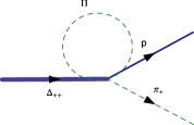
Figure 1: Next-to-the-leading hadronic decay with the adjacency of order five for the decay $\Delta_{++}\rightarrow p\pi_{+}.$

Since, the couplings of the order five adjacency (see Fig.(1)) described by the same CG coefficients as for the tree level couplings of order three adjacency, it is straightforward to program the same coupling constants for every pion field appearing in the loop. This can be easily accomplished if the field $\Pi$ is introduced in the loop. This field $\Pi$ appears only in the loops with the $3\pi$ coupling, with a propagator described as

$$\Delta_{\Pi}(q)=\sum_{i=1}^{8}\frac{1}{q^{2}-m_{i}^{2}},$$ (22)

where $m_{i}$ is the mass of the meson in the $SU\left(3\right)$ octet (see Eq.(3)). The kinematic part of the coupling for this type of processes is exactly equal to the couplings of the hadronic interactions described by chiral Lagrangians (Eqs.(1, 7 and 9)). The same is true for the CG coefficients, but with $f_{\pi}$ constant replaced by $f_{\pi}^{3}$ in the first line of Eq.(15).

IV Applications and Tests

The extension towards the hadronic sector in FeynArts and FormCalc which we propose in this work can be applied to the virtually any hadronic process. We choose two processes relevant to the problems of the hadronic physics. These are pentaquark photo-production and Compton scattering in the studies of the nucleon polarizabilities. Since these problems were addressed earlier by (Hosaka05, ) and (Meissner, ), this will serve as a test of the rather involved calculations using our Computational Hadronic Model (CHM).

IV.1 Pentaquark Photo-Production

The question of existence of exotic baryons is of crucial importance to the physics of the strong interactions. The bound states of five quarks (pentaquark) can be described by the at least two models. Nucleon-Kaon molecule model, proposed by (Diakonov97, ), assumes that pentaquark is formed by a nucleon and a kaon bounded via the nuclear strong interaction. An alternative model proposed by (Wilczek, ) treat a pentaquark as a system of two diquarks and one anti-quark $(q^{4}\overline{q})$, bounded via the colour strong interaction. Since the range of the nuclear strong interaction is of order of $\sim 1\,fm$, compared to the color strong interaction range, of $\sim 0.1\,fm$, the decay widths of the pentaquark in these two models are substantially different ($\sim 100\,MeV$ vs $\sim 1\,MeV$). Obviously, the detection and subsequent measurements of the pentaquark decay width will most probably rule out one of these models. In the experimental searches of the exotic baryons, attention goes towards lightest pentaquark state $\Theta_{5}^{+}=\{uuds\bar{s}\}$, which has a mass around $1540\,MeV$. This state is attractive not only because it has the highest production probability, but also due to the fact that symmetries of the chiral Lagrangian forbid the electromagnetic decay of this state to the proton and photon at the tree level and hence makes $\Theta_{5}^{+}$ state more stable with decay width probably around $1\,MeV$. Unfortunately, despite of tremendous experimental efforts, production of this state proved to be extremely problematic. The experimental difficulties emerge from the weak signal, low statistics, and high background in all production channels.

From the point of view of relativistic ChPT it is possible to introduce pentaquark baryons in to the computational hadronic model due to the same symmetry of the chiral Lagrangian and similarities of the $10$ and $\overline{10}$ irreducible representations of the $SU(3)$ group. If one assumes that octet of the pentaquarks is represented by the spin $1/2$ states, and the anti-decuplet of resonances by the spin $J^{P}=3/2^{\pm}$, it easy to construct a Lagrangian for both. Using notation of (Beane, ), we can describe the octet of exotic baryons by

$$\mathcal{O}_{5}=\left(\begin{array}[]{ccc}\frac{1}{\sqrt{2}}\sum_{5}^{0}+\frac{1}{\sqrt{6}}\Lambda_{5}&\sum_{5}^{+}&p_{5}\\ \sum_{5}^{-}&-\frac{1}{\sqrt{2}}\sum_{5}^{0}+\frac{1}{\sqrt{6}}\Lambda_{5}&n_{5}\\ \Xi_{5}^{-}&\Xi_{5}^{0}&-\frac{2}{\sqrt{6}}\Lambda_{5}\end{array}\right),$$ (23)

and the anti-decuplet of pentaquark resonances by

$$T_{5}^{333} =\Theta_{5}^{+},$$

$$T_{5}^{133} =\frac{1}{\sqrt{3}}N_{5}^{0},\,T_{5}^{233}=\frac{1}{\sqrt{3}}N_{5}^{+},$$

$$T_{5}^{113} =\frac{1}{\sqrt{3}}\sum\nolimits_{5}^{-},\,T_{5}^{123}=\frac{1}{\sqrt{6}}\sum\nolimits_{5}^{0},\,T_{5}^{223}=\frac{1}{\sqrt{3}}\sum\nolimits_{5}^{+},$$ (24)

$$T_{5}^{111} =\Xi_{5}^{--},\,T_{5}^{112}=\frac{1}{\sqrt{3}}\Xi_{5}^{-},\,T_{5}^{122}=\frac{1}{\sqrt{3}}\Xi_{5}^{0},\,T_{5}^{222}=\Xi_{5}^{+}.$$

The interaction Lagrangian for all the possible permutations of the fields $B,T_{\mu},\mathcal{O}_{5},T_{5,\mu}$ and $A_{\mu}$ can be written in the following form:

$$\mathfrak{L}^{(\overline{10}\oplus 8)}= 2\mathcal{D}_{\mathcal{O}}\,Tr\,\bar{\mathcal{O}}_{5}\gamma^{\mu}\gamma_{5}\left\{A_{\mu},\mathcal{O}_{5}\right\}+2\mathcal{F}_{\mathcal{O}}\,Tr\,\bar{\mathcal{O}_{5}}\gamma^{\mu}\gamma_{5}\left[A_{\mu},\mathcal{O}_{5}\right]+2\mathcal{H}_{P}\bar{T}_{5}^{\mu}\gamma^{\nu}\gamma_{5}A_{\nu}\Gamma_{5}T_{5,\mu}+$$

$$\mathcal{C}_{P\mathcal{O}}\left(\bar{\mathcal{O}_{5}}A_{\mu}\Gamma_{5}T_{5}^{\mu}+\bar{T}_{5}^{\mu}A_{\mu}\Gamma_{5}\mathcal{O}_{5}\right)+\mathcal{C}_{PB}\left(\bar{B}A_{\mu}\Gamma_{5}T_{5}^{\mu}+\bar{T}_{5}^{\mu}A_{\mu}\Gamma_{5}B\right)+$$

$$2\mathcal{D}_{\mathcal{O}B}\,\left(Tr\,\bar{\mathcal{O}}_{5}\gamma^{\mu}\gamma_{5}\left\{A_{\mu},B\right\}+h.c.\right)+2\mathcal{F}_{\mathcal{O}B}\,\left(Tr\,\bar{B}\gamma^{\mu}\gamma_{5}\left[A_{\mu},\mathcal{O}_{5}\right]+h.c.\right).$$

Relevant to the physics of the pentaquark production, coupling constant $\mathcal{C}_{PB}$ in Eq.(IV.1) is given by $\mathcal{C}_{PB}=\frac{g_{TBP}\,f_{P}}{M_{P}}$. The constant $g_{TBP}$ can be extracted from the information on hadronic decay width of the specific pentaquark state. The rest of the coupling constants can either be extracted using the Adler-Weisberger sum rules (see (Beane, )) or require additional experimental input. The Clebsh-Gordan coefficients for the pentaquark states were computed in the same way as in Eq.(15) and Eq.(16) but with coupling constants taken from Lagrangian in Eq.(IV.1).

It is natural to raise a question: if the $\Theta_{5}^{+}$ does exist, how can chiral effective theory direct experimental searches for this state? One of the possibilities would be to look at the kinematic dependencies (see (Hosaka05, )) using our Computational Hadronic Model. There are three possible channels for the production $\Theta_{5}^{+}$: photo-, hadro- and lepto-production. The most recent experimental efforts were directed to the photo-production of the $\Theta_{5}^{+}$. Photo-production is described by the two reactions, $\gamma p\rightarrow\Theta_{5}^{+}\overline{K}_{0}$ on the proton target and $\gamma n\rightarrow\Theta_{5}^{+}K_{-}$ on the neutron target. The decision to look at these two channels explicitly is motivated by controversy over experimental results (see (CLAS05, )). Our goal here is to construct the production cross sections for these two reactions and to compare our results to (Hosaka05, ). In the Born approximation diagrams, responsible for the production of $\Theta_{5}^{+}$ are given by the contact, $s$, $t$ and $u$ channels and shown on the Fig.(2).

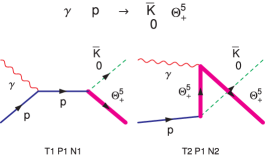
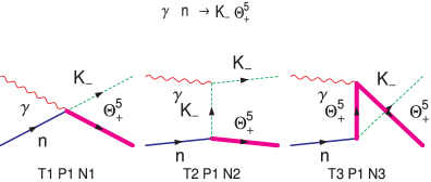
Figure 2: $\Theta_{5}^{+}$photo-production predictions from the FeynArt’s Computational Hadronic Model.

Obviously there is a distinctive asymmetry in the production channels for the two targets. This asymmetry is reflected by the presence of the contact term in photoproduction on the neutron target. This result was pointed out originally by (Hosaka05, ) and confirmed in our CHM. According to the Lagrangian given by Eq.(IV.1), we can construct two parity states of $\Theta_{5}^{+}$ with $J^{P}=3/2^{+}$or $J^{P}=3/2^{-}$ with values for the coupling constant $g_{KN\Theta}=0.53$ for $\Theta_{5}^{+}(3/2^{+})$ and $g_{KN\Theta}=4.22$ for $\Theta_{5}^{+}(3/2^{-})$ (Hosaka05, ) if we assume that this state has a narrow decay width around $1\,MeV.$ The production cross sections for the contact, $s-,$ $t-$ and $u$- channels are shown on Fig.(3) as functions of the photon’s energy $E_{\gamma}$ in the laboratory reference frame.

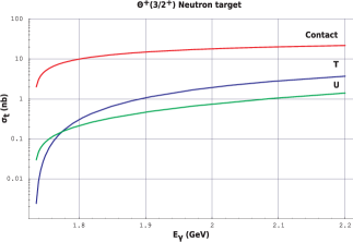
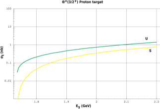
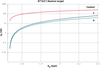
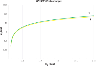
Figure 3: The total cross section for the $\Theta_{5}^{+}$ photo-production in the contact, s-, t- and u-channels as a function of energy of the photon $E_{\gamma}$ in the laboratory reference frame.

The largest contribution comes from the contact term which is only present for the neutron target. Comparing our results to (Hosaka05, ) we can see what s- and u-channel cross sections are somewhat larger in our case. This can be explained by the fact that, unlike in CHM model, the couplings in (Hosaka05, ) are adjusted by the four-dimensional formfactors, and, since in these channels baryons are further off-shell, the contribution of these channels is strongly suppressed. As for the contact and t-channel contribution, our results are close to (Hosaka05, ). The evident asymmetry between neutron and proton targets favors deuterium target (with proton as a spectator) for the photo-production of the $\Theta_{5}^{+}(3/2^{\pm})$ with production cross section around $\sim 200\,nb$ and $\sim 30\,nb$, respectively.

IV.2 Compton Scattering

Although the CHM predictions of the pentaquark photoproduction confirmed the earlier theoretical findings, our calculations are done using the Born approximation only, and hence it is reasonable to raise the question about the validity of our CHM extension of FeynArts and FormCalc for the Next-to-the-Leading-Order (NLO) calculations.

To test our NLO calculations (not including resonances) we decided to compute amplitudes for the Compton scattering off the proton and neutron. If we consider a nucleon with structure, the Compton scattering amplitude in the rest frame has the following form (Meissner, ):

$$M(\gamma N\rightarrow\gamma N)=-\frac{e^{2}Z^{2}}{4\pi m}\overrightarrow{\epsilon}^{\prime}\cdot\overrightarrow{\epsilon}+\alpha\omega^{\prime}\omega\overrightarrow{\epsilon}^{\prime}\cdot\overrightarrow{\epsilon}+\beta(\overrightarrow{\epsilon}^{\prime}\times\overrightarrow{k}^{\prime})(\overrightarrow{\epsilon}\times\overrightarrow{k})+\mathcal{O}(\omega^{4}).$$ (26)

Here, $(\overrightarrow{\epsilon},\,\omega,\,\overrightarrow{k})$ is the polarization vector, frequency and momenta of the incoming photon, respectively. Primed quantities denote the outgoing photon. Two structure constants $\alpha$ and $\beta$ are the electric and magnetic polarizabilities of the nucleon. For the point like nucleon, we have (see Fig.(4)):

$$M_{0}=-\frac{e^{2}Z^{2}}{4\pi m}\overrightarrow{\epsilon}^{\prime}\cdot\overrightarrow{\epsilon}.$$ (27)

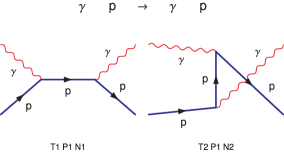
Figure 4: FeynArts output for the Compton scattering at the tree level in CHM.

This amplitude, in order to satisfy the gauge invariance of the electromagnetic current $(\partial^{\mu}J_{\mu}=0),$ is not renormalized, and expressed through the set of physical observables such as charge and mass. Moreover, in the Thomson limit when $\overrightarrow{k}^{\prime}\rightarrow\overrightarrow{k}$, the Compton amplitude $M$ in Eq.(26) should take the form of $M_{0}$ in Eq.(27) according to the well known low-energy theorem. Hence, when soft photons are considered, the nucleon behaves as a point-like particle and structure constants of Eq.(26) could be calculated only through the loop diagrams. Although generally the loop contribution is ultraviolet divergent and requires renormalization, this is not a case for the Compton scattering. If $M(\overrightarrow{k}^{\prime}\rightarrow\overrightarrow{k})\rightarrow M_{0}$, $M_{0}$ is not renormalized and the limit $\overrightarrow{k}^{\prime}\rightarrow\overrightarrow{k}$ does not remove ultraviolet divergences, then the amplitude $M$ should be finite. If we take only the $SU(2)$ triplet of the mesons, we will have to evaluate 22 diagrams for the neutron and 52 diagrams for the proton (see Fig.(5)).

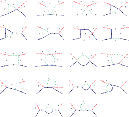
Figure 5: Representative diagrams for the Next-to-the-Leading order Compton scattering in CHM.

It is necessary to mention that the diagrams on Fig.(5) represent only generic types of the topologies allowed in Compton scattering. When one employs CHM, the full set of graphs will have to include the crossed diagrams and wave function renormalization graphs absorbed into counterterms. Also, in the CHM, charged mesons are treated as non-selfconjugate fields which effectively induce double counting, so part of the final amplitude with the charged mesons in the loops has to be divided by the factor of two.

Individually, the diagrams on Fig.(5) give the divergent contributions but their sum should be a finite result. That was a case when Compton amplitude was computed in the CHM. We observed analytically that the final Compton amplitude is, in fact, finite (i.e. free of ultraviolet divergences). Moreover, we have successfully tested finiteness of the Compton amplitude for the $SU(3)$ octet of mesons. Here we have calculated 44 graphs for the neutron and 104 (not including wave function renormalization graphs) for the proton and observed no ultraviolet divergences in the final amplitude. In the FormCalc, the final results (amplitude or Compton tensor) were presented analytically using the Passarino-Veltman basis. Due to the cumbersome nature of this type of calculations we leave analytical details out of this article. Although we can proceed and express polarizabilities of the nucleon numerically, we leave that for the next publication. We have satisfied purpose of this article already when ultraviolet finite results for the Compton amplitude were obtained up to NLO using our computational hadronic model.

V Conclusion and Outlook

In the present work we have developed an extension (the Computational Hadronic Model) of FeynArts and FormCalc to include the hadronic sector using Chiral Perturbation Theory. We have included octet of mesons, baryons (and pentaquark baryons) plus the decuplet of resonances (and the anti-decuplet of pentaquark resonances). The CHMs provides a robust prediction of the asymmetry in pentaquark $\Theta_{5}^{+}$ photoproduction between neutron and proton targets. It can be concluded that the asymmetry is caused by the presence of the contact term in the $\gamma n\rightarrow K^{-}\Theta_{5}^{+}$channel.

The ability of the CHM to handle Next-to-the-Leading-Order calculations was tested through the fact that the Compton scattering amplitude should be ultraviolet finite and should not be renormalized. As was expected, even when the entire octet of mesons was included, the final amplitude did not exhibit any ultraviolet divergent behavior. The NLO results of the CHM can be expressed analytically using FormCalc, with an amplitude expressed in the Passarino-Veltman basis as well as numerically with application of the package LoopTools.

Future applications of the CHM can be envisioned for calculations of many processes, including the full kinematic dependencies for the production/decay channels of hadronic physics. Source files of the CHM are available by request from the authors.

VI Acknowledgment

This work has been supported by both an NSERC Discovery Grant, and A. Aleksejevs is grateful for support from Saint Mary’s University through its NSERC Research Capacity Development Grant. We are grateful to S. Barkanova of Acadia University for the useful discussions. The authors would also like to acknowledge the role of the T. Hahn who made packages such as FeynArts, FormCalc and LoopTools available to physics community.

References

- (1) T. Hahn, arXiv:hep-ph/0012260v2.
- (2) T. Hahn, M. Perez-Victoria, arXiv:hep-ph/9807565v1.
- (3) FeynCalc, Comp. Phys. Comm. 64 345 (1991).
- (4) J. A. M. Vermaseren, math-ph/0010025.
- (5) A. Denner, S. Dittmaier, and T. Hahn, Phys. Rev. D56 117 (hep-ph/9612390) (1997).
- (6) A. Denner and T. Hahn, Nucl. Phys. B525 27 (hep-ph/9711302) (1998) .
- (7) W. Beenakker and A. Denner, Int. J. Mod. Phys. A9 4837 (1994) .
- (8) T. Hahn (hep-ph/0007062).
- (9) W. Hollik, C. Schappacher Nucl. Phys. B545 98 (hep-ph/9807427) (1999).
- (10) J. Guasch, W. Hollik, and A. Kraft Nucl. Phys. B596 66 (hep-ph/9911452) (2001).
- (11) A. Manohar, hep-ph/9305298 (1993).
- (12) E. Jenkins, and A. Manohar, UCSD/PTH 91-30, (1991).
- (13) M. N. Butler, M. J. Savage, and R. P. Springer, Nucl. Phys. B399, 69 (1993).
- (14) M. Benmerrouche, R. M. Davidson, and N. C. Mukhopadhyay, Phys. Rev. C39(6), 2339 (1989).
- (15) A. Denner, Fortschr. d. Physik, 41, 4 (1993).
- (16) D. Diakonov, V. Petrov, and M. Polyakov, Z. Phys. A359, 305 (1997).
- (17) R. Jaffe, and F. Wilczek, hep-ph/0307341v4 (2003).
- (18) S. Nam, A. Hosaka, and H. Kim, hep-ph/0505134v2 (2005).
- (19) R. De Vita et al., [CLAS Collaboration], talk given at APS april meeting (2005).
- (20) V. Bernard, N. Kaiser, and U.-G. Meisner, BUTP-91/30 (1991).
- (21) S. R. Beane, arXiv:hep-ph/0408066v1 (2004).