Markov Chain Methods For Analyzing Complex Transport Networks

Abstract

We have developed a steady state theory of complex transport networks used to model the flow of commodity, information, viruses, opinions, or traffic. Our approach is based on the use of the Markov chains defined on the graph representations of transport networks allowing for the effective network design, network performance evaluation, embedding, partitioning, and network fault tolerance analysis. Random walks embed graphs into Euclidean space in which distances and angles acquire a clear statistical interpretation. Being defined on the dual graph representations of transport networks random walks describe the equilibrium configurations of not random commodity flows on primary graphs. This theory unifies many network concepts into one framework and can also be elegantly extended to describe networks represented by directed graphs and multiple interacting networks.

PACS codes: 89.75.Fb, 89.75.-k, 89.90.+n

Keywords: Random walks; complex networks; traffic equilibrium.

1 Introduction

Transport networks are used to model the flow of commodity, information, viruses, opinions, or traffic. They typically represent the networks of roads, streets, pipes, aqueducts, power lines, or nearly any structure which permits either vehicular movement or flow of some commodity, products, goods or service. The major aim of the analysis is to determine the structure and properties of transport networks that are important for the emergence of complex flow patterns of vehicles (or people) through the network such as the Braess paradox [1]. This counter-intuitive phenomenon occurs when adding more resources to a transportation network (say, a new road or a bridge) deteriorates the quality of traffic by creating worse delays for the drivers, rather than alleviate it. The Braess paradox has been observed in the street vehicular traffic of New York City and Stuttgart, [2].

The paper is partitioned into three sections. In Sec. 2, we demonstrate that Markov chains arise naturally in the problem of network equilibriums. Random walks embed connected undirected graphs into Euclidean space that can be used in order to investigate them. In Sec. 3, we discuss the thermodynamics of random walks defined on the undirected graph representations of transport networks. In Sec. 4, we extend the approach to networks represented by directed graphs and to multiple interacting networks. We conclude in the last section.

2 Euclidean Space Associated to Transport Networks

The main goal of complex network theory is to study relationships between parts of complex systems that gives rise to the patterns of collective behavior and of interactions between complex systems with their environments.

2.1 Traffic equilibrium, space syntax, and random walks

Given a connected undirected graph $G(V,E)$, in which $V$ is the set of nodes and $E$ the set of edges, we introduce the traffic volume $f:E\to(0,\infty[$ through every edge $e\in E$. It then follows from the Perron-Frobenius theorem that the linear equation

$$f(e)\,=\,\sum_{e^{\prime}\,\in\,E}\,f(e^{\prime})\,\exp\left(\,-h\,\ell\left(e^{\prime}\right)\,\right)$$ (1)

has a unique positive solution $f(e)>0$, for every edge $e\in E$, for a fixed positive constant $h>0$ and a chosen set of positive metric length distances $\ell(e)>0$. This solution is naturally identified with the traffic equilibrium state of the transport network defined on $G$, in which the permeability of edges depends upon their lengths. The parameter $h$ is called the volume entropy of the graph $G$, while the volume of $G$ is defined as the sum

$$\mathrm{Vol}(G)\,=\,\frac{1}{2}\,\sum_{e\in E}\,\ell(e).$$

The volume entropy $h$ is defined to be the exponential growth of the balls in a universal covering tree for $G$ with the lifted metric, [3]-[6].

The degree of a node $v\in V$ is the number of its neighbors in $G$, $\deg(v)=k_{v}$. It has been shown in [6] that among all undirected connected graphs of normalized volume, $\mathrm{Vol}(G)=1$, which are not cycles and $k_{v}\neq 1$ for all nodes, the minimal possible value of the volume entropy, $\min(h)=\frac{1}{2}\sum_{v\in V}k_{v}\,\log\left(k_{v}-1\right)$ is attained for the length distances

$$\ell(e)\,=\,\frac{\log\left(\left(k_{i(e)}-1\right)\left(k_{t(e)}-1\right)\right)}{2\,\min(h)},$$ (2)

where $i(e)\in V$ and $t(e)\in V$ are the initial and terminal vertices of the edge $e\in E$ respectively. It is then obvious that substituting (2) and $\min(h)$ into (1) the operator $\exp\left(-h\ell(e^{\prime})\right)$ is given by a symmetric Markov transition operator,

$$f(e)\,=\,\sum_{e^{\prime}\,\in\,E}\,\frac{f(e^{\prime})}{\sqrt{\left(k_{i(e^{\prime})}-1\right)\left(k_{t(e^{\prime})}-1\right)}},$$ (3)

which rather describes time reversible random walks over edges than over nodes. In other words, we are invited to consider random walks on the dual graphs. The flows satisfying (1) with the operator (3) meet the mass conservation property, $\sum_{i\sim j}f_{ij}=\pi_{j}$, $\sum_{j\in V}\pi_{j}=1$. The Eq.(3) unveils the indispensable role Markov’s chains defined on edges play in equilibrium traffic modelling and exposes the degrees of nodes as a key determinant of the transport networks properties.

The notion of traffic equilibrium had been introduced by J.G. Wardrop in [7] and then generalized in [8] to a fundamental concept of network equilibrium. Wardrop’s traffic equilibrium is strongly tied to the human apprehension of space since it is required that all travellers have enough knowledge of the transport network they use. The human perception of places is not an entirely Euclidean one, but are rather related to the perceiving of the vista spaces (streets and squares) as single units and of the understanding of the topological relationships between these vista spaces, [9]. Decomposition of city space into a complete set of intersecting vista spaces produces a spatial network which we call the dual graph representation of a city. Therein, the relations between streets treated as nodes are traced through their junctions considered as edges.

Dual city graphs are extensively investigated within the concept of space syntax, a theory developed in the late 1970s, that seeks to reveal the mutual effects of complex spatial urban networks on society and vice versa, [10, 11]. Spatial perception that shapes peoples understanding of how a place is organized determines eventually the pattern of local movement which is predicted by the space syntax method with surprising accuracy [12].

2.2 Euclidean space of undirected graphs associated to random walks

Any graph representation naturally arises as the outcome of a categorization, when we abstract a real world system by eliminating all but one of its features and by grouping together things (or places) sharing a common attribute. All elements called nodes that fall into one and the same group $V$ are considered as essentially identical; permutations of them within the group are of no consequence. The symmetric group $\mathbb{S}_{N}$ consisting of all permutations of $N$ elements ($N$ being the cardinality of the set $V$) constitute the symmetry group of $V$. If we denote by $E\subseteq V\times V$ the set of ordered pairs of nodes called edges, then a graph is a map $G(V,E):E\to K\subseteq\mathbb{R}_{\,+}$ (we suppose that the graph has no multiple edges).

The nodes of $G(V,E)$ can be weighted with respect to some measure $m=\sum_{i\in V}m_{i}\delta_{i},$ specified by a set of positive numbers $m_{i}>0$. The space $\ell^{2}(m)$ of square-assumable functions with respect to the measure $m$ is a Hilbert space $\mathcal{H}$. Among all linear operators defined on $\mathcal{H}$, those invariant under the permutations of nodes are particularly interesting since they reflect the symmetry of the graph. Although there are infinitely many such operators, only those which maintain conservation of a quantity may describe a physical process. The Markov transition operators which share the property of probability conservation considered in the theory of random walks on graphs are among them. Another example is given by the Laplace operators satisfying the mean value property (mass conservation) [13].

Markov’s operators on Hilbert space form the natural language of complex networks theory. Being defined on connected undirected graphs, a Markov transition operator $T$ has a unique equilibrium state $\pi$ ( stationary distribution of the random walk) such that $\pi T=\pi$ and $\pi=\lim_{t\to\infty}\,\sigma\,T^{\,t}$ for any density $\sigma\in\mathcal{H}$ ($\sigma_{i}\geq 0$, $\sum_{i\in V}\sigma_{i}=1$). There is a unique measure $m_{\pi}=\sum_{i\,\in\,V}\pi_{i}\delta_{i}$ related to the stationary distribution $\pi$ with respect to which the Markov operator $T$ is self-adjoint,

$$\widehat{T}=\,\frac{1}{2}\left(\pi^{1/2}\,\,T\,\,\pi^{-1/2}+\pi^{-1/2}\,\,T^{\top}\,\,\pi^{1/2}\right),$$ (4)

where $T^{\top}$ is the adjoint operator. The orthonormal ordered set of real eigenvectors $\psi_{i}$, $i=1\ldots N$, of the symmetric operator $\widehat{T}$ defines a basis in $\mathcal{H}$. In the theory of random walks defined on graphs [15, 14] and in spectral graph theory [16], the properties of graphs are studied in connection with the eigenvalues and eigenvectors of self-adjoint operators defined on them. In particular, the symmetric transition operator of the random walk defined on undirected graphs is $\widehat{T_{ij}}=1/\sqrt{k_{i}k_{j}}$ if $i\sim j$. Its first eigenvector $\psi_{1}$ belonging to the largest eigenvalue $\mu_{1}=1$,

$$\psi_{1}\,\widehat{T}\,=\,\psi_{1},\quad\psi_{1,i}^{2}\,=\,\pi_{i},$$ (5)

describes the local property of nodes (connectivity), $\pi_{i}=k_{i}/2M,$ where $2M=\sum_{i\in V}k_{i}$, while the remaining eigenvectors $\left\{\,\psi_{s}\,\right\}_{s=2}^{N}$ belonging to the eigenvalues $1>\mu_{2}\geq\ldots\mu_{N}\geq-1$ describe the global connectedness of the graph.

Markov’s symmetric transition operator $\widehat{T}$ defines a projection of any density $\sigma\in\mathcal{H}$ on the eigenvector $\psi_{1}$ of the stationary distribution $\pi$,

$$\sigma\,\widehat{T}\,=\,\psi_{1}+\sigma^{\bot}\,\widehat{T},\quad\sigma^{\bot}\,=\,\sigma-\psi_{1},$$ (6)

in which $\sigma^{\bot}$ is the vector belonging to the orthogonal complement of $\psi_{1}$. Thus, it is clear that any two densities $\sigma,\rho\,\in\,\mathcal{H}$ differ with respect to random walks only by their dynamical components, $(\sigma-\rho)\,\widehat{T}^{t}\,=\,(\sigma^{\bot}-\rho^{\bot})\,\widehat{T}^{t}$ for all $t\,>\,0$. Therefore, we can define the distance $\|\ldots\|_{T}$ between any two densities which they acquire with respect to random walks by

$$\left\|\,\sigma-\rho\,\right\|^{2}_{T}\,=\,\sum_{t\,\geq\,0}\,\left\langle\,\sigma-\rho\,\left|\,\widehat{T}^{t}\,\right|\,\sigma-\rho\,\right\rangle.$$ (7)

or, using the spectral representation of $\widehat{T}$,

$$\left\|\,\sigma-\rho\,\right\|^{2}_{T}\,=\,\sum_{t\,\geq 0}\,\sum_{s=2}^{N}\,\mu^{t}_{s}\,\left\langle\,\sigma-\rho\,|\,\psi_{s}\right\rangle\!\left\langle\,\psi_{s}\,|\,\sigma-\rho\,\right\rangle\,=\,\sum_{s=2}^{N}\,\frac{\left\langle\,\sigma-\rho\,|\,\psi_{s}\right\rangle\!\left\langle\,\psi_{s}\,|\,\sigma-\rho\,\right\rangle}{\,1\,-\,\mu_{s}\,},$$ (8)

where we have used Dirac s bra-ket notations especially convenient in working with inner products and rank-one operators in Hilbert space.

If we introduce in $\mathcal{H}(V)$ a new inner product by

$$\left(\,\sigma,\rho\,\right)_{T}\,=\,\sum_{t\,\geq\,0}\,\sum_{s=2}^{N}\,\frac{\,\left\langle\,\sigma\,|\,\psi_{s}\,\right\rangle\!\left\langle\,\psi_{s}\,|\,\rho\right\rangle}{\,1\,-\,\mu_{s}\,}$$ (9)

for all $\sigma,\rho\,\in\,\mathcal{H}(V),$ then (8) is nothing else but

$$\left\|\,\sigma-\rho\,\right\|^{2}_{T}\,=\left\|\,\sigma\,\right\|^{2}_{T}+\left\|\,\rho\,\right\|^{2}_{T}-2\left(\,\sigma,\rho\,\right)_{T},$$ (10)

where

$$\left\|\,\sigma\,\right\|^{2}_{T}\,=\,\,\sum_{s=2}^{N}\,\frac{\left\langle\,\sigma\,|\,\psi_{s}\,\right\rangle\!\left\langle\,\psi_{s}\,|\,\sigma\,\right\rangle}{\,1\,-\,\mu_{s}\,}$$ (11)

is the square of the norm of $\sigma\,\in\,\mathcal{H}(V)$ with respect to random walks. We finish the description of the $(N-1)$-dimensional Euclidean space structure of $G$ induced by random walks by mentioning that given two densities $\sigma,\rho\,\in\,\mathcal{H}(V),$ the angle between them can be introduced in the standard way,

$$\cos\,\angle\left(\rho,\sigma\right)=\frac{\,\left(\,\sigma,\rho\,\right)_{T}\,}{\left\|\,\sigma\,\right\|_{T}\,\left\|\,\rho\,\right\|_{T}}.$$ (12)

Random walks embed connected undirected graphs into Euclidean space. This embedding can be used in order to compare nodes and to retrace the optimal coarse-graining representations. Namely, let us consider the density $\delta_{i}$ which equals 1 at the node $i\,\in\,V$ and zero for all other nodes. With respect to the measure $m_{\pi}$, it corresponds to the density $\upsilon_{i}\,=\,\pi^{-1/2}_{i}\,\delta_{i}$. Then, the square of the norm of $\upsilon_{i}$ is given by

$$\left\|\,\upsilon_{i}\,\right\|_{T}^{2}\,=\,{\frac{1}{\pi_{i}}\,\sum_{s=2}^{N}\,\frac{\,\psi^{2}_{s,i}\,}{\,1-\mu_{s}\,}},$$ (13)

where $\psi_{s,i}$ is the $i^{\mathrm{th}}$-component of the eigenvector $\psi_{s}$. In the theory of random walks [15], the quantity (13) expresses the access time to a target node quantifying the expected number of steps required for a random walker to reach the node $i\in V$ starting from an arbitrary node chosen randomly among all other nodes with respect to the stationary distribution $\pi$.

The Euclidean distance between any two nodes of the graph $G$ induced by random walks,

$$K_{i,j}\,=\,\left\|\,\upsilon_{i}-\upsilon_{j}\,\right\|^{2}_{T},$$ (14)

is simply the commute times in theory of random walks and is equal to the expected number of steps required for a random walker starting at $i\,\in\,V$ to visit $j\,\in\,V$ and then to return to $i$ again, [15].

It is important to mention that the cosine of an angle calculated in accordance to (12) has the structure of Pearson’s coefficient of linear correlations that reveals it’s natural statistical interpretation. Correlation properties of flows of random walkers passing by different paths have been remained beyond the scope of previous studies devoted to complex networks and random walks on graphs. The notion of angle between any two nodes in the graph arises naturally as soon as we become interested in the strength and direction of a linear relationship between two random variables, the flows of random walks moving through them. If the cosine of an angle (12) is 1 (zero angles), there is an increasing linear relationship between the flows of random walks through both nodes. Otherwise, if it is close to -1 ($\pi$ angle), there is a decreasing linear relationship. The correlation is 0 ($\pi/2$ angle) if the variables are linearly independent. It is important to mention that as usual the correlation between nodes does not necessary imply a direct causal relationship (an immediate connection) between them.

2.3 Graph partitioning by random walks

Visual segmentation of networks based on 3D representations of their dual graphs is not always feasible. The graph partitioning problem seeks to partition a weighted undirected graph $G$ into $n$ weakly connected components $\Gamma_{1},\ldots\Gamma_{n}$ such that $\bigcup_{i=1}^{n}\Gamma_{n}\subset G$ and either their properties share some common trait or the graphs nodes belonging to them are close to each other according to some distance measure defined on nodes of the graph. A number of different graph partitioning strategies for undirected weighted graphs have been studied in connection with object recognition and learning in computer vision [17]. In statistics, Principal Component Analysis (PCA) is used for the reducing size of a data set. It is achieved by the optimal linear transformation retaining the subspace that has largest variance (a lower-order principal component) and ignoring higher-order ones [18, 19].

Given an operator $S$ self-adjoint with respect to the measure $m$ defined on a connected undirected graph $G$, it is well known that the eigenvectors of the symmetric matrix ${\bf S}$ form an ordered orthonormal basis $\left\{\phi_{k}\right\}$ with real eigenvalues $\mu_{1}\geq\ldots\geq\mu_{N}$. The ordered orthogonal basis represents the directions of the variances of variables described by $S$. The number of components which may be detected in a network with regard to a certain dynamical process defined on it depends upon the number of essential eigenvectors of $S$.

Let us consider the normalized Laplace operator, [16],

$$\widehat{L_{ij}}\,=\,\delta_{ij}-\widehat{T_{ij}},$$ (15)

where $\widehat{T_{ij}}$ is the symmetric Markov transition operator $\widehat{T_{ij}}$. Its eigenvalues,

$$0\,=\,\lambda_{1}\,<\,\ldots\,\leq\,\lambda_{n}\,\leq\,\tau^{\,-1}\,<\,\ldots\,\leq\,\lambda_{N}\,\leq\,2,$$ (16)

can be interpreted as the inverse characteristic time scales of the diffusion process such that the smallest eigenvalues correspond to the stationary distribution $\pi$ together with the slowest diffusion modes involving the most significant amounts of flowing commodity.

There is a simple time scale argument which we use in order to determine the number of applicable eigenvectors from the ordered orthogonal basis of eigenvectors, $\left[\,{\bf f}_{1},\ldots{\bf f}_{N}\,\right]$. It is obvious that while observing the network close to an equilibrium state during short time, we detect flows resulting from a large number of transient processes evolving toward the stationary distribution and being characterized by the relaxation times $\propto\lambda^{-1}_{k}$. While measuring the flows in sufficiently long time $\tau$, we may discover just $n$ different eigenmodes (16). In general, the longer is the time of measurements $\tau$, the less is the number of eigenvectors we have to take into account in network component analysis of the network. Should the time of measurements be fixed, we can determine the number $n$ of required eigenvectors.

In order to obtain the best quality segmentation, it is convenient to center the $n$ primary eigenvectors. The centroid vector (representing the center of mass of the set $\left[\,{\bf f}_{1},\ldots{\bf f}_{n}\,\right]$) is calculated as the arithmetic mean,

$${\bf m}\,=\,\frac{1}{n}\,\sum_{k=1}^{n}\,{\bf f}_{k}.$$ (17)

Let us denote the $n\,\times\,N$ matrix of $n$ centered eigenvectors by

$${\bf F}\,=\,\left[\,{\bf f}_{1}\,-\,{\bf m},\ldots\,{\bf f}_{N}\,-\,{\bf m}\right].$$

Then, the symmetric matrix of covariances between the entries of eigenvectors $\{{\bf f}_{k}\}$ is the product of ${\bf F}$ and its adjoint ${\bf F}^{\top}$,

$$\mathrm{\bf Cov}\,=\,\frac{\,\,{\bf F}\,{\bf F}^{\top}\,}{N\,-\,1}$$ (18)

It is important to note that the correspondent Gram matrix ${\bf F}^{\top}\,{\bf F}\,/(N-1)\,\equiv\,{\bf 1}$ due to the orthogonality of the basis eigenvectors. The main contributions in the symmetric matrix $\mathrm{\bf Cov}$ are related to the groups of nodes

$$\mathrm{\bf Cov}{\ }{\bf u}_{k}\,=\,\sigma_{k}\,{\bf u}_{k},$$ (19)

which can be identified by means of the eigenvectors $\{\,{\bf u}_{k}\,\}$ associated to the first largest eigenvalues among $\sigma_{1}\,\geq\,\sigma_{2},$ $\dots,\,\geq\,\sigma_{N}$. By ordering the eigenvectors in decreasing order (largest first), we generate an ordered orthogonal basis with the first eigenvector having the direction of largest variance of the components of $n$ eigenvectors $\{{\bf f}_{k}\}$. Let us note that due to the structure of ${\bf F}$ only the first $n-1$ eigenvalues $\sigma_{k}$ are not trivial. In accordance to the standard PCA notation, the eigenvectors of the covariance matrix ${\bf u}_{k}$ are called the principal directions of the network with respect to the diffusion process defined by the operator $S$. A low dimensional representation of the network is given by its principal directions $\left[\,{\bf u}_{1},\ldots,{\bf u}_{n-1}\,\right],$ for $n\,<\,N$.

Diagonal elements of the matrix $\mathrm{\bf Cov}$ quantify the component variances of the eigenvectors $\left[\,{\bf f}_{1},\ldots{\bf f}_{n}\,\right]$ around their mean values (17) and may be large essentially for large networks. Therefore, it is practical for us to use the standardized correlation matrix,

$${\mathrm{C}orr}_{ij}\,=\,\frac{\mathrm{Cov}_{ij}}{\sqrt{\mathrm{Cov}_{ii}}\sqrt{\mathrm{Cov}_{jj}}},$$ (20)

instead of the covariance matrix ${\mathrm{\bf Cov}}$. We emphasize that the diagonal elements of (20) equal 1, while the off-diagonal elements are the Pearson’s coefficients of linear correlations, [20].

Let ${\bf U}$ be the orthonormal matrix which contains the eigenvectors $\{{\bf u}_{k}\}$, $k\,=\,1,\ldots,\,n-1,$ of the covariance (or correlation) matrix as the row vectors. These vectors form the orthogonal basis of the $(n-1)$-dimensional vector space, in which every variance $({\bf f}_{k}-{\bf m})$ is represented by a point ${\bf g}_{k}\,\in\,\mathbb{R}^{\,(n-1)}$,

$${\bf g}_{k}\,=\,{\bf U}\,({\bf f}_{k}-{\bf m}\,).$$ (21)

Then each original eigenvector ${\bf f}_{k}$ can be obtained from ${\bf g}_{k}\,\in\,\mathbb{R}^{\,(n-1)}$ by the inverse transformation,

$${\bf f}_{k}\,=\,{\bf U}^{\top}\,{\bf g}_{k}\,+\,{\bf m}.$$ (22)

Using transformations (21) and (22) we obtain the $(n-1)$-dimensional representation $\left\{\,\varphi_{k}\,\right\}_{\,k=1}^{\,(n-1)}$ of the $N$-dimensional basis vectors $\left\{\,{\bf f}_{s}\,\right\}_{\,s=1}^{\,N}$ in the form

$$\varphi_{\,k}\,=\,{\bf U}^{\top}{\bf U}\,{\bf f}_{k}\,+\,\left(\,{\bf 1}-{\bf U}^{\top}{\bf U}\,\right)\,{\bf m},$$ (23)

that minimizes the mean-square error between ${\bf f}_{k}\,\in\,\mathbb{R}^{\,N}$ and $\varphi_{k}\,\in\,\mathbb{R}^{\,(n-1)}$ for given $n$.

Variances of eigenvectors $\left\{\,{\bf f}_{k}\,\right\}$ are positively correlated within a principal component of the transport network. Thus, the transition matrix ${\bf U}^{\top}{\bf U}$ can be interpreted as the connectivity patterns acquired by the network with respect to the diffusion process. Two nodes, $i$ and $j$, belong to one and the same principal component of the network if $\left({\bf U}{\bf U}^{\top}\right)_{ij}\,>\,0$. By applying the Heaviside function, which is zero for negative argument and one for positive argument, to the elements of the transition matrix ${\bf U}{\bf U}^{\top}$, we derive the coarse-grained connectivity matrix of network components.

3 Thermodynamics of Transport Networks

In the present section, we study the spectrum (16) of the normalized Laplace operator (15) defined on a connected, undirected graph $G$ by means of spectral methods strongly inspired by statistical mechanics. The obvious advantage of statistical mechanics is that statistical moments of random walks would acquire a ”physical interpretation” in the framework of this thermodynamic formalism. The full description of transport networks in short time and small scales requires a high dimensional space, e.g. the knowledge of locations and velocities of all agents participating in transport processes. Being defined on a graph, the time evolution of such a system can be described by just a few dynamically relevant variables called reaction coordinates [21]. Identification of slow variables and dynamically meaningful reaction coordinates that capture the long time evolution of transport systems is among the most important problems of transport network analysis. The spectrum of Laplace operator could have gaps indicating the time scales separation, that is, there are only a few ”slow” time scales at which the transport network is meta-stable, with many ”fast” modes describing the transient processes toward the slow modes. The methods of spectral graph theory allow detecting and separating ”slow” and ”fast” time scales giving rise to the component analysis of networks in which the primary eigenvalues play the essential role.

3.1 Spectral function of Laplace operator

Since the spectra of self-adjoint Laplace operators defined on the undirected graphs are non-negative they can be investigated by means of the characteristic functions which discriminate contributions from the largest eigenvalues of Laplace operator in favor of those from the minimal ones. These characteristic functions are usually associated with kernels.

Given a self-adjoint operator $L$ defined on a finite dimensional Hilbert space $\mathcal{H}$ the latter has an orthonormal basis $\{\phi_{k}\}_{k=1}^{N}$ and every element of the Hilbert space can be written in a unique way as a sum of multiples of these basis elements. The use of Borel’s functional calculus for a positive semi-definite operator function $f(L)$ allows us to define a Hilbert space $\mathcal{H}$ on $\mathbb{R}^{N}$ via the dot product,

$$\left\langle\phi,\phi\right\rangle_{\mathcal{H}}=\left\langle\phi,f(L)\phi\right\rangle,$$ (24)

with the kernel $f^{-1}(L)$. The kernels associated with the Laplace operator defined on an undirected graph $G$ play the role of the Green functions describing long-range interactions between different diffusion modes induced by the graph structure (the main graph components). The Green function recently introduced in [22] is specified by the parameter $\beta>0$,

$$\left({\bf K}_{\beta}\right)_{ij}=\exp(-\beta L_{i,j}),$$ (25)

and solve the diffusion equation defined on a connected, undirected graph $G$:

$$\mathcal{G}=\int_{0}^{\infty}{\bf K}_{\beta}{\ }d\beta=\int_{0}^{\infty}\exp(-\beta{\bf L}){\ }d\beta={\bf L}^{-1},$$ (26)

with initial conditions being a source at node $i\in V$ at $\beta=0$ [23]. The function $\left({\bf K}_{\beta}\right)_{ij}$ describes the expected number of particles that would accumulate at vertex $j$ after a given amount of time if they have been injected at vertex $i$ and diffused through the graph along the edges. The exponential diffusion kernel (25) discriminate large eigenvalues that is preferable while performing estimation on the graph since it biases the estimate towards functions which vary little over the graph components [24]-[25].

The distribution of eigenvalues $\lambda_{k}\in[0,2[$ of the self-adjoint Laplace operator (15) defined on the undirected graph $G$ are characterized by the spectral density function,

$$\rho(\lambda)=\sum_{k=1}^{N}\delta(\lambda-\lambda_{k}).$$ (27)

However, it is more convenient to study the properties of non-negative spectra by means of the characteristic functions.

The first characteristic function is given by the Laplace transform of the spectral density (27),

$$\begin{array}[]{lcl}Z(\beta)&=&\int_{0}^{\infty}e^{-\beta\lambda}\rho(\lambda){\ }d\lambda\\ &=&\sum_{k=1}^{N}e^{-\beta\lambda_{k}},\end{array}$$ (28)

known as the canonical partition function. encoding the statistical properties of the system being in the thermodynamic equilibrium. The inverse temperature parameter $\beta>0$ which can be considered either as an effective time scale in the problem (the number of spaces in the dual graph a walker passes through in one time step) or as the laziness parameter.

3.2 Thermodynamics of urban networks

Statistical mechanics provides a framework for relating the microscopic properties of a system to its macroscopic or bulk properties. The statistical properties of diffusions defined on undirected graphs can be described by means of canonical partition function (28), in which $\beta^{-1}$ plays the role of the inverse temperature. In statistical mechanics, the temperature arises from the fact that the system is in the thermal equilibrium with its environment that is achieved when two systems in thermal contact with each other cease to exchange energy by heat [26]. Equilibrium implies a state of balance and can be naturally interpreted as the stationary distribution $\pi$ in the framework of random walks defined on the undirected graphs.

Bringing up the concept of the canonical ensemble it is possible to derive the probability $P_{i}$ that random walkers will be in a certain ”microstate” characterized by the spectral value $\lambda_{i}$:

$$P_{i}=Z^{-1}(\beta)\exp(-\beta\lambda_{i}).$$ (29)

Therefore, the partition function (28) can be used to find the expected value of any microscopic properties of flows of the random walkers, which can then be related to some macroscopic variables related to the entire system. It is worth to mention that since random walkers neither have masses nor kinetic energy, the nontrivial macroscopic variables that can be derived from the partition function (28) characterize the the certain structural properties of the graph with respect to the self-adjoint operator defined on it.

We have discussed the thermodynamic potentials pertinent to space syntax in five different compact urban patterns in [27]. Two of them are situated on islands: Manhattan (with an almost regular grid-like city plan) and the network of Venice canals (Venice stretches across 122 small islands, and the canals serve the function of roads). We have also considered two organic cities founded shortly after the Crusades and developed within the medieval fortresses: Rothenburg ob der Tauber (the medieval Bavarian city preserving its original structure from the 13^th century) and the downtown of Bielefeld (Altstadt Bielefeld), an economic and cultural center of Eastern Westphalia. To supplement the study of urban canal networks, we have investigated that one in the city of Amsterdam. We do not reproduce the results reported in [27] in the present paper refereing interested readers to [27] for details. Below, we just give an outline of the approach and study the thermodynamic parameters which have not been investigated in our previous work.

The expected value of the ”microscopic energy” (the averaged eigenvalue) held at constant temperature $\beta^{-1}$,

$$\langle\lambda\rangle\equiv U=\frac{1}{Z(\beta)}\sum_{i=1}^{N}\lambda_{i}e^{-\beta\lambda_{i}}=-\frac{\partial_{\beta}Z(\beta)}{Z(\beta)}=-\partial_{\beta}\ln Z(\beta),$$ (30)

can be interpreted as the microscopic definition of the thermodynamic variable corresponding to the internal energy in statistical mechanics. Due to the complicated topology of streets and canals, the flows of random walkers exhibit spectral properties similar to that of a thermodynamic system characterized by a nontrivial internal energy (see Fig. 1).

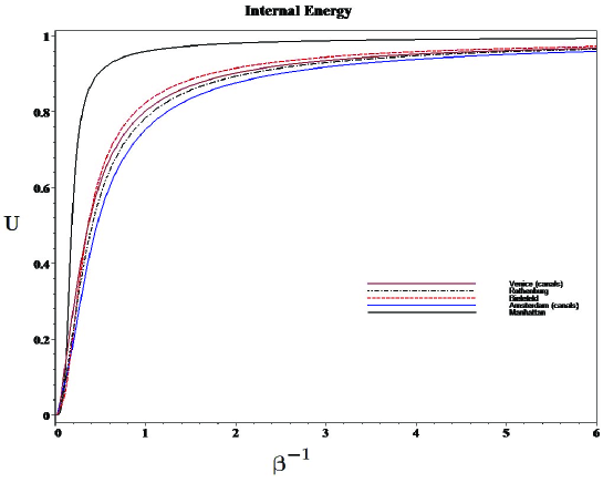
Figure 1: The expected values of the ”microscopic energy” (the averaged eigenvalues) are calculated for the spectra of compact urban patterns. The slopes of internal energy curve for the highly regular street grid of Manhattan is steeper than those for the street patterns of the organic cities (Bielefeld, Rothenburg, canals of Amsterdam and Venice).

In Fig. 1, one can clearly see the difference between the street patterns of the organic cities (Bielefeld, Rothenburg, canals of Amsterdam and Venice) and the street grid of Manhattan. Taking the derivative of $\langle\lambda\rangle$ with respect to the parameter $\beta$ in (30), we have

$$\frac{d\langle\lambda\rangle}{d\beta}=\frac{1}{Z^{2}(\beta)}\left(\frac{dZ(\beta)}{d\beta}\right)^{2}-\frac{1}{Z(\beta)}\left(\frac{d^{2}Z(\beta)}{d\beta^{2}}\right)=\langle\lambda\rangle^{2}-\langle\lambda^{2}\rangle=-D^{2}(\lambda),$$ (31)

where $D^{2}(\lambda)$ is the variance, the measure of its statistical dispersion, indicating how the eigenvalues of the normalized Laplace operator are spread around the expected value $U$ indicating the variability of the eigenvalues. The standard form of the usual deviations from the mean is the standard deviation,

$$\sigma=\sqrt{D^{2}(\lambda)}.$$ (32)

A large standard deviation indicates that the data points are far from the mean and a small standard deviation indicates that they are clustered closely around the mean (see Fig. 2).

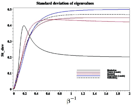
Figure 2: The deviations of eigenvalues around the ”microscopic energy” (the averaged eigenvalues) are calculated for the spectra of compact urban patterns.

In thermodynamics, heat capacity is the rate of change of temperature as heat is added to a body at the given conditions and state of the body (foremost its temperature). Similarly to pressure, it is an extensive quantity being sensitive to the network size. Dividing heat capacity by the network size yields a specific heat capacity, which is an intensive quantity that is no longer dependent on $N$, and is now dependent on the graph structure,

$${\mathcal{C}}=\frac{1}{N}\left(\frac{\partial U}{\partial T}\right)$$ (33)

We have presented the specific heat capacity, as a function of temperature in the model of random walks defined on the different compact cities in Fig. 3.

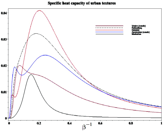
Figure 3: The specific heat capacity, as a function of temperature in the model of random walks defined on the different urban textures.

Note that the specific heat capacity is zero at zero temperature ($\beta\to\infty$), and rises to a maximal value as temperature grows up. It is interesting to note that the specific heat capacity in the random walks models defined on networks is dramatically different from that of most physical systems (like the multi-atomic gases or a crystalline solid phase); it is not a monotonous increasing function approaching the Dulong-Petit limit at higher temperature (the theoretical maximum of heat capacity). The decay of specific heat at high temperatures ($\beta\to 0$) results from the ”freezing out” of some degrees of freedom as $\beta\to 0$ (when random walkers rest at nodes most of the time).

The maximal values of the specific heat capacity is an individual characteristics of a city structure. They are higher for the organic cities and lower for those planned in a regular grid.

4 Directed and Interacting Transport Networks

Many transport networks correspond to directed graphs. Power grids transporting electrical currents and driving directions assigned to city streets in order to optimize traffic in a city are the examples [28]. Traffic within large cities is formally organized with marked driving directions creating one-way streets. On those streets all traffic must flow in only one direction, but pedestrians on the sidewalks are generally not limited to one-way movement. It is well known that the use of one-way streets would greatly improve traffic flow since the speed of traffic is increased and intersections are simplified.

Moreover, even if the network of city itineraries constitutes an undirected graph, there is a general principle that establishes who has the right to go first while crossing the road intersections or other conflicting parts of the road and who has to wait until the other driver does so. While assigning weights estimating traffic loading of itineraries on such a city graph, we could shortly discover that each road side should be characterized by its own weight depending upon the number of right-hand junctions the road has with other itineraries that is a directed weighted graph.

The spectral approach for directed graphs has not been as well developed as for undirected graph. Indeed, it is rather difficult if ever possible to define a unique self-adjoint operator on directed graphs. In general, any node $i$ in a directed graph $\vec{G}$ can have different number of in-neighbors and out-neighbors,

$$k_{\mathrm{in}}(i)\,\neq\,k_{\mathrm{out}}(i).$$ (34)

In particular, a node $i$ is a source if $k_{\mathrm{in}}(i)=0,$ $k_{\mathrm{out}}(i)\neq 0$, and is a sink if $k_{\mathrm{out}}(i)=0$, $k_{\mathrm{in}}(i)\neq 0$. If the graph has neither sources nor sinks, it is called strongly connected.

Despite asymmetric interactions represented by directed graphs are ubiquitous in many technological networks, they have not been yet very well studied in complex network theory. In general, the local structure of directed graphs is fundamentally different from that of undirected graphs. In particular, the diameters of directed networks can essentially exceeds that the one corresponding to the same networks regarded as undirected. A recent investigation into the local structure of directed networks [29] shows that directed networks often have very few short loops as compared to random models usual in contemporary theory of complex systems. In undirected networks, the high density of short loops (high clustering coefficient) together with small graph diameter gives rise to the small-world effect [30]. In directed networks, the correlation between number of incoming and outgoing edges modulates the expected number of short loops. In particular, it has been demonstrated in [29] that if the values $k_{\mathrm{in}}(i)$ and $k_{\mathrm{out}}(i)$ are not correlated, then the number of short loops is strongly reduced as compared to the case when both degrees are positively correlated.

4.1 Random walks on directed graphs

Finite random walks are defined on a strongly connected directed graph $\vec{G}(V,\vec{E})$ as finite vertex sequences $\mathfrak{w}=\{v_{0},\ldots,v_{n}\}$ (time forward) and $\mathfrak{w}^{\prime}=\{v_{-n},\ldots,v_{0}\}$ (time backward) such that each pair $(v_{i-1},v_{i})$ of vertices adjacent either in $\mathfrak{w}$ or in $\mathfrak{w}^{\prime}$ constitutes a directed edge $v_{i-1}\to v_{i}$ in $\vec{G}$.

A time forward random walk is defined by the transition probability matrix [31] $P_{ij}$ for each pair of nodes $i,j\in\vec{G}$ by

$$P_{ij}=\left\{\begin{array}[]{ll}1/k_{\mathrm{out}(i)},&i\to j,\\ 0,&\mathrm{otherwise},\end{array}\right.$$ (35)

which satisfies the probability conservation property:

$$\sum_{j,{\ }i\to j}P_{ij}=1.$$ (36)

The definition (35) can be naturally extended for weighted graphs [31] with $w_{ij}>0$,

$$P_{ij}=\frac{w_{ij}}{\sum_{s\in V}w_{is}}.$$ (37)

Matrices (35) and (37) are real, but not symmetric and therefore have complex conjugated pairs of eigenvalues. For each pair of nodes $i,j\in\vec{G}$, the forward transition probability is given by $p^{(t)}_{ij}=({\bf P}^{t})_{ij}$ that is equal zero, if $\vec{G}$ does not contain a directed path from $i$ to $j$.

Backwards time random walks are defined on the strongly connected directed graph $\vec{G}$ by the stochastic transition matrix

$${P}^{\star}_{ij}=\left\{\begin{array}[]{ll}1/k_{\mathrm{in}}(i),&j\to i,\\ 0,&\mathrm{otherwise},\end{array}\right.$$ (38)

satisfying another probability conservation property

$$\sum_{i,{\ }i\to j}P^{\star}_{ij}=1.$$ (39)

It describes random walks unfolding backwards in time: should a random walker arrives at $t=0$ at a node $v_{0}$, then

$$p^{(-t)}_{ij}=(({\bf P^{\star}})^{t})_{ij}$$ (40)

defines the probability that $t$ steps before it had originated from a node $j$. The matrix element (40) is zero, provided there is no directed path from $j$ to $i$ in $\vec{G}$.

If $\vec{G}$ is strongly connected and aperiodic, the random walk converges [32, 31, 33, 34] to the only stationary distribution $\pi$ given by the Perron vector, $\pi{\bf P}=\pi.$ If the graph $\vec{G}$ is periodic, then the transition probability matrix ${\bf P}$ can have more than one eigenvalue with absolute value 1, [16]. The components of Perron’s vector $\pi$ can be normalized in such a way that $\sum_{i}\pi_{i}=1$. The Perron vector for random walks defined on a strongly connected directed graph can have coordinates with exponentially small values, [31].

Given an aperiodic strongly connected graph $\vec{G}$, a self-adjoint Laplace operator $L=L^{\top}$ can be defined [31] as

$$L_{ij}\,=\,\delta_{ij}-\frac{1}{2}\,\left(\pi^{1/2}{\bf P}\pi^{-1/2}+\pi^{-1/2}{\bf P}^{\top}\pi^{1/2}\right)_{ij},$$ (41)

where $\pi$ is a diagonal matrix with entries $\pi_{i}$. The matrix (41) is symmetric and has real non-negative eigenvalues $0=\lambda_{1}<\lambda_{2}\leq\ldots\leq\lambda_{N}$ and real eigenvectors.

It can be easily proven [35] that the Laplace operator (41) defined on the aperiodic strongly connected graph $\vec{G}$ is equivalent to the Laplace operator defined on a symmetric undirected weighted graph $G_{w}$ on the same vertex set with weights defined by

$$w_{ij}\,=\pi_{i}P_{ij}+\pi_{j}P_{ji}.$$ (42)

4.2 Bi-orthogonal decomposition of random walks defined on strongly connected directed graphs

In order to define the self-adjoint Laplace operator (41) on aperiodic strongly connected directed graphs, we have to know the stationary distributions of random walkers $\pi$. Even if $\pi$ exists for a given directed graph $\vec{G}$, it can be evaluated usually only numerically in polynomial time [32]. Stationary distributions on aperiodic general directed graphs are not so easy to describe since they are typically non-local in sense that each coordinate $\pi_{i}$ would depend upon the entire subgraph (the number of spanning arborescences of $\vec{G}$ rooted at $i$ [32]), but not on the local connectivity property of a node itself like it was in undirected graphs. Furthermore, if the greatest common divisor of its cycle lengths in $\vec{G}$ exceeds 1, then the transition probability matrices (35) and (38) can have several eigenvectors belonging to the largest eigenvalue 1, so that the definition (41) of Laplace operator seems to be questionable.

Given a strongly connected directed graph $\vec{G}$ specified by the adjacency matrix ${\bf A}_{\vec{G}}$ $\neq{\bf A}^{\top}_{\vec{G}}$, we consider two random walks operators. A first transition operator represented by the matrix

$${\bf P}={\bf D}_{\mathrm{out}}^{-1}{\bf A}_{\vec{G}},$$ (43)

in which ${\bf D}_{\mathrm{out}}$ is a diagonal matrix with entries $k_{\mathrm{out}}(i)$, describes the time forward random walks of the nearest neighbor type defined on $\vec{G}$. Given a time forward vertex sequence $\mathfrak{w}$ rooted at $i\in\vec{G}$, the matrix element $P_{ij}$ gives the probability that $j\in\vec{G}$ is the vertex next to $i$ in $\mathfrak{w}$. A second transition operator, ${\bf P}^{\star}$, is dynamically conjugated to (43),

$$\begin{array}[]{lcl}{\bf P}^{\star}&=&{\bf D}_{\mathrm{in}}^{-1}{\bf A}^{\top}_{\vec{G}}\\ &=&{\bf D}_{\mathrm{in}}^{-1}{\bf P}^{\top}{\bf D}_{\mathrm{out}},\end{array}$$ (44)

where ${\bf D}_{\mathrm{in}}$ is a diagonal matrix with entries $k_{\mathrm{in}}(i)$. The transition operator (44) describes random walks over time backward vertex sequences $\mathfrak{w}^{\prime}$.

It is worth to mention that on undirected graphs ${\bf P}^{\star}\equiv{\bf P}$, since $k_{\mathrm{in}}(i)=k_{\mathrm{out}}(i)$ for $\forall i\in\vec{G}$ and ${\bf A}_{G}={\bf A}^{\top}_{G}.$ While on directed graphs, ${\bf P}^{\star}$ is related to ${\bf P}$ by the transformation

$${\bf P}={\bf D}_{\mathrm{out}}^{-1}\left({\bf P}^{\star}\right)^{\top}{\bf D}_{\mathrm{in}},$$ (45)

so that these operators are not adjoint, in general ${\bf P}^{\top}\neq{\bf P}^{\star}.$

We can define two different measures

$$\mu_{+}=\sum_{j}\deg_{\mathrm{out}}(j)\delta(j),\quad\mu_{-}=\sum_{j}\deg_{\mathrm{in}}(j)\delta(j)$$ (46)

associated with the out- and in-degrees of nodes of the directed graph. In accordance to (46), we define two Hilbert spaces $\mathcal{H}_{+}$ and $\mathcal{H}_{-}$ corresponding to the spaces of square summable functions, $\ell^{2}\left(\mu_{+}\right)$ and $\ell^{2}\left(\mu_{-}\right)$, by setting the norms as

$$\|x\|_{\mathcal{H}_{\pm}}=\sqrt{\left\langle x,x\right\rangle}_{\mathcal{H}_{\pm}},$$

where $\left\langle\cdot,\cdot\right\rangle_{\mathcal{H}_{\pm}}$ denotes the inner products with respect to measures (46). Then a function $f(j)$ defined on the set of graph vertices is $f_{\mathcal{H}_{-}}(j)\in\mathcal{H}_{-}$ if transformed by

$$f_{\mathcal{H}_{-}}(j)\to J_{-}f(j)\equiv\mu_{-}{}_{j}^{-1/2}f(j)$$ (47)

and $f_{\mathcal{H}_{+}}(j)\in\mathcal{H}_{+}$ while being transformed accordingly to

$$f_{\mathcal{H}_{+}}(j)\to J_{+}f(j)\equiv\mu_{+}{}_{j}^{-1/2}f(j).$$ (48)

The obvious advantage of the measures (46) against the natural counting measure $\mu_{0}=\sum_{i\in V}\delta_{i}$ is that the matrices of the transition operators $P$ and $P^{\star}$ are transformed under the change of measures as

$$P_{\mu}=J_{+}^{-1}PJ_{-},\quad P^{\star}_{\mu}=J_{-}^{-1}P^{\star}J_{+},$$ (49)

and become adjoint,

$$\begin{array}[]{l}\left(P_{\mu}\right)_{ij}=\frac{A_{\vec{G}}{}_{ij}}{\sqrt{k_{\mathrm{out}}(i)}\sqrt{k_{\mathrm{in}}(j)}},\\ \left(P^{\star}_{\mu}\right)_{ij}\equiv\left(P^{\top}_{\mu}\right)_{ij}=\frac{A^{\top}_{\vec{G}}{}_{ij}}{\sqrt{k_{\mathrm{in}}(i)}\sqrt{k_{\mathrm{out}}(j)}}.\end{array}$$ (50)

It is also important to note that

$$P_{\mu}:\mathcal{H}_{-}\to\mathcal{H}_{+}\quad\mathrm{and}\quad P^{\star}_{\mu}:\mathcal{H}_{+}\to\mathcal{H}_{-}.$$

We obtain the singular value dyadic expansion (biorthogonal decomposition introduced in [36, 37]) for the transition operator:

$${\bf P}_{\mu}=\sum_{s=1}^{N}\Lambda_{s}\varphi_{si}\psi_{si}\equiv\sum_{s=1}^{N}\Lambda_{s}\left|\varphi_{s}\rangle\langle\psi_{s}\right|,$$ (51)

where $0\leq\Lambda_{1}\leq\ldots\Lambda_{N}$ and the functions $\varphi_{k}\in\mathcal{H}_{+}$ and $\psi_{k}\in\mathcal{H}_{-}$ are related by the Karhunen-Loève dispersion [38, 39],

$${\bf P}_{\mu}\varphi_{s}=\Lambda_{s}\psi_{s}$$ (52)

satisfying the orthogonality condition:

$$\langle\varphi_{s},\varphi_{s^{\prime}}\rangle_{\mathcal{H}_{+}}=\langle\psi_{s^{\prime}},\psi_{s}\rangle_{\mathcal{H}_{-}}=\delta_{s^{\prime}\,s}.$$ (53)

Since the operators $P_{\mu}$ and $P_{\mu}^{\top}$ act between different Hilbert spaces, it is insufficient to solve just one equation in order to determine their eigenvectors $\varphi_{s}$ and $\psi_{s}$, [40]. Instead, two equations have to be solved,

$$\left\{\begin{array}[]{lcl}{\bf P}_{\mu}\varphi&=&\Lambda\psi,\\ {\bf P}^{\top}_{\mu}\psi&=&\Lambda\varphi,\end{array}\right.$$ (54)

or, equivalently,

$$\left(\begin{array}[]{cc}0&{\bf P}_{\mu}\\ {\bf P}_{\mu}^{\top}&0\end{array}\right)\left(\begin{array}[]{c}\varphi\\ \psi\end{array}\right)=\Lambda\left(\begin{array}[]{c}\varphi\\ \psi\end{array}\right).$$ (55)

The latter equation allows for a graph-theoretical interpretation. The block anti-diagonal operator matrix in the left hand side of (55) describes random walks defined on a bipartite graph. Bipartite graphs contain two disjoint sets of vertices such that no edge has both end-points in the same set. However, in (55), both sets are formed by one and the same nodes of the original graph $\vec{G}$ on which two different random walk processes specified by the operators $P_{\mu}$ and $P_{\mu}^{\top}$ are defined.

It is obvious that any solution of the equation (55) is also a solution of the system

$$U\varphi=\Lambda^{2}\varphi,\quad V\psi=\Lambda^{2}\psi,$$ (56)

in which $U\equiv{\bf P}_{\mu}^{\top}{\bf P}_{\mu}$ and $V\equiv{\bf P}_{\mu}{\bf P}_{\mu}^{\top}$, although the converse is not necessarily true. The self-adjoint nonnegative operators $U:\mathcal{H}_{-}\to\mathcal{H}_{-}$ and $V:\mathcal{H}_{+}\to\mathcal{H}_{+}$ share one and the same set of eigenvalues $\Lambda^{2}\in[0,1]$, and the orthonormal functions $\{\varphi_{k}\}$ and $\{\psi_{k}\}$ constitute the orthonormal basis for the Hilbert spaces $\mathcal{H}_{+}$ and $\mathcal{H}_{-}$ respectively. The Hilbert-Schmidt norm of both operators,

$$\mathrm{tr}\left(P^{\top}_{\mu}P_{\mu}\right)=\mathrm{tr}\left(P_{\mu}P^{\top}_{\mu}\right)=\sum_{s=1}^{N}\Lambda_{s}^{2}$$ (57)

is a global characteristic of the directed graph.

Provided the random walks are defined on a strongly connected directed graph $\vec{G}$, let us consider the functions $\rho^{(t)}(s)\in[0,1]\times\mathbb{Z}_{+}$ representing the probability for finding a random walker at the node $s$, at time $t$. A random walker located at the source node $s$ can reach the node $s^{\prime}$ through either nodes. Being transformed in accordance to (47) and (48), these function takes the following forms: $(\rho_{s}^{(t)})_{\mathcal{H}_{-}}=\mu_{-}^{-1/2}\rho^{(t)}(s)$ and $(\rho_{s}^{(t)})_{\mathcal{H}_{+}}=\mu_{+}^{-1/2}\rho^{(t)}(s)$. Then, the self-adjoint operators $U:\mathcal{H}_{-}\to\mathcal{H}_{-}$ and $V:\mathcal{H}_{+}\to\mathcal{H}_{+}$ with the matrix elements

$$\begin{array}[]{lcl}U_{s\,s^{\prime}}&=&\frac{1}{\sqrt{k_{\mathrm{out}}(s)k_{\mathrm{in}}(s^{\prime})}}\sum_{i\in\vec{G}}\frac{{A}^{\top}_{\vec{G}}{}_{is}{A}_{\vec{G}}{}_{is^{\prime}}}{\sqrt{k_{\mathrm{out}}(i)k_{\mathrm{in}}(i)}},\\ V_{s^{\prime}s}&=&\frac{1}{\sqrt{k_{\mathrm{out}}(s^{\prime})k_{\mathrm{in}}(s)}}\sum_{i\in\vec{G}}\frac{{A}_{\vec{G}}{}_{s^{\prime}i}{A}^{\top}_{\vec{G}}{}_{s\,i}}{\sqrt{k_{\mathrm{out}}(i)k_{\mathrm{in}}(i)}}\end{array}$$ (58)

define the dynamical system

$$\left\{\begin{array}[]{lcl}\sum_{s\in\vec{G}}\left(\rho_{s}^{(t)}\right)_{\mathcal{H}_{-}}U_{s\,s^{\prime}}&=&\left(\rho_{s^{\prime}}^{(t+2)}\right)_{\mathcal{H}_{-}},\\ \sum_{s^{\prime}\in\vec{G}}\left(\rho_{s^{\prime}}^{(t)}\right)_{\mathcal{H}_{+}}V_{s^{\prime}s}&=&\left(\rho_{s}^{(t+2)}\right)_{\mathcal{H}_{+}}\quad.\end{array}\right.$$ (59)

4.3 Spectral analysis of self-adjoint operators defined on directed graphs

The spectral properties of the self-adjoint operators $U$ and $V$ driving two Markov processes on strongly connected directed graphs and sharing the same non-negative eigenvalues $\Lambda^{2}_{s}\,\in\,[0,1]$ can be analyzed by the method of characteristic functions. Being defined on a strongly connected directed graph the spectral properties of self-adjoint operators $U$ and $V$ can be used in order to investigate the structure of the graph precisely as it is done in spectral graph theory for undirected graphs.

The main goal of morphological analysis being applied to directed graphs is to detect the groups of nodes strongly correlated with respect to the random traffic that arrives at and departs from them. It is worth to mention that a node in a directed graph can have dramatically different numbers of incoming and outgoing links. As a consequence, nodes which could serve as a good source of random traffic for many other nodes in the graph, at the same time, could have an exponentially small probability to host a random walker. The self-adjoint operators $U$ and $V$ describe correlations between flows of random walkers entering and leaving nodes in a directed graph. In the framework of spectral approach, they are labelled by the eigenvalues $\Lambda^{2}_{s}$, $s=1,\ldots N$, and those correlations essential for coherence of different segments of the transport network correspond to the largest eigenvalues. The general method of PCA (see Sec. 2.3) can be applied independently to $U$ and $V$ in order to detect segments of the graph coherent with respect to $\mathcal{H}_{+}$ and $\mathcal{H}_{-}$.

The approach which we propose below for the analysis of coherent structures that arise in strongly connected directed graphs is similar to that one used in purpose of the spatiotemporal analysis of complex signals in [36, 40] and refers to the Karhuen-Loéve decomposition in classical signal analysis [38]. In the framework of bi-orthogonal decomposition discussed in [36], the complex spatio-temporal signal has been decomposed into orthogonal temporal modes called chronos and orthogonal spatial modes called topos. Then the spectral analysis of the phase-space of the dynamics and the spatio-temporal intermittency in particular has naturally led to the notions of ”energies” and ”entropies” (temporal, spatial, and global) of signals. Each spatial mode has been associated with an instantaneous coherent structure which has a temporal evolution directly given by its corresponding temporal mode. In view of that the thermodynamic-like quantities had been used in order to describe the complicated spatio-temporal behavior of complex systems.

In the present subsection, we demonstrate that a somewhat similar approach can also be applied to the spectral analysis of directed graphs. Namely, we will show that the morphological structure of directed graphs can be related to quantities extracted from bi-orthogonal decomposition of random walks defined on them. Furthermore, in this context, the temporal modes and spatial modes introduced in [36] are the eigenfunctions of correlation operators $U$ and $V$. Although our approach can be viewed as a version of the signal analysis, it is fundamentally different from that in principle. By definition transition probability operators satisfy the probability conservation property but it is in general not the case for the spatio-temporal signals generated by complex systems.

All coherent segments of a directed graph participate independently in the Hilbert-Schmidt norm (57) of the self-adjoint operators $U$ and $V$,

$$\mathfrak{E}(\vec{G})=\sum_{s=1}^{N}\Lambda_{s}^{2}.$$ (60)

Borrowing the terminology from theory of signals and [36], we can call (60) energy, the only additive characteristic of the directed graph $\vec{G}$. While introducing the projection operators (in Dirac’s notation) by

$$\mathbb{P}^{(+)}_{s}=\left|\psi_{s}\rangle\langle\psi_{s}\right|,\quad\mathbb{P}^{(-)}_{s}=\left|\varphi_{s}\rangle\langle\varphi_{s}\right|,\quad s\,=\,1,\ldots N,$$ (61)

we can decompose $\mathfrak{E}(\vec{G})$ into two components related to the Hilbert spaces $\mathcal{H}_{+}$ and $\mathcal{H}_{-}$:

$$\begin{array}[]{lcl}\mathfrak{E}(\vec{G})&=&\mathfrak{E}^{(+)}(\vec{G})+\mathfrak{E}^{(-)}(\vec{G})\\ &=&\sum_{s=1}^{N}\,\Lambda_{s}^{2}\mathbb{P}^{(+)}_{s}\,+\,\sum_{s=1}^{N}\,\Lambda_{s}^{2}\mathbb{P}^{(-)}_{s}.\end{array}$$ (62)

Using (60) as normalization, we can consider the relative energy for each coherent structure of the directed graph by

$$\mathfrak{e}_{s}=\frac{\Lambda_{s}^{2}}{\mathfrak{E}(\vec{G})}$$ (63)

and, in the spirit of [36], define the global entropy of coherent structures in the graph $\vec{G}$ as

$$\mathfrak{H}(\vec{G})=-\frac{1}{\ln N}\sum_{s=1}^{N}\mathfrak{e}_{s}\ln\mathfrak{e}_{s},\quad s=1,\ldots N,$$ (64)

which is independent on the graph size $N$ due to the presence of the normalizing factor $1/\ln N$, and can therefore be used in order to compare different directed graphs. The global entropy of the graph $\vec{G}$ is zero if all its nodes belong to one and the same coherent structure (i.e., only one eigenvalue $\Lambda_{s}^{2}\neq 0$). In the opposite case, $\mathfrak{H}(\vec{G})\to 1$ if most of eigenvalues $\Lambda_{s}^{2}$ are degenerate.

The relative energy (63) can also be decomposed into the $\mathcal{H}_{+}$- and $\mathcal{H}_{-}$-components:

$$\mathfrak{e}_{s}^{(\pm)}=\frac{\Lambda^{2}_{s}\mathbb{P}^{(\pm)}_{s}}{\mathfrak{E}^{(\pm)}(\vec{G})},\quad s=1,\ldots N,$$ (65)

and then the partial entropies can be defined as

$$\mathfrak{H}^{(\pm)}(\vec{G})=-\frac{1}{\ln N}\sum_{s=1}^{N}\,\mathfrak{e}^{(\pm)}_{s}\ln\mathfrak{e^{(\pm)}}_{s}.$$ (66)

The conclusion is that any strongly connected directed graph $\vec{G}$ can be considered as a bipartite graph with respect to the in- and out-connectivity of nodes. The bi-orthogonal decomposition of random walks is then used in order to define the self-adjoint operators on directed graphs describing correlations between flows of random walkers which arrive at and leave the nodes. These self-adjoint operators share the non-negative real spectrum of eigenvalues, but different orthonormal sets of eigenvectors. The standard principal component analysis can be applied also to directed graphs. The global characteristics of the directed graph and its components can be obtained from the spectral properties of the self-adjoint operators.

4.4 Self-adjoint operators for interacting networks

The bi-orthogonal decomposition can also be implemented in order to determine coherent segments of two or more interacting networks defined on one and the same set of nodes $V$, $|V|=N$.

Given two different strongly connected weighted directed graphs $\vec{G}_{1}$ and $\vec{G}_{2}$ specified on the same set of $N$ vertices by the non-symmetric adjacency matrices ${\bf A}^{(1)},$ ${\bf A}^{(2)}$, which entries are the edge weights, $w^{(1,2)}_{ij}\geq 0$, then the four transition operators of random walks can be defined on both networks as

$${\bf P}^{(\alpha)}=\left({\bf D}_{\mathrm{out}}^{(\alpha)}\right)^{-1}{\bf A}^{(\alpha)},\quad\left({\bf P}^{(\alpha)}\right)^{\star}=\left({\bf D}_{\mathrm{in}}^{(\alpha)}\right)^{-1}{\bf A}^{(\alpha)},\quad\alpha=1,2,$$ (67)

where ${\bf D}_{\mathrm{out/in}}$ are the diagonal matrices with the following entries:

$$k^{(\alpha)}_{\mathrm{out}}(j)=\sum_{i,{}j\to i}w^{(\alpha)}_{ji},\quad k^{(\alpha)}_{\mathrm{in}}(j)=\sum_{i,{}i\to j}w^{(\alpha)}_{ij},\quad\alpha=1,2.$$ (68)

We can define 4 different measures,

$$\begin{array}[]{ll}\mu^{(1)}_{-}=\sum_{j}\,k^{(1)}_{\mathrm{out}}(j)\,\delta(j),&\mu^{(1)}_{+}=\sum_{j}\,k^{(1)}_{\mathrm{in}}(j)\,\delta(j),\\ \mu^{(2)}_{-}=\sum_{j}\,k^{(2)}_{\mathrm{out}}(j)\,\delta(j),&\mu^{(2)}_{+}=\sum_{j}\,k^{(2)}_{\mathrm{in}}(j)\,\delta(j).\end{array}$$ (69)

and four Hilbert spaces $\mathcal{H}^{(\alpha)}_{\pm}$ associated with the spaces of square summable functions, $\ell^{2}\left(\mu_{\pm}^{(\alpha)}\right)$, $\alpha=1,2$.

Then the transitions operators $P^{(\alpha)}_{\mu}:\mathcal{H}_{-}^{(\alpha)}\to\mathcal{H}_{-}^{(\alpha)}$ and $\left(P^{(\alpha)}_{\mu}\right)^{\star}:\mathcal{H}_{+}^{(\alpha)}\to\mathcal{H}_{+}^{(\alpha)}$ adjoint with respect to the measures $\mu_{\pm}^{(\alpha)}$ are defined by the following matrices:

$$\begin{array}[]{l}\left(P^{(\alpha)}_{\mu}\right)_{ij}=\frac{A^{(\alpha)}_{\vec{G}}{}_{ij}}{\sqrt{k^{(\alpha)}_{\mathrm{out}}(i)}\sqrt{k^{(\alpha)}_{\mathrm{in}}(j)}},\\ \left(P^{(\alpha)}_{\mu}\right)^{\star}_{ij}=\frac{A^{(\alpha)}{}^{\top}_{\vec{G}}{}_{ij}}{\sqrt{k^{(\alpha)}_{\mathrm{in}}(i)}\sqrt{k^{(\alpha)}_{\mathrm{out}}(j)}}.\end{array}$$ (70)

The spectral analysis of the above operators requires that four equations be solved:

$$\left\{\begin{array}[]{lcl}{\bf P}^{(\alpha)}_{\mu}\varphi^{(\alpha)}&=&\Lambda^{(\alpha)}\psi^{(\alpha)},\\ {\bf P}_{\mu}^{(\alpha)}{}^{\top}\psi^{(\alpha)}&=&\Lambda^{(\alpha)}\varphi^{(\alpha)},\end{array}\right.$$ (71)

where $\alpha=1,2$ as usual.

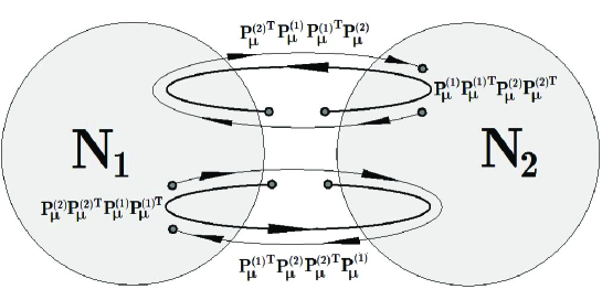
Figure 4: Self-adjoint operators for two interacting networks sharing the same set of nodes.

Any solution $\{\varphi^{(\alpha)},\psi^{(\alpha)}\}$ of the system (71), up to the possible partial isometries,

$${\bf G}^{(\alpha)}\varphi^{(\alpha)}=\psi^{(\alpha)},$$ (72)

also satisfies the system

$$\begin{array}[]{lcl}{\bf P}^{(2)}_{\mu}{}^{\top}{\bf P}^{(1)}_{\mu}{\bf P}^{(1)}_{\mu}{}^{\top}{\bf P}^{(2)}_{\mu}\psi^{(2)}&=&\left(\Lambda^{(1)}\Lambda^{(2)}\right)^{2}\psi^{(2)},\\ {\bf P}^{(1)}_{\mu}{}^{\top}{\bf P}^{(2)}_{\mu}{\bf P}^{(2)}_{\mu}{}^{\top}{\bf P}^{(1)}_{\mu}\psi^{(1)}&=&\left(\Lambda^{(1)}\Lambda^{(2)}\right)^{2}\psi^{(1)},\\ {\bf P}^{(1)}_{\mu}{\bf P}^{(1)}_{\mu}{}^{\top}{\bf P}^{(2)}_{\mu}{\bf P}^{(2)}_{\mu}{}^{\top}\varphi^{(1)}&=&\left(\Lambda^{(1)}\Lambda^{(2)}\right)^{2}\varphi^{(1)},\\ {\bf P}^{(2)}_{\mu}{\bf P}^{(2)}_{\mu}{}^{\top}{\bf P}^{(1)}_{\mu}{\bf P}^{(1)}_{\mu}{}^{\top}\varphi^{(2)}&=&\left(\Lambda^{(1)}\Lambda^{(2)}\right)^{2}\varphi^{(2)},\\ \end{array}$$ (73)

in which $\left(\Lambda^{(1)}\Lambda^{(2)}\right)^{2}\in[0,1].$ Operators in the l.h.s of the system (73) describe correlations between flows of random walkers which go through vertices following the links of either networks. They are represented by the non-negative symmetric matrices with orthonormal eigenvectors which can be subjected to the standard methods of the PCA analysis. Their spectrum can also be investigated by the methods discussed in the previous subsection.

It is convenient to represent the self-adjoint operators from the l.h.s. of (73) by the closed directed paths shown in the diagram in Fig. 4. Being in the self-adjoint products of transition operators, $P_{\mu}^{(\alpha)}$ corresponds to the flows of random walkers which depart from either networks, and $P_{\mu}^{(\alpha)}{}^{\top}$ is for those which arrive at the network $\alpha$. From Fig. 4 , it is clear that the self-adjoint operators in (73) represent all possible closed trajectories visiting both networks $\mathbf{N}_{1}$ and ${\bf N}_{2}$.

In general, given a complex system consisting of $n>1$ interacting networks operating on the same set of nodes, we can define $2^{n}$ self-adjoint operators related to the different modes of random walks. Then the set of network nodes can be separated into a number of essentially correlated segments with respect to each of self-adjoint operators.

5 Discussion and Conclusion

In the present paper, we have developed a self-consistent approach to complex transport networks based on the use of Markov chains defined on their graph representations.

From Euler’s time, urban design and townscape studies were the sources of inspiration for the network analysis and graph theory. It is common now that networks are the reality of urban renewals [41]. Flows of pedestrians and vehicles through a city are dependent on one another and that requests for organizing them in a network setting.

The networking is structurally contagious. In order to be able to master a network effectively, an authority should also constitute a network structure, probably as complicated as the one that it supervises. The governance and maintenance units supporting urban network renewals, negotiating performance targets, taking decisions, financing and eventually implementing them also form networks. A complex network of city itineraries that we can experience in everyday life appears as the result of multiple complex interactions between a number of transport, social, and economical networks.

It is intuitively clear that a complex network in equilibrium emerges from synergy and interplay between the topological structure shaped by a connected graph $G$ with some positive measures (masses) appointed for the vertices and some positive weights assigned to the edges, the dynamics described by the set of operators defined on $G$, and the properties of the embedding physical space specified by the metric length distances of the edges.

The approach we have discussed in the present paper helps to define an equilibrium state for complex transport networks and investigate its properties.

6 Acknowledgment

The work has been supported by the Volkswagen Foundation (Germany) in the framework of the project: ”Network formation rules, random set graphs and generalized epidemic processes” (Contract no Az.: I/82 418). The authors acknowledge the multiple fruitful discussions with the participants of the workshop Madeira Math Encounters XXXIII, August 2007, CCM - CENTRO DE CIÊNCIAS MATEMÁTICAS, Funchal, Madeira (Portugal).

References

- [1] D. Braess, ”Über ein Paradoxon aus der Verkehrsplannung”. Unternehmensforschung 12, 258-268 (1968).
- [2] G. Kolata, ”What if they closed the Street and nobody noticed?”, The New York Times, Dec. 25 (1990).
- [3] A. Manning, Ann. of Math. 110, 567-573 (1979).
- [4] M. Bourdon, L’Einseign. Math., 41 (2), 63-102 (1995) (in French).
- [5] T. Roblin, Ann. Inst. Fourier (Grenoble) 52, 145-151 (2002) (in French).
- [6] S. Lim, Minimal Volume Entropy on Graphs. Preprint arXiv:math.GR/050621, (2005).
- [7] J.G. Wardrop, Proc. of the Institution of Civil Engineers 1 (2), pp. 325-362 (1952).
- [8] M.J. Beckmann, C.B. McGuire, C.B. Winsten, Studies in the Economics of Transportation. Yale University Press, New Haven, Connecticut (1956).
- [9] B. Kuipers, Environment and Behavior 14 (2), pp. 202-220 (1982).
- [10] B. Hillier, J. Hanson, The Social Logic of Space. Cambridge University Press. ISBN 0-521-36784-0 (1984).
- [11] B. Hillier, Space is the Machine: A Configurational Theory of Architecture. Cambridge University Press. ISBN 0-521-64528-X (1999).
- [12] A. Penn, Space Syntax and Spatial Cognition. Or, why the axial line? In: Peponis, J. and Wineman, J. and Bafna, S., (eds). Proc. of the Space Syntax International Symposium, Georgia Institute of Technology, Atlanta, May 7-11 2001.
- [13] A. Smola and R. I. Kondor. ”Kernels and regularization on graphs”. In Learning Theory and Kernel Machines, Springer (2003).
- [14] D.J. Aldous, J.A. Fill, Reversible Markov Chains and Random Walks on Graphs. A book in preparation, available at www.stat.berkeley.edu/aldous/book.html.
- [15] L. Lovász, Bolyai Society Mathematical Studies 2: Combinatorics, Paul Erdös is Eighty, Keszthely (Hungary), p. 1-46 (1993).
- [16] F. Chung, Lecture notes on spectral graph theory, AMS Publications Providence (1997).
- [17] T. Morris, Computer Vision and Image Processing. Palgrave Macmillan. ISBN 0-333-99451-5 (2004).
- [18] K. Fukunaga, Introduction to Statistical Pattern Recognition, ISBN 0122698517, Elsevier (1990).
- [19] I.T. Jolliffe, Principal Component Analysis (2-nd edition) Springer Series in Statistics (2002).
- [20] J. Cohen, P. Cohen, S.G. West, L.S. Aiken, Applied multiple regression/correlation analysis for the behavioral sciences. (3rd ed.) Hillsdale, NJ: Lawrence Erlbaum Associates (2003).
- [21] B. Nadler, S. Lafon, R.R. Coifman and I.G. Kevrekidis, ”Diffusion maps, spectral clustering and reaction coordinate of dynamical systems”, Applied and Computational Harmonic Analysis: Special issue on Diffusion Maps and Wavelets, Vol. 21,113-127 (2006).
- [22] R. I. Kondor and J. Lafferty, ”Diffusion kernels on graphs and other discrete structures”. In C. Sammut and A. G. Hoffmann, editors, Machine Learning, Proceedings of the 19th International Conference (ICML 2002), pages 315-322. San Francisco, Morgan Kaufmann, (2002).
- [23] X. Zhu, Z. Ghahramani, J. Lafferty, ”Semi-supervised learning using gaussian fields and harmonic functions”. In Proc. 20th International Conf. Machine Learning, vol. 20, 912 (2003).
- [24] S. Saitoh, Theory of Reproducing Kernels and its Applications, Longman Scientific and Technical, Harlow, UK (1988).
- [25] G. Wahba, Spline Models for Observational Data, Vol. 59 of CBMS-NSF Regional Conference Series in Applied Mathematics, SIAM, Philadelphia (1990).
- [26] Shang-Keng Ma, Statistical mechanics, World Scientific (1985).
- [27] D. Volchenkov, Ph. Blanchard, Physical Review E 75(2), id 026104 (2007).
- [28] R. Albert, A.L. Barabási, Rev. Mod. Phys. 74, 47 (2002).
- [29] G. Bianconi, N. Gulbahce, A.E. Motter, Local structure of directed networks, E-print arXiv:0707.4084 [cond-mat.dis-nn] (27 July 2007).
- [30] D.J. Watts, S.H. Strogatz, Nature 393(6684), 440-442 (1998).
- [31] F. Chung, Annals of Combinatorics 9, 1-19 (2005).
- [32] L. Lovász, P. Winkler, Mixing of Random Walks and Other Diffusions on a Graph. Surveys in combinatorics, Stirling, pp. 119 154 (1995); London Math. Soc. Lecture Note Ser., vol. 218, Cambridge Univ. Press.
- [33] A. Bjöner, L. Lovász, P. Shor, Europ. J. Comb. 12, 283-291 (1991).
- [34] A. Bjöner, L. Lovász, J. Algebraic Comb. 1, 305-328 (1992).
- [35] S. Butler, Electronic Journal of Linear Algebra, 16 90 (2007).
- [36] N. Aubry, R. Guyonnet, R. Lima, J. Stat. Phys. 64, 683-739 (1991).
- [37] N. Aubry, Theor. and Comp. Fluid Dyn. 2, 339-352 (1991).
- [38] K. Karhunen, Ann. Acad. Sci. Fennicae A:1 (1944).
- [39] M. Loève, Probability Theory, van Nostrand, New York (1955).
- [40] N. Aubry, L. Lima, Spatio-temporal symmetries, Preprint CPT-93/P.2923, Centre de Physique Theorique, Luminy, Marseille, France (1993).
- [41] M. Haffner, M. Elsinga, Urban renewal performance in complex networks Case studies in Amsterdam North and Rotterdam South, W16 Institutional and Organizational Change in Social Housing Organization in Europe, Int. Conference on Sustainable Urban Areas, Rotterdam (2007).