Luminous Red Galaxies in hierarchical cosmologies

Abstract

Luminous red galaxies (LRGs) are much rarer and more massive than $L_{*}$ galaxies. Coupled with their extreme colours, LRGs therefore provide a demanding testing ground for the physics of massive galaxy formation. We present the first self-consistent predictions for the abundance and properties of LRGs in hierarchical structure formation models. We test two published models which use quite different mechanisms to suppress the formation of massive galaxies: the Bower et al. (2006) model, which invokes “AGN-feedback” to prevent gas from cooling in massive haloes, and the Baugh et al. (2005) model which relies upon a “superwind” to eject gas before it is turned into stars. Without adjusting any parameters, the Bower et al. model gives an excellent match to the observed luminosity function of LRGs in the Sloan Digital Sky Survey (with a median redshift of $z=0.24$) and to their clustering; the Baugh et al. model is less successful in these respects. Both models fail to match the observed abundance of LRGs at $z=0.5$ to better than a factor of $\approx 2$. In the models, LRGs are typically bulge dominated systems with stellar masses of $\approx 2\times 10^{11}h^{-1}M_{\odot}$ and velocity dispersions of $\sigma\sim 250{\rm kms}^{-1}$. Around half of the stellar mass in the model LRGs is already formed by $z\sim 2.2$ and is assembled into one main progenitor by $z\sim 1.5$; on average, only 25% of the mass of the main progenitor is added after $z\sim 1$. LRGs are predicted to be found in a wide range of halo masses, a conclusion which relies on properly taking into account the scatter in the formation histories of haloes. Remarkably, we find that the correlation function of LRGs is predicted to be a power law down to small pair separations, in excellent agreement with observational estimates. Neither the Bower et al. nor the Baugh et al. model is able to reproduce the observed radii of LRGs.

1 Introduction

Over the past few years, the most rapidly developing aspect of galaxy formation modelling has been the formation of massive galaxies (see Baugh 2006 for a review). On employing the standard White & Frenk (1991) model for the radiative cooling of gas in massive dark matter haloes, hierarchical models have tended to overproduce luminous galaxies. One pragmatic solution to this problem is to simply stop “by hand” the formation of stars from cooling flows in high circular velocity haloes (Kauffmann et al. 1993). A variety of physical mechanisms have been proposed to account for the suppression of the star formation rate in massive haloes, including: (i) the injection of energy into the hot gas halo to reduce its density and hence increase the cooling time (Bower et al. 2001; McCarthy et al. 2007); (ii) the fragmentation of the hot halo in a multi-phase cooling model (Maller & Bullock 2004); (iii) the complete ejection of gas from the halo in a “super wind” (Benson et al. 2003); (iv) the suppression of the cooling flow due to heating by an AGN (Croton et al. 2006; Bower et al. 2006); (v) thermal conduction of energy within the hot halo (Fabian et al. 2002; Benson et al. 2003). With such a range of possible physical processes to choose from, it is important to develop tests of the models which can distinguish between them. The mechanisms invoked to suppress the formation of bright galaxies could scale in different ways with redshift, leading to different predictions for the galaxy properties at intermediate and high redshift.

In this paper we present new tests of the physical processes invoked to suppress the formation of bright galaxies. At the present day, the bright end of the luminosity function is dominated by early-type galaxies with passively evolving stellar populations (e.g. Norberg et al. 2002). Here we focus on a subset of bright galaxies, luminous red galaxies (LRGs) and test the model predictions for the abundance and properties of these red, massive galaxies. LRGs were originally selected from the Sloan Digital Sky Survey (SDSS, York et al. 2000) on the basis of their colours and luminosities (Eisenstein et al. 2001). The red colour selection isolates galaxies with a strong 4000 Å   break and a passively evolving stellar population. The galaxies selected tend to be significantly brighter than $L_{*}$. The SDSS sample has a median redshift of $z\sim 0.3$. Recently, the construction of LRG samples has been extended to higher redshifts, using SDSS photometry and the 2dF and AAOmega spectrographs ($z\sim 0.5$, Canon et al. 2006; $z\sim 0.7$, Ross et al. 2007b). On matching the colour selection between the SDSS and 2SLAQ surveys, the evolution in the luminosity function of LRGs between $z\sim 0.3$ and $z\sim 0.5$ is consistent with that expected for a passively evolving stellar population (Wake et al. 2006). This has implications for the stellar mass assembly of the LRGs, with the bulk of the stellar mass appearing to have been in place a significant period before the LRGs are observed (Wake et al. 2006; Roseboom et al. 2006; Brown et al. 2007). Due to their strong clustering amplitude and low space density, LRGs are efficient probes of the large-scale structure of the Universe. The clustering of LRGs has been exploited to constrain cosmological parameters (e.g. Eisenstein et al. 2005; Hütsi 2006; Padmanabhan et al. 2007). The clustering of LRGs on smaller scales has been used to constrain the mass of the dark matter haloes which host these galaxies and to probe their merger history (Zehavi et al. 2005; Masjedi et al. 2006; Ross et al. 2007a).

To date, surprisingly little theoretical work has been carried out to see if LRGs can be accommodated in hierarchical cosmologies, and only very simple models have been used. Granato et al. (2004) considered a model for the formation of spheroids in which the quasar phase of AGN activity suppresses star formation in massive galaxies, and found reasonable agreement with the observed counts of red galaxies at high redshift. Hopkins et al. (2006) used the observed luminosity function of quasars along with a model for the lifetime of the quasar phase suggested by their numerical simulations to infer the formation history of spheroids, and hence red galaxies. Conroy, Ho & White (2007) use N-body simulations to study the merger histories of the dark matter haloes that they assume host LRGs. Using a simple model to assign galaxies to progenitor haloes, they argue that mergers of LRGs must be very efficient, or that LRGs are tidally disrupted, in order to avoid populating cluster-sized haloes with too many LRGs. Barber et al. (2007) used population synthesis models coupled with assumptions about the star formation histories of LRGs to infer the age and metallicity of their stellar populations.

Here we present the first fully consistent predictions for LRGs from hierarchical galaxy formation models, using two published models, namely Baugh et al. (2005) and Bower et al. (2006). These models, both based on the GALFORM semi-analytical code (Cole et al. 2000), carry out an ab initio calculation of the fate of baryons in a cold dark matter universe. The models predict the star formation and merger histories for the whole of the galaxy population, producing broad-band magnitudes in any specified pass band. Hence, LRGs can be selected from the model output using the same colour and luminosity criteria that are applied to the real observational data. The models naturally predict which dark matter haloes host LRGs. As we will see later, a key element in shaping the “halo occupation distribution” of LRGs is the scatter in the merger histories of dark matter haloes, which has been ignored in previous analyses.

This paper extends the work of Almeida et al. (2007) in which we tested the predictions of the same two galaxy formation models for the scaling relations of spheroids, such as the radius-luminosity relation and the fundamental plane. The galaxies we consider in this paper represent a much more extreme population than those studied in our previous work. LRGs are much rarer and significantly brighter than $L_{*}$ galaxies and even than the early-type population as a whole. In this paper we concentrate on massive red galaxies at low and intermediate redshifts where large observational samples exist; in a companion study, we test the model predictions for “extremely red objects” at high redshift (González-Pérez et al., in preparation). We remind the reader of the key features of the two models in Section 2 (see also the comparison given in Almeida et al. 2007). In Section 3, we explain the selection of LRGs and show some basic predictions for the abundance and properties of LRGs. In Section 4, we present predictions for the clustering of LRGs and in Section 5 we examine how the stellar mass of LRGs is built up in the models. Our conclusions are given in Section 6.

2 Modelling the galaxy population

In this section, we give a brief outline of the two versions of the GALFORM model which we study in this paper, the Baugh et al. (2005) and the Bower et al. (2006) models. An introduction to the semi-analytical approach to modelling the formation of galaxies can be found in the review by Baugh (2006). The GALFORM model itself is described in detail by Cole et al. (2000). The superwind feedback model used by Baugh et al. was introduced by Benson et al. (2003) and is also discussed by Nagashima et al. (2005a).

Both the Baugh et al. and Bower et al. models are calibrated against a subset of the observational data available for local galaxies. The Bower et al. model gives a somewhat better match to the sharpness of the break in the optical and near-infrared galaxy luminosity functions than the Baugh et al. model. Other outputs from the models besides these local calibrating data are model predictions. The Bower et al. model also gives an excellent match to the evolution of the stellar mass function inferred from observations. The Baugh et al. model has been tested extensively and reproduces a wide range of datasets: the number counts and redshift distribution of galaxies in the sub-mm and the luminosity function of Lyman-break galaxies (Baugh et al. 2005), the mid-infrared luminosity functions as measured using Spitzer (Lacey et al. 2008), the metal content of the intracluster medium (Nagashima et al. 2005a), the metallicity of elliptical galaxies (Nagashima et al. 2005b), the abundance of Lyman-alpha emitters and their properties (Le Delliou et al. 2005; 2006) and some of the scaling relations of elliptical galaxies, including the fundamental plane (Almeida et al. 2007).

We emphasize that in this paper we do not vary any of the parameters which specify the Baugh et al. and Bower et al. models. Our goal is to expand the tests of the published models to include the predictions for the abundance and properties of luminous red galaxies. None of the datasets originally used to set the model parameters had any explicit connection to bright red galaxies at the redshifts of interest in this paper. The results we present are therefore genuine predictions of the model and represent a powerful, “blind” test of the semi-analytical methodology. A key constraint in setting the model parameters is the requirement that they reproduce as closely as possible the bright end of the present day galaxy luminosity function, which is dominated by galaxies with red colours and passive stellar populations (e.g. Norberg et al. 2002). Matching the observed properties of LRGs therefore acts as a test of the evolution of the bright end of the luminosity function in the models, as traced by galaxies with passive stellar populations.

A full description of the two models is, of course, given in the original papers. A comparison of the ingredients in the models can be found in Almeida et al. (2007; see also Lacey et al. 2008). Here, for completeness, we give a brief summary of where the principal differences lie between the models:

• Dark matter halo merger trees. The Baugh et al. model employs halo merger trees generated using the Monte Carlo algorithm introduced by Cole et al. (2000). In the Bower et al. model, the halo merger histories are extracted from the Millennium Simulation (Springel et al., 2005). A comparison of the predictions of galaxy formation models made using these two approaches to produce merger trees shows that they yield similar results for galaxies brighter than a threshold magnitude which is set by the mass resolution of the N-body trees (Helly et al., 2003). In the case of the Millennium merger trees, this limit is several magnitudes fainter than $L_{*}$ and so has no impact on the results presented in this paper, which concern much brighter galaxies.

• Feedback processes. Both models use the “standard” supernova driven feedback common to essentially all semi-analytical models (though with different values for the parameters). In this scenario, supernovae and stellar winds reheat cooled gas and thus regulate the supply of gas available for subsequent star formation. The models differ in how they treat the reheated gas. In the Baugh et al. model, the reheated gas is not considered as being available to cool again from the hot halo until the mass of the halo has doubled. At this point, the gas heated by supernova feedback is added to the hot gas halo of the new dark matter halo. Bower et al., on the other hand, incorporate the reheated gas into the hot halo after a delay which is a multiple of the dynamical time of the dark matter halo.

  The two models use different feedback mechanisms to counter the overproduction of bright galaxies, which was a long-standing problem for hierarchical models (see Baugh 2006). Baugh et al. invoke a wind which ejects cold gas from galaxies at a rate which is a multiple of the star formation rate (see Benson et al., 2003). The gas thus ejected is not allowed to recool, even in more massive haloes. This is another “channel” for the energy released by supernovae to couple to the cold gas reservoir available for star formation which operates alongside the feedback mechanism described in the previous paragraph. The superwind and the “standard” supernova feedback have distinct parameterizations in terms of the star formation rate, and differ in the fate of the reheated gas, as discussed above (see Lacey et al. 2008 for an expanded discussion and for the respective equations). There is observational evidence for superwind outflows in the spectra of Lyman-break galaxies and in local starburst galaxies (Adelberger et al., 2003; Wilman et al., 2005). In the Bower et al. model, the cooling of gas is suppressed in massive haloes due to the heating of the halo gas by the energy released by the accretion of matter onto a central supermassive black hole. The growth of the black hole is based on the model described by Malbon et al. (2007).

• Hot gas distribution Both models adopt a density profile for the hot gas halo of the form $\rho\propto(r^{2}+r^{2}_{\rm core})^{-1}$. In the Bower et al. model, $r_{\rm core}$ is kept fixed at 0.1 of the virial radius. In the case of Baugh et al., the core radius is initial set to be one third of the scale length of the dark matter density profile (Navarro, Frenk & White 1997). The core radius evolves with time in this model, as it is recomputed when a new halo forms to take into account that the densest, lowest entropy gas has cooled preferentially from the central regions of the progenitor haloes (see Cole et al. 2000).

• Star formation. In both models, there are two modes of star formation, quiescent star formation, which occurs in galactic disks, and starbursts. Baugh et al. adopt a quiescent star formation timescale which is independent of the dynamical time of the galaxy, unlike Bower et al.. Hence, galactic disks tend to be gas rich at high redshift in the Baugh et al. model, whereas they are gas poor in the Bower et al. model; this means that starbursts triggered by galaxy mergers tend to be more intense in the Baugh et al. model than in Bower et al. The later model also allow bursts which are the result of a galactic disk becoming dynamically unstable.

• Stellar Initial Mass Function (IMF). Both models adopt a standard solar neighbourhood IMF, the Kennicutt (1998) IMF, for quiescent star formation. Bower et al. also use this IMF in starbursts, whereas Baugh et al. invoke a top heavy IMF, which is the primary ingredient responsible for this model’s successful reproduction of the number counts of sub-mm galaxies. The yield we adopt is consistent with the choice of IMF. The choice of a top-heavy IMF in starbursts is controversial, but has been tested successfully against the metal content of the intra-cluster medium (Nagashima et al. 2005a) and the metallicity of elliptical galaxies (Nagashima et al. 2005b).

• Cosmology. Baugh et al. use the canonical ($\Lambda$CDM) parameters: matter density, $\Omega_{0}=0.3$, cosmological constant, $\Lambda_{0}=0.7$, baryon density, $\Omega_{b}=0.04$, a normalization of density fluctuations given by $\sigma_{8}=0.93$ and a Hubble constant $h=0.7$ in units of 100 km s^-1 Mpc^-1. (Note in Baugh et al., the value of $\sigma_{8}$ is reported as 0.9, when this should be $\sigma_{8}=0.93$.) Bower et al. adopt the cosmological parameters of the Millennium simulation (Springel et al. 2005), which are in better agreement with the latest constraints from measurement of the cosmic microwave background radiation and large scale galaxy clustering (e.g. Sanchez et al. 2006): $\Omega_{0}=0.25$, $\Lambda_{0}=0.75$, $\Omega_{b}=0.045$, $\sigma_{8}=0.9$ and $h=0.73$.

3 LRG selection and basic properties

In this section, we present the predictions of the Baugh et al. and Bower et al. models for the basic properties of low and intermediate redshift luminous red galaxies (LRGs) and compare these with observational results from the SDSS and 2SLAQ LRG samples. LRGs are a subset of the overall early-type population with extreme luminosities and colours, so it is essential to match their selection criteria as closely as possible in order to make a meaningful test of the model predictions. We begin by reviewing the colour and magnitude selection used in these surveys (§3.1), before moving on to examine the predictions for the abundance of LRGs (§3.2). This issue is dealt with in further detail in §4, in which we focus on the clustering of LRGs. In §3.3, we compare the model predictions for a range of LRG properties with observations. Finally, in §3.4, we discuss the physical reasons for the differences between the predictions of the two models.

3.1 Sample selection: SDSS and 2SLAQ LRGs

The basic aim of LRG surveys is to select intrinsically bright galaxies which have colours consistent with those expected for a passively evolving stellar population (Eisenstein et al., 2001). The selection criteria used in the SDSS LRG and 2dF-SDSS LRG and QSO (2SLAQ) surveys are targetted at different redshift intervals and pick up very different number densities of objects. Full descriptions of the design of the respective surveys can be found in Eisenstein et al. (2001) and Cannon et al. (2006).

Below, for completeness, we give a summary of the colour and magnitude ranges which define the LRG samples. In the case of the observational samples, Petrosian magnitudes were used for apparent magnitude selection and SDSS model magnitudes were used for colour selection. The SDSS filter system is described in Fukugita et al (1996). In the case of GALFORM galaxies, we use the total magnitude. We consider two output redshifts in the GALFORM models, chosen to be close to the median redshifts of the observational samples; $z=0.24$ to compare with SDSS LRGs and $z=0.50$ to match the 2SLAQ LRGs.

In the case of the SDSS, two combinations of the $g-r$ and $r-i$ colours are formed:

$$c_{\perp} = (r-i)-(g-r)/4-0.177$$ (1)

$$c_{\parallel} = 0.7(g-r)+1.2[(r-i)-0.177].$$ (2)

The following conditions are then applied to select LRGs:

$$r_{\rm petro} < 19.2$$ (3)

$$r_{\rm petro} < 13.116+c_{\parallel}/0.3$$ (4)

$$|c_{\perp}| < 0.2$$ (5)

In the case of 2SLAQ, somewhat different colour combinations are used:

$$d_{\perp} = (r-i)-(g-r)/8$$ (6)

$$d_{\parallel} = 0.7(g-r)+1.2[(r-i)-0.177].$$ (7)

The selection criteria applied in the case of 2SLAQ are:

$$17.5 < i\,<\,19.8$$ (8)

$$0.5 < g-r\,<\,3$$ (9)

$$r-i < 2$$ (10)

$$d_{\perp} > 0.65$$ (11)

$$d_{\parallel} > 1.6$$ (12)

The colour equations (Eqs. 1, 2 6, 7) and the conditions applied to them (Eqs. 5, 11, 12) are designed to locate galaxies with appreciable 4000 Å breaks in the $(g-r)$ vs $(r-i)$ plane over the redshift intervals of the two surveys (see Eisenstein et al 2001 and Cannon et al. 2006 for further details).

As we have already commented, these two sets of selection criteria give quite different number densities of LRGs. Here we do not attempt to tune the selection to match objects in the 2SLAQ LRG sample with those from the SDSS LRG sample. This was done by Wake et al. (2008), whose motivation was to study the evolution of the LRG luminosity function. Our aim instead is to test the galaxy formation models, so trying to match the selection to pick out similar objects between the two redshifts is not necessary.

3.2 Luminosity Function

The luminosity function is the most basic description of any galaxy population and is arguably the key hurdle for a model of galaxy formation to negotiate before considering other predictions. It is important to bear in mind that LRGs represent only a small fraction of the galaxy population as a whole, as can be seen by comparing the integrated space densities quoted in Table 1 with the abundance of $L_{*}$ galaxies, which is around an order of magnitude higher. Reproducing the abundance of such rare galaxies therefore represents a strong challenge for any theoretical model.

Figure 1: The luminosity function of luminous red galaxies plotted as a function of apparent magnitude. The upper panel shows the SDSS LRG luminosity function at $z=0.24$, the median redshift of this sample, and the lower panel shows the results for the 2SLAQ sample at its median redshift, $z=0.5$. The upper axis labels show the absolute magnitude for reference (calculated from the apparent magnitude by subtracting the appropriate distance modulus for each panel). In each panel, the dashed line shows the number density of LRGs predicted by the Baugh et al. model and the dotted line shows the prediction of the Bower et al. model. The observational estimates are shown by the stars. The error bars on the model predictions show the Poisson error due to the finite number of galaxies simulated.

In Fig. 1, we compare the predictions of the GALFORM models for the luminosity function of LRGs with observational estimates. This determination of the observed 2SLAQ and SDSS luminosity functions is different from that presented in Wake et al. (2006). Here, we have estimated the observed luminosity functions in such a way as to minimize the corrections necessary to compare to the models. We have restricted both samples to tight redshift ranges around the model output redshifts, $0.22<z<0.26$ for the case of SDSS and $0.48<z<0.54$ for 2SLAQ. We then use simple K+e corrections derived from Bruzual & Charlot (2003) stellar population synthesis models (see Wake et al. 2006) to correct the SDSS LRG magnitudes to z = 0.24 and the 2SLAQ LRG magnitudes to z = 0.5. Since the redshift ranges considered here are so close to the target redshift, these corrections are very small, $<0.01$ mags. The SDSS catalogue is then cut at $i^{0.24}<17.5$ and the 2SLAQ catalogue is cut at $i^{0.5}<19.6$. Both of these cuts are brighter than the magnitude limits of each survey and within the limited redshift ranges effectively produce volume-limited samples. The final samples contain 5217 and 2576 LRGs within 8.5x10${}^{7}{\rm Mpc}^{3}$ and 3.9x10${}^{7}{\rm Mpc}^{3}$ for SDSS and 2SLAQ respectively (assuming $h=0.7=H_{0}/(100{\rm kms}^{-1}{\rm Mpc}^{-1}$). Since the samples are approximately volume-limited it is trivial to produce the luminosity function including a correction for incompleteness in each survey (see Wake et al. 2006). The integrated number densities of LRGs in the two surveys are listed in Table 1 after applying the respective completeness corrections.

In view of the fact that no model parameters have been adjusted in order to “tune” the predictions to better match observations of LRGs, both models come surprisingly close to matching the number density of LRGs in the SDSS sample, as Table 1 shows. In fact, the Baugh et al. model slightly overpredicts the space density of LRGs at $z=0.24$ by 13%, whereas the Bower et al. model underpredicts only by 10%. However, Fig. 1 shows that the Baugh et al. actually gives a poor match to the shape of the luminosity function, predicting too many bright LRGs. Although the difference looks dramatic on a logarithmic scale, the discrepancy has little impact on the integrated space density.

At the median redshift of the 2SLAQ sample, the comparison with the observational estimate of the luminosity function of LRGs is less impressive. The Baugh et al. model now underpredicts the abundance of LRGs by a factor of $2$. Alternatively, the discrepancy is equivalent to a shift of about one magnitude in the $i$-band. The Bower et al. model fares analogously, predicting around $100\%$ more LRGs than are seen in the 2SLAQ sample. This suggests that neither model is able to accurately follow the evolution of the luminosity function of very red galaxies over such a large lookback time (when the age of the universe is only around 60% of its present day value). The abundance of LRGs is therefore quite sensitive to the way in which feedback processes are implemented in massive haloes.

Sample	SDSS	2SLAQ
	($z=0.24$)	($z=0.50$)
	($10^{-5}$ Mpc-3)	($10^{-5}$ Mpc-3)
Observed space density	3.30	8.56
Baugh et al. prediction	3.74	4.75
Bower et al. prediction	2.99	18.11

Table 1: The space density of LRGs in the SDSS and 2SLAQ samples estimated at their median redshifts, compared with the predictions of the Baugh et al. and Bower et al. models. The number density in the table are quoted in units of $10^{-5}$ Mpc^-3. (The relevant $h$ is used for each model; for the data, $h=0.7$ is assumed.)

3.3 Properties of LRGs

In this section, we present a range of predictions for the properties of galaxies which satisfy the LRG selection criteria defined in section 3.1, for both the Baugh et al. and Bower et al. models, comparing with observational results whenever possible. We remind the reader that the models do not reproduce exactly the shape and normalization of the observed luminosity function of LRGs as seen in S 3.2, but instead bracket the observed abundances. Rather than perturb the selection criteria applied the model galaxies to better match the observed abundances, we have retained the full LRG selection criteria (§3.1) so that the model galaxies have the same colours and magnitudes as observed LRGs.

3.3.1 Stellar mass

Figure 2: The predicted stellar masses of model luminous red galaxies at $z=0.24$ (upper panel) and $z=0.50$ (lower panel). The predictions of the Baugh et al. model are shown by the dashed histograms and those of the Bower et al. model by the dotted histograms. The distributions are normalized to give $\sum_{i}f_{i}=1$.

The predicted stellar masses of LRGs are plotted in Fig. 2. As expected from the high luminosities of LRGs, these galaxies exhibit large stellar masses. At $z=0.24$ the stellar masses range from $\sim 1\times 10^{11}$ to $5\times 10^{11}$ h^-1M_⊙, with a median of $1.7\times 10^{11}$ h^-1M_⊙. At $z=0.50$, the distribution shifts to lower stellar masses, with a median value of $\sim 1\times 10^{11}$ h^-1M_⊙. The scatter in the distribution of stellar masses predicted by the Baugh et al. model is somewhat larger than that in the Bower et al. model at $z=0.24$. The median stellar mass is a property for which the two models agree closely, indicating that stellar mass is a robust prediction which is fairly insensitive to the details of the implementation of the physics of galaxy formation. The difference in the selection criteria applied to the two samples is responsible for picking up objects of quite different stellar masses. We shall see in subsequent comparisons that this basic difference between the LRG samples is responsible for differences in other model predictions.

3.3.2 Morphological mix

Figure 3: The predicted bulge-to-total luminosity ratio in the rest-frame V-band for luminous red galaxies. The upper panel shows the predictions of the Baugh et al. (dashed histogram) and Bower et al. models (dotted histogram) at $z=0.24$. The lower panel displays the distributions predicted for LRGs at $z=0.50$. The distributions are normalized to give $\sum_{i}f_{i}=1$.

Redshift	Baugh et al.	Bower et al.
	[0,0.4]:[0.4,0.6]:[0.6,1.0]	[0,0.4]:[0.4,0.6]:[0.6,1.0]
$z=0.24$	12:2:86	21:17:62
$z=0.50$	21:6:73	24:22:54

Table 2: The predicted morphological mix of luminous red galaxies, at $z=0.24$ and $z=0.50$, for the Baugh et al. and Bower et al. models. The three values quoted for each model show the percentage of galaxies with bulge-to-total luminosity ratios of $B/T<0.4$, $0.4\leq B/T\leq 0.6$ and $B/T>0.6$.

Figure 4: The rest-frame V-band luminosity-weighted age of the stellar populations of LRGs at $z=0.24$ (upper panel) and $z=0.5$ (lower panel). As before, the predictions of the Baugh et al. model are shown by the dashed histograms and those of the Bower et al. model by the dotted histograms. The histograms are normalized as in Fig. 2.

Figure 5: The predicted distribution of the rest-frame V-band luminosity-weighted metallicity of LRGs. The upper panel displays the Baugh et al. (dashed histogram) and Bower et al. (dotted histogram) models at $z=0.24$ and the lower panel shows the predictions at $z=0.50$. The histograms are normalized as in Fig. 2.

The bulge-to-total luminosity ratio, B/T, is often used as an indicator of the morphological type of a galaxy in semi-analytical models (see e.g. Baugh, Cole & Frenk 1996). The B/T ratio is correlated with Hubble T-type, a subjective classification parameter relying upon the identification of features such as spiral arms and galactic bars, though there is considerable scatter around this relation (Simien & de Vaucouleurs 1986). In the B-band, galaxies with $B/T<0.4$ correspond approximately to the T-types of late-type or spiral galaxies, those with $B/T>0.6$ overlap most with elliptical galaxies and the intermediate values, $0.4<B.T<0.6$ correspond to lenticulars. In Fig. 3 we plot the predicted distribution of the bulge-to-total ratio in the rest-frame V-band, B/T_V, for the Baugh et al. and Bower et al. models, at $z=0.24$ (upper panel) and $z=0.50$ (lower panel). The results are also summarized in Table 2, where the fraction of galaxies in intervals of B/T_V ratio are calculated.

In both models, the SDSS and 2SLAQ LRG samples are predicted to be mainly composed of bulge-dominated galaxies, which account for more than $\sim 60\%$ of the LRG population. However, the models suggest that the LRG samples contain an appreciable fraction ($\sim 20\%$) of late-type, disk-dominated systems. These galaxies meet the LRG colour selection criteria primarily because they have old stellar populations. Another prediction is that the fraction of bulge dominated galaxies is higher in the SDSS sample than in the 2SLAQ sample.

The distributions of $B/T$ ratios predicted by the two models show substantial differences, particularly in the intermediate ratio range, which corresponds roughly to S0 types. This difference is not due to any single model ingredient, but is more likey to be the result of the interplay between several phenomena. As outlined in Section 2 (see also Almeida et al. 2007), both models invoke galaxy mergers as a mechanism for making spheroids, either by the rearrangement of stellar disks or through triggering additional star formation. Bower et al. also consider starbursts resulting from disks being dynamically unstable to bar formation. In the Baugh et al. model, around 30% of the total star formation takes place in merger driven starbursts. This figure is much lower in the Bower et al. case, because galactic disks tend to be gas poor at high redshift in this model, as explained in Section 2. In the Bower et al. model, starbursts resulting from the collapse of unstable disks dominate bursts driven by galaxy mergers. Baugh et al. allow minor mergers to trigger starbursts, if the primary disk is gas rich. We have tested that removing these starbursts does not have a major impact on the distribution of $B/T$ values.

3.3.3 Stellar populations

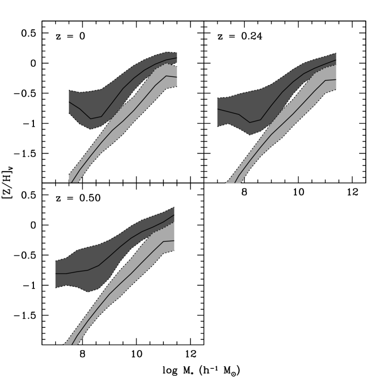
Figure 6: The rest-frame V-band luminosity weighted metallicity – stellar mass relation for ellipticals (i.e. galaxies with a bulge-to-total stellar mass ratio greater than 0.6). The light and dark gray shaded regions show the distributions for the Bower et al. and the Baugh et al. models, respectively. Each panel corresponds to a different redshift, as indicated by the key. The solid line shows the median metallicity for stellar mass bins. The shaded regions are enclosed by the 10 and 90 percentiles of the distribution.

The luminosity-weighted age of a stellar population is a measure of the age of the stars in a galaxy. The predicted distributions of the rest-frame V-band luminosity-weighted age of LRGs are plotted in Fig. 4. This plot reveals that LRGs have stellar populations with luminosity-weighted ages ranging from 4 to 8 Gyr in the Bower model, and from 2 to 6 Gyr in the Baugh et al. model, at $z=0.24$ (i.e. when the Universe was $\sim 80\%$ of its current age). At $z=0.50$ ($60\%$ of the current age of the Universe), galaxies in the Bower et al. model show, again, older stellar ages than those in the Baugh et al. model: the median of the distribution for LRGs in the Bower et al. model is $\approx 4.2$ Gyr, whereas for the Baugh et al. model it is $3.2$ Gyr. The difference in the age of the Universe between these redshifts is around $2$ Gyr (the value is slightly different for each model due to the different choice of the values of the cosmological parameters), and therefore accounts for the bulk of the difference in the ages of the SDSS and 2SLAQ samples. The model LRGs are therefore composed predominantly of old stellar populations and resemble those of observed early-type galaxies (e.g. Trager et al., 2000; Gallazzi et al., 2006). Furthermore, our results are in excellent agreement with the analysis by Barber et al. (2007). Barber et al. used stellar population synthesis models to fit the spectra of 4391 LRGs from the SDSS, finding matches for ages in the range from 2 to 10 Gyrs, with a peak in the distribution around 6 Gyrs. The difference in the ages predicted by the Baugh et al. and Bower et al. models has its origins in the different implementations of gas cooling and feedback applied in massive dark matter haloes. De Lucia et al. (2006) show that the suppression of gas cooling due to AGN feedback tends to increase the age of the stellar population in the galaxies hosted by haloes with quasistatic hot gas atmospheres. Note that in hierarchical models, the age of the stars in a galaxy is not the same as the age of the galaxy: the age of the stellar population can greatly exceed the age of the galaxy, with stars forming in the galaxy’s progenitors, which are later assembled into the final galaxy through mergers (e.g. Baugh et al. 1996; Kauffmann 1996; De Lucia & Blaizot 2007). We revisit this point in Section 5.

Fig. 5 shows the predicted distribution of the V-band luminosity-weighted metallicity for LRGs. There is little change in the luminosity weighted-metallicity between the two LRG samples in the Baugh et al. model. In the Bower et al. model, there is a modest decrease in metallicity of almost +0.2dex between $z=0.24$ and $z=0.5$. To help in the interpretation of these predictions it is instructive to plot the metallicity–stellar mass relation for spheroids at different redshifts (N.B. here, we consider any galaxy with a bulge-to-total stellar mass ratio in excess of 0.6, not just LRGs; we note that the metallicity–stellar mass relation is similar for galaxies with bulge-to-total ratios below 0.6). We recall that the typical stellar mass of LRGs is predicted to change by a factor of two between the $z=0.5$ and $z=0.24$ samples, from $\log(M_{*}/h^{-1}M_{\odot})\sim 11$ to $\log(M_{*}/h^{-1}M_{\odot})\sim 11.3$. The predicted evolution of the stellar mass–metallicity relation for the Baugh et al. and Bower et al. models is shown in Fig. 6. There is little evolution in the locus of the metallicity–mass relation. Between $z=0.5$ and $z=0.24$, the metallicity–stellar mass relation in the Baugh et al. model flattens at the high mass end. Hence, the change in metallicity expected due to an increase in stellar mass by a factor of 2 using the metallicity–mass relation predicted at $z=0.5$ is largely cancelled out by the change in slope of the metallicity – mass relation at $z=0.24$. In the Bower et al. model, the metallicity–mass relation has a kink at $\log(M_{*}/h^{-1}M_{\odot})\sim 11$, and is flat for the most massive galaxies over the whole of the redshift range plotted in Fig. 6. The evolution seen in the Bower et al. model is therefore due to the presence at $z=0.5$ of LRGs with masses $<10^{11}h^{-1}M_{\odot}$ which come from the steep part of the metallicity–mass relation; at $z=0.24$, only LRGs from the flat part of the metallicity–mass relation are sampled due to the increase in stellar mass.

Fig. 5 shows that the Bower et al. model displays a different metallicity distribution from the Baugh et al. model, predicting luminosity-weighted metallicities lower by a factor of $\sim 2$. This difference is entirely due to the choice of IMF used in the models. We remind the reader that, in the Baugh et al. model, stars which form in merger driven bursts are assumed to be produced with a flat IMF, whereas in the Bower et al. model, a Kennicutt (1993) IMF is adopted in all modes of star formation. The yield adopted is consistent with the choice of IMF. For a flat IMF, the yield is over six time larger than the yield expected from a Kennicutt IMF. As noted by Nagashima et al. (2005b), the metal abundances for galaxies in the Baugh et al. model are higher by a factor of 2-3 than is the case for a model using a Kennicutt IMF. Intriguingly, Barber et al. (2007) also favour high metallicities in their simple fits to the spectra of SDSS LRGs, finding best fitting models in the range $-0.6\la[{\rm Z/H}]\la 0.4$, which they argue is evidence in favour of LRGs forming stars with a top-heavy IMF.

3.3.4 Are LRGs central or satellite galaxies?

Redshift	Baugh et al.	Bower et al.
$z=0.24$	0.25	0.32
$z=0.50$	0.21	0.30

Table 3: The predicted fraction of satellite galaxies in the luminous red galaxies samples at $z=0.24$ and $z=0.50$.

In the models, the most massive galaxy within a dark matter halo is referred to as the “central” galaxy and any other galaxies which also reside in the halo are referred to as “satellites” (see Baugh 2006). In the majority of semi-analytical models, this distinction is important because gas which cools from the hot gas halo is directed onto the central galaxy, and satellite galaxies can merge only with the central galaxy. The fraction of luminous red galaxies which are satellite galaxies in the models is given in Table 3; more than 25% of LRGs at $z=0.24$ are satellite galaxies with a slight decrease in this fraction for the 2SLAQ sample. The fraction of satellite galaxies has important consequences for the small scale clustering of LRGs, as we shall discuss in Section §4.

3.3.5 Radii

Figure 7: The predicted half mass radii of luminous red galaxies. The upper and lower panels display the predictions of the Baugh et al. (dashed histograms) and Bower et al. models (dotted histograms), at $z=0.24$ and $z=0.5$ respectively. The histograms are normalized as in Fig. 2. The arrow shows the median de Vaucouleur’s radius of the observed SDSS LRGs.

The distribution of the radii of model LRGs is shown in Fig. 7. We plot the half-mass radius of the model galaxies, taking the mass weighted average of the disk and bulge components. The calculation of the linear sizes of galaxies in GALFORM takes into account the conservation of the angular momentum of cooling gas and the conservation of energy of merging galaxies (Cole et al. 2000). This prescription was tested against observations of bulge dominated SDSS galaxies by Almeida et al. (2007). Overall, Almeida et al. found that the predicted sizes of spheroids in the Baugh et al. model matched the observed sizes reasonably well, except for galaxies much brighter than $L_{*}$. These bright galaxies are predicted to be a factor of up to three smaller than observed by Bernardi et al. (2005). In the Bower et al. model, the brightest spheroids are predicted to be even smaller than in the Baugh et al. model. The same trend is seen in the predictions for the sizes of LRGs shown in Fig. 7. At $z=0.24$, the median of the distribution of LRG half-light radii in the Baugh et al. model occurs at $\sim 1.76h^{-1}{\rm kpc}$. In the Bower et al. model, this peak is at a radius that is around a factor of 2 smaller. At $z=0.5$, the median of the two model distributions differ by a smaller factor, $\approx 1.8$, although there is little evolution in the distributions from $z=0.5$ to $z=0.24$. The observed radii of SDSS LRGs (as extracted from the online database) are larger than the model predictions, with a median de Vaucouleur’s radius of $6.6h^{-1}{\rm kpc}$. The observational estimate of the LRG radius is obtained by fitting a de Vaucouleur’s profile convolved with a seeing disk. In this case the seeing is restricted to be no worse than 1.4 arcseconds, which corresponds to a scale of $3.7h^{-1}{\rm kpc}$ at the median redshift of the SDSS sample. Thus the tail of small scale-length galaxies predicted by the models would not be observable. However, the observed distribution of LRG sizes has few galaxies close to the seeing limit, so this is does not affect the estimation of the median size of SDSS LRGs.

3.3.6 Velocity dispersion

Figure 8: The predicted one-dimensional velocity dispersion of luminous red galaxies in the Baugh et al. (dashed lines) and Bower et al. models (dotted lines). The upper panel shows the distributions at $z=0.24$ and the lower panel at $z=0.50$. The histograms are normalized as in Fig. 2. The median velocity dispersion of the observed SDSS LRGs is represented by the arrow.

Fig. 8 shows the distribution of the one-dimensional velocity dispersion of the bulge component of model LRGs, $\sigma_{\rm 1D}$. This is calculated from the effective circular velocity of the bulge, $V_{\rm c,bulge}$, using $\sigma_{\rm 1D}=(1.1/\sqrt{3})V_{\rm c,bulge}$, where $\sigma_{\rm 1D}$ is assumed to be isotropic. The circular velocity at the half mass radius of the bulge is a model output which is computed taking into account the angular momentum and mass of the disk and bulge, and the gravitational contribution of the baryons and dark matter (see Cole et al. 2000 for further details). The factor of $1.1$ is an empirical adjustment introduced by Cole et al. (1994) which we have retained to facilitate comparison with predictions for the more general population of spheroids presented in Almeida et al. (2007). At $z=0.24$, both models predict velocity dispersions in the range $220$–$400{\rm kms}^{-1}$, with a median around $320{\rm kms}^{-1}$. Between $z=0.24$ and $z=0.5$, the predicted distribution of LRG velocity dispersions shifts to lower values by $\Delta\log\sigma\approx 0.1$. The bulk of this evolution is due to the change in stellar mass between the LRG samples (see Fig. 16 of Almeida et al., 2007). The median velocity dispersion for SDSS LRGs is $\sigma=250{\rm kms}^{-1}$, which is somewhat smaller than the model predictions.

3.4 Why do the two models give different predictions?

In §3.2, we demonstrated that the predictions of the Bower et al. model for the luminosity function of LRGs are in better agreement with the observations than those of the Baugh et al. model. In particular, at $z=0.24$, the Bower et al. model gives a very good match both to the shape of the observed luminosity function and the integrated number density of LRGs, matching the observed density at the 10% level. The Baugh et al. model predicts too many LRGs at this redshift, particularly at the bright end.

We saw in Section 2 that there are several areas in which the input physics and parameter choices differ between the two models. Although our aim in this paper is to test published models and not to tweak the results to fit the LRG population, it is instructive to vary some of the parameters in the Baugh et al. model to see if the predictions for the number of LRGs improve. We varied several model ingredients (e.g. strength of superwind feedback, star formation timescale, burst duration, choice of IMF in bursts, criteria for triggering a starburst following a galaxy merger) and found that in all cases, the resulting change in the luminosity function of LRGs was driven by a change in the overall luminosity function, i.e. if the number of bright LRGs increased, the luminosity function of all galaxies was found to brighten by a similar amount. Since a model is only deemed successful if it reproduces as closely as possible the overall galaxy luminosity function, none of these variant models is acceptable without further parameter changes to reconcile the overall luminosity function with observations. Hence, the apparent gain in the abundance of LRGs will be cancelled out by the additional parameter changes which compensate for the brightening of the overall luminosity function. We note that adopting a hot gas density profile with a fixed rather than evolving core radius in the Baugh et al. model does not improve the predictions for the abundance of LRGs. With a fixed core radius, more gas cools in massive haloes than in the evolving core case, which leads to more bright galaxies (see Cole et al. 2000). However, these galaxies are also bluer and so do not match the LRG selection.

The success of the Bower et al. model can be traced to the revised gas cooling prescription adopted in massive haloes. The suppression of the cooling flow in haloes with a quasistatic hot atmosphere and the dependence of this phenomenon on redshift are the key reasons why this model matches the evolution of the LRG luminosity function better than the Baugh et al. model. LRGs in the Bower et al. model are older than their counterparts in the Baugh et al. model, because the supply of cold gas for star formation is removed. In the Baugh et al. model, the superwind feedback acts to effectively suppress star formation in massive haloes, but still allows some star formation to take place. The choice of a top-heavy IMF in starbursts helps the Baugh et al. model, to mask the recent star formation to some extent, by making the LRG stellar population more metal rich and thus redder.

4 The clustering of LRGs

The clustering of galaxies is an invaluable constraint on theoretical models of galaxy formation. The form and amplitude of the two-point galaxy correlation function is driven by three main factors, which play different roles on different length scales: the clustering of the underlying dark matter, the distribution or partitioning of galaxies between dark matter haloes (e.g. Benson et al. 2000; Seljak 2000; Peacock & Smith 2000) and the distribution of galaxies within haloes. The number of galaxies as a function of halo mass, called the halo occupation distribution (HOD), controls how the correlation function of galaxies is related to that of the underlying matter (see the review by Cooray & Sheth 2002). On large scales, the correlation functions of the galaxies and matter have similar shapes, but differ in amplitude by the square of the effective bias. On smaller scales, comparable to the radii of the typical haloes which host the galaxies of interest, it is the number of galaxies and its radial distribution within the same dark matter halo which sets the form and amplitude of the correlation function (see Fig.10 of Benson et al. 2000). The clustering of the galaxies can be different from that of the matter on small scales as well as large. The predictions for the correlation function in redshift-space can also be affected by the peculiar motions of galaxies as we shall see later on in this section.

Figure 9: The distribution of the masses of haloes which host LRGs at $z=0.24$ (upper panel) and $z=0.5$ (lower panel). As before, the dashed histogram shows the predictions of the Baugh et al. model and the dotted line shows the Bower et al. model. The histograms are normalized as in Fig. 2.

Semi-analytical models naturally predict which dark matter haloes contain LRGs. Fig. 9 shows the range of dark halo masses that host LRGs in the Baugh et al. and Bower et al. models. Far from being restricted to cluster-mass haloes, in the models LRGs can occur in a wide range of halo masses, including fairly modest haloes comparable in mass to the halo which is thought to host the Milky Way. This plot reveals important differences between the predictions of the two models. At $z=0.24$, LRGs in the Bower et al. model occupy haloes with masses in the range $1\times 10^{12}-1\times 10^{15}h^{-1}M_{\odot}$, with a median of $\sim 1\times 10^{13}h^{-1}M_{\odot}$. The Baugh et al. model predicts that LRGs are to be found in haloes which are a factor of $\sim 3$ more massive than in the Bower et al. model, with the median of the distribution occuring at $3\times 10^{13}h^{-1}M_{\odot}$. The prediction from the Baugh et al. model is in excellent agreement with the halo mass estimated for SDSS LRGs using weak lensing measurements (Mandelbaum et al. 2006). Despite the differences in the sample selection, there is little evolution with redshift in the distribution of host halo masses from $z=0.24$ to $z=0.5$, with a slight shift to lower halo masses seen at the higher redshift. The difference in the range of halo masses predicted to host LRGs will have an impact on the amplitude of the LRG correlation function, and, thus a measurement of the clustering of LRGs can potentially discriminate between the two models.

Figure 10: The mass function of dark haloes (solid lines) and of haloes which host an LRG (dashed lines). The contribution of each halo to the mass function plotted with a dashed line is directly proportional to the number of LRGs it contains; where the dashed line has a greater amplitude than the solid line, this means that haloes of that mass contain more than one LRG on average. The left-hand panels show the predictions for the Baugh et al. model and the right-hand panels for the Bower et al. model. The top row corresponds to $z=0.24$ and the bottom row to $z=0.5$.

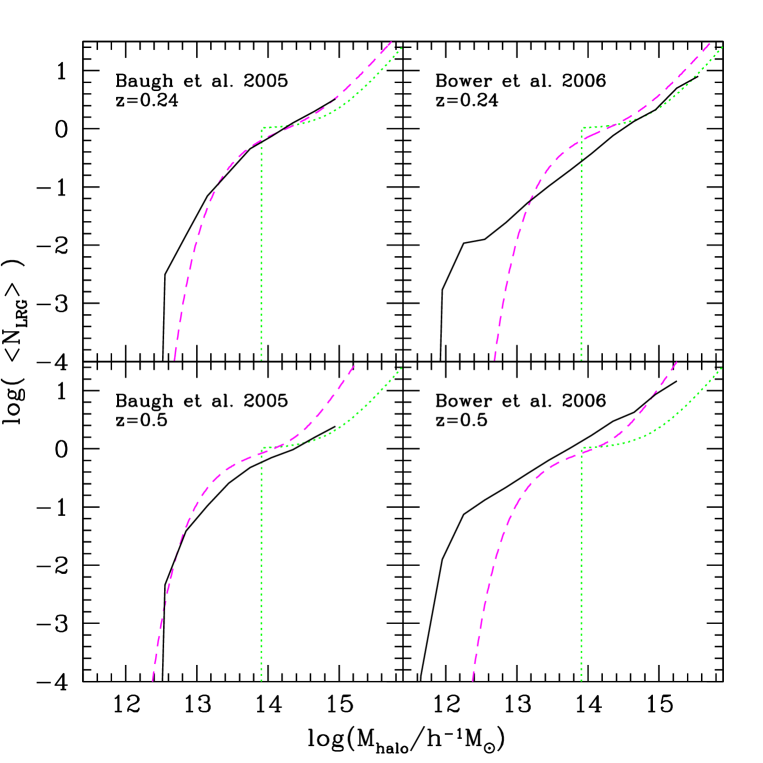
Figure 11: The halo occupation distributions (HOD) of LRGs predicted by the models. The left-hand panels show the predictions for the Baugh et al. model and the right-hand panels for the Bower et al. model. The top row corresponds to $z=0.24$ (SDSS) and the bottom row to $z=0.5$ (2SLAQ). The dotted line shows the HOD fit used by Masjedi et al. to describe SDSS LRGs, and is reproduced in each panel. The dashed lines show the HOD fit to the SDSS and 2SLAQ samples obtained by Wake et al. (2008).

The distribution of halo masses hosting LRGs plotted in Fig. 9 is determined by two factors: the adundance of dark matter haloes, which is a strong function of halo mass for the typical hosts of LRGs, and the number of LRGs which occupy the same dark halo. These factors are separated in Fig. 10, in which we compare the overall mass function of dark haloes with the mass function of haloes weighted by the number of LRGs they contain. The solid lines show the mass function of dark matter haloes, which is determined by the values of the cosmological parameters, the form and amplitude of the power spectrum of matter fluctuations and the redshift (e.g. Governato et al. 1999). The dashed lines show the mass function of haloes multiplied by the average number of LRGs as a function of halo mass. At the mass where the solid and dashed lines cross, these haloes host on average one LRG. At lower masses, the mean number of LRGs per halo rapidly falls below one (this is the ratio of the abundance indicated by the dashed line divided by the abundance shown by the solid line). There is a threshold mass which must be reached before there is any possibility of a halo hosting an LRG. At this mass, only a tiny fraction of haloes actually contain an LRG. Nevertheless, these low mass haloes, because they are much more abundant than the more massive haloes, which have a higher mean number of LRGS, make an important contribution to the overall space density of LRGs. Hence it is essential for a model to take into account the scatter in the formation histories of dark matter haloes in order to accurately model the space density and clustering of LRGs. In the high mass tail of the mass function, the amplitude of the dashed curve exceeds that of the solid curve; at these masses, haloes host more than one LRG. Fig. 10 shows that, at $z=0.24$, in the Baugh et al. model there are an average of $\sim 3$ SDSS LRGs per halo at ${\rm M_{halo}}\approx 1\times 10^{15}\,{\rm h^{-1}M_{\odot}}$. At $z=0.5$, the mass of haloes which host on average one LRG (${\rm M_{halo}}\approx 2.5\times 10^{14}\,{\rm h^{-1}M_{\odot}}$) is higher than at $z=0.24$ and the most massive haloes do not contain as many LRGs as the most massive haloes present at $z=0.24$. This figure also shows that the Bower et al. model predicts a higher mean number of LRGs per halo than the Baugh et al. model at $z=0.5$; for haloes of mass ${\rm M_{halo}}\approx 1\times 10^{15}\,{\rm h^{-1}M_{\odot}}$, the Bower et al. model predicts an average of 10 LRGs per halo. The multiple occupancy of LRGs in high mass haloes has important consequences for the form of the predicted correlation function at small pair separations (i.e. $r<1h^{-1}$Mpc).

Figure 12: The number of times a given number of LRGs is found within a common host halo in the Bower et al. model, in the whole of the Millennium Simulation volume. (Note we do not show haloes with zero LRGs.) The solid and dotted lines show the distributions at $z=0.24$ and $z=0.50$, respectively. Recall that the space density of LRGs selected at $z=0.5$ is greater than that at $z=0.24$. Note that the distribution of occupation numbers at $z=0.50$ extends out to around 30 LRGs per halo.

Figure 13: The two-point correlation function of LRGs in the Bower et al. model. Upper panel: The real-space correlation function at $z=0.24$ (dashed line) and $z=0.50$ (solid line). Also shown in this panel are data from Masjedi et al. (2006) (SDSS LRG sample) and from Ross et al. (2007a) (2SLAQ sample). Lower panel: The redshift-space correlation function, at $z=0.24$ (dashed line) and $z=0.50$ (solid line). For comparison we plot the real-space correlation functions shown in the upper panel using dotted lines. The symbols show the correlation function of LRGs in redshift-space from Zehavi et al. (2005) and Ross et al. (2007a).

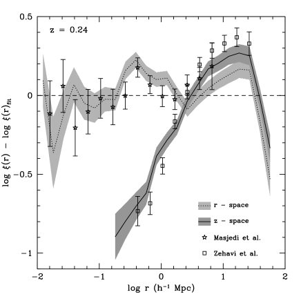
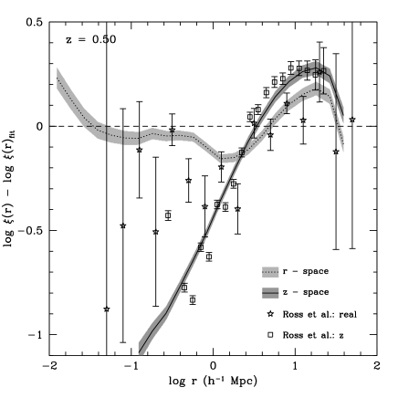
Figure 14: The ratio between the two-point correlation function of LRGs and a power law, $\xi(r)_{\rm fit}=(r/r_{0})^{-2.07}$, where $r_{0}=8.2\,h^{-1}\,{\rm Mpc}$ at $z=0.24$ (upper panel) and $r_{0}=7.1\,h^{-1}\,{\rm Mpc}$ at $z=0.50$ (lower panel). The dotted and solid lines show the predictions of the Bower et al. model in real and redshift-space, respectively. The shaded areas show the $1\sigma$ Poisson errors derived using the number of pairs expected in the model at a given separation.

The mean number of LRGs as a function of halo mass in the halo occupation distribution (HOD), as predicted by GALFORM, is plotted in Fig. 11. For comparison, we also plot the function quoted as a description of the HOD for SDSS LRGs by Masjedi et al. (2006), which is reproduced in each panel of Fig. 11 to serve as a reference point (dotted line). The Masjedi et al. HOD was not derived by fitting the model correlation functions to that measured for LRGs. Instead, this is simply the HOD for the brightest luminosity bin of the main SDSS galaxy sample analyzed by Zehavi et al. (2005). Although galaxies in this sample have similar luminosities and colours to LRGs, they have a different redshift distribution and the selection is only crudely matched. Fig. 11 shows that whilst this parametric form for the HOD is a reasonable match to that predicted by the models for massive haloes with more than 1 LRG, it is a poor description at lower masses. As we have argued before, even though low mass haloes host a mean number of LRGs below unity, there are more of them than there are high mass haloes, so these objects make a significant contribution to the clustering signal (see a similar discussion in Baugh et al. 1999). Ho et al. (2008) estimated the HOD for a sample of LRGs in clusters and found a result similar to the predictions of the Bower et al. model at $z=0.5$. A more detailed modelling of the transition from 1 LRG per halo to 0 LRGs per halo is required to describe the model predictions, such as that advocated by Zheng et al. (2005). Wake et al. (2008) have carried out such a calculation, fixing the background cosmology to match that used in the two models, and Fig. 11 shows that their estimates are in better agreement with the model predictions (Baugh et al. model) than with the HOD advocated by Masjedi et al. (2006; see also Kulkarni et al. 2007). Nevertheless, there are still some discrepancies between the fit obtained by Wake et al. and our model predictions. This could be due to the fact that the models do not reproduce exactly the number density of LRGs, whereas Wake et al. include this as a constraint on their HOD parameters.

We plot the frequency of finding a given number of LRGs within a common dark matter halo in Fig. 12. Here the number of haloes plotted on the y-axis is the number within the full volume of the Millennium simulation ($0.125h^{-3}{\rm Gpc}^{3}$), which contain the specified number of LRGs. At $z=0.5$, nearly ten thousand dark matter haloes in the Millennium contain more than one LRG. Haloes with only one LRG are approximately ten times more common. At the median redshift of the 2SLAQ survey, the tail of haloes with more than one LRG extends to $\sim 30$, reflecting the higher space density of LRGs in this sample compared with the SDSS LRG sample.

Before presenting explicit predictions for the correlation function of LRGs, it is instructive to compute the asymptotic bias factor, $b_{\rm eff}$, which quantifies the boost in the clustering of LRGs relative to that of the underlying matter distribution on large scales ($\xi_{\rm LRG}\approx b^{2}_{\rm eff}\xi_{\rm mass}$). This will allow us to compare the clustering predictions of the Baugh et al. and Bower et al. models. (We cannot make a direct prediction of the correlation function of galaxies in the Baugh et al. model, because, unlike the Bower et al. model, it is not implanted in an N-body simulation.) The asymptotic bias factor can be calculated analytically using the mass function of haloes which host an LRG, $N(z,M^{\prime})$, and the bias as a function of halo mass, $b(M^{\prime},z)$ (e.g. Baugh et al. 1999):

$$b_{\rm eff}(z)=\frac{\int_{M}N(z,M^{\prime})\,b(M^{\prime},z)\,{\rm d}\ln M^{\prime}}{\int_{M}N(z,M^{\prime}){\rm d}\ln M^{\prime}}.$$ (13)

The integrals are over the range of halo masses which host LRGs. The bias factor, $b(M,z)$, for haloes of mass $M$, as a function of redshift is computed using the prescription of Sheth, Mo & Tormen (2001). For the Baugh et al. model we calculate an effective bias of $b_{\rm eff}=2.45$ at $z=0.24$, and $b_{\rm eff}=2.27$ at $z=0.50$. In the case of the Bower et al. model the values are slightly lower, with $b_{\rm eff}=1.82$ at $z=0.24$ and $b_{\rm eff}=1.72$ at $z=0.50$. Using a sample of 35 000 LRGs from the SDSS, Zehavi et al. (2005) measured a bias of $b=1.84\pm 0.11$, which is in agreement with the predictions of the Bower et al. model (see also Kulkarni et al. 2007 and Blake et al. 2007).

For the remainder of this section, we focus on the predictions of the Bower et al. model. As this model is implemented in an N-body simulation, it can be used to produce direct predictions for the spatial distribution of galaxies and hence the two-point correlation function. The published Bower et al. model associates the central (biggest) galaxy in each halo with the largest substructure in the halo. For haloes without resolved substructures, the central galaxy is assigned to the position of the most bound particle. Satellite galaxies are associated with the substructure corresponding to the halo in which they formed or to the most bound particle from the halo in which they formed. Fig. 13 shows the predicted correlation function for this model in real-space and in redshift-space. In real-space, the cartesian co-ordinates of the LRGs within the simulation box are used to compute pair separations. In the redshift-space, galaxy positions along one of the axes are perturbed by the peculiar velocity of the galaxy, scaled by the appropriate value of the Hubble parameter. This corresponds to the distant observer approximation, which is reasonable given the median redshifts of the observational samples. Fig. 13 shows that the correlation functions predicted by the Bower et al. model agree spectacularly well with the measured correlation functions, both in real and redshift space. The agreement between the model predictions and the observational estimates in real-space is particularly noteworthy. The real-space correlation function of LRGs is very close to a power law over three and a half decades in pair separation, varying in amplitude over this range by nearly eight orders of magnitude. The extension of the power-law in the model predictions from $r\sim 1h^{-1}$Mpc down to $r\approx 0.01h^{-1}$Mpc is a remarkable success of the model. The correlation function on these scales is determined by pairs of LRGs within the same dark matter halo. If the model did not predict that some haloes contain more than one LRG, the correlation function would tend to $\xi\sim-1$ on scales smaller than the typical radius of the haloes hosting LRGs (see Benson et al. 2000 for a discussion of this point). The slope of the correlation function on such small scales is a strong test of the model through the predicted number of LRGs per halo.

In the lower panel of Fig. 13, we have retained the same dynamic range on both axes to allow a ready comparison of the clustering signal predicted in redshift-space with that obtained in real-space. To further aid this comparison, we have also reproduced the real-space predictions from the upper panel as dotted lines. The impact of including the contribution of peculiar motions when inferring the distance to galaxies depends on the scale. On intermediate and larger scales($r>3h^{-1}$Mpc), bulk motions of galaxies result in an enhancement in the amplitude of the correlation function measured in redshift-space. This boost is modest because, as we demonstrated above, LRGs are biased tracers of the matter distribution (Kaiser 1987). On small scales, the clustering signal in redshift-space is significantly lower than in real-space. Again, this feature of the predictions, a damping of the clustering on small scales in redshift-space, is expected if the sample contains haloes which host multiple LRGs; the peculiar motions of the LRGs within the halo cause an apparent stretching of the structure in redshift-space, diluting the number of LRG pairs. The clustering predicted in redshift-space agrees extremely well with the measurements by Zehavi et al. (2005) and Ross et al. (2007a).

Another view of the comparison between the predicted and measured correlation functions is presented in Fig. 14, in which we plot the correlation function divided by a reference power law, $\xi(r)_{\rm fit}=\left(r/r_{0}\right)^{\gamma}$. This way of plotting the results emphasizes any differences between model and data by expanding the useful dynamic range plotted on the y-axis. In both panels, for the reference power law we fit a slope of $\gamma=-2.07$, which agrees with the slope inferred for the real-space correlation function by Masjedi et al. (2006). For the correlation lengths in each panel, we use $r_{0}=8.2\,{\rm h^{-1}\,Mpc}$ at $z=0.24$ (upper panel) and $r_{0}=7.1\,{\rm h^{-1}\,Mpc}$ at $z=0.50$ (lower panel). Fig. 14 shows clearly the difference between the shape of the correlation function in real-space and redshift space. The level of agreement between the model predictions and the measurements is impressive, particularly in view of the fact that no model parameters were fine-tuned to achieve this match.

5 The star formation and merger histories of LRGs

Figure 15: Three examples of star formation histories of $z=0.24$ LRGs extracted from the Bower et al. model, plotted as a function of the lookback time from $z=0$. The upper axis gives the corresponding redshift. The star formation rate plotted is the sum of the star formation rate in all of the progenitor galaxies present at a given redshift.

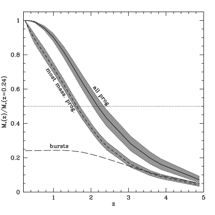
Figure 16: The evolution of the total stellar mass of SDSS LRGs, as predicted by the Bower et al. model. The stellar mass in place at a given redshift is expressed as a fraction of the mean stellar mass of SDSS LRGs at $z=0.24$. The mean fraction of mass in place as a function of lookback time (defined so that $t(z=0)=0$), summed over all progenitors and for the most massive progenitor of the SDSS LRGs, is shown by the solid and short-dashed lines respectively. The shaded region indicates the 1$\sigma$ scatter in this ratio. The long-dashed line shows the fraction of the mean mass accounted for by bursts of star formation, in all progenitors of the $z=0.24$.

Semi-analytical galaxy formation models trace the full star formation and merger histories of galaxies. This allows us to build up a picture of how the stellar mass of LRGs was assembled and how the LRG population changed between the median redshifts of the 2SLAQ and SDSS surveys. The merging history, in particular, has implications for the clustering expected on small scales, which, as we saw in the previous section, is in excellent agreement with the observational estimates (e.g. Masjedi et al. 2006).

We first consider the star formation and mass assembly histories of LRGs. There are two ways in which a galaxy can acquire stellar mass in hierarchical models: 1) through the formation of new stars and 2) through the accretion of pre-existing stars in galaxy mergers (Baugh, Cole & Frenk 1996; Kauffmann 1996). A nice discussion of the relative importance of these two processes for brightest cluster galaxies can be found in de Lucia & Blaizot (2007).

In Fig. 15 we show some examples of star formation histories for three $z=0.24$ LRGs in the Bower et al. model. The star formation rate plotted is the sum of the star formation rate over all of the progenitor galaxies at each redshift. The star formation history contains contributions from quiescent star formation in galactic disks and from starbursts triggered by galaxy mergers or dynamically unstable disks in the case of the Bower et all. model. In general, the galaxy star formation histories predicted by hierarchical models tend to be more complex than the simple, one parameter, exponentially declining models typically considered in the literature (for some examples of star formation histories generated by semi-analytical models, see Baugh 2006). Fig. 15 confirms that the LRG selection isolates a subset of galaxies in the model with more passive star formation histories, which are closer to exponential models (though these examples still display significant structure in their star formation histories at high redshift). The three examples have similar forms, with a peak at a lookback time $10\la t\la 12$ Gyrs, followed by a smooth decay. In one of the examples, plotted with the dotted line, there is still appreciable star formation at $z=0.24$. Around 5% of LRGs in the Bower et al. model display star formation rates at $z=0.24$ in excess of $0.1\,{\rm M_{\odot}\,h^{-2}\,yr^{-1}}$, with the largest being $30\,{\rm M_{\odot}\,h^{-2}\,yr^{-1}}$. These low star formation rates indicate that for the bulk of LRGs in the model, ongoing star formation is not an important channel for increasing the stellar mass of LRGs, given the large stellar masses predicted for these galaxies.

The evolution of the stellar mass of LRGs with redshift is shown in Fig. 16. In this plot, we take LRGs of similar stellar mass at $z=0.24$ from the Bower et al model and track the build up of their stellar mass with redshift. The solid line shows how the mean stellar mass of the sample of LRGs builds up over time, expressed as a fraction of the mean mass of the LRGs at $z=0.24$. Here we sum over all the progenitors of SDSS LRGs. Half of the stellar mass of the $z=0.24$ LRGs was already in place at $z=2.2$. The mean change in stellar mass since $z=0.5$ is around $1\%$. If, instead, we consider only the most massive progenitor, the figure reveals that half of the mass was already in one object at $z=1.6$. Since $z=0.5$, the mean fractional change in stellar mass of the biggest progenitor is just over 0.1; since $z\sim 1$, the average stellar mass has grown by only 25%. This evolution is in agreement with estimates inferred from the observed evolution of the luminosity function for a matched sample of LRGs (i.e. by considering the subset of 2SLAQ LRGs which have similar properties to the SDSS LRGs; Wake et al. 2006). Fig. 16 also shows the contribution to the stellar mass of LRGs from bursts of star formation initiated by galaxy mergers or by the formation of bars in dynamically unstable discs. In total, this channel of star formation is only responsible for around $30\%$ of the stellar mass of SDSS LRGs. Furthermore, the level of contribution from this mode of star formation has changed little since a redshift of $z\sim 1.5$. This reflects the general trend for mergers to become more gas poor ( or “dry”) with declining redshift in hierarchical models, due to the increasing consumption of gas by quiescent star formation in galactic discs, and the overall decline in the merger rate towards the present day. Given the relatively small star formation rates predicted in model LRGs since $z\sim 1$, the steady increase in the stellar mass of LRGs over the redshift interval $z=1$ to $z=0.24$ is driven primarily by gas-poor galaxy mergers, which reassemble pre-formed stars.

We now look in more detail at how SDSS LRGs build up their mass in galaxy mergers. The number of progenitor galaxies depends upon whether or not a mass cut is applied before a progenitor is counted. If a mass cut is not used, the number of progenitors obtained is likley to be dominated by low mass galaxies, which only bring in a small fraction of the galaxy’s mass. Masjedi et al. (2006) used their measurement of the correlation function on small scales to constrain a simple model for mergers between LRGs, prior to the median redshift of the SDSS sample. Here we do not attempt to consider only those progenitors which are matched to the SDSS sample selection. Instead, we consider progenitors at $z=0.5$ which account for 30% of more of the stellar mass of the SDSS LRG at $z=0.24$. We then further distinguish between progenitors which satisfy the 2SLAQ selection and those that do not.

Table 4 shows the number of progenitors of SDSS LRGs predicted by the Bower et al model. The first row gives the percentage of SDSS LRGs which have 0,1,2 or 3 progenitors at $z=0.5$ which each account for 30% or more of the mass of the $z=0.24$ LRG. Typically, in the model, SDSS LRGs have one such progenitor at $z=0.5$. Only 11% of LRGs have more than one progenitor which represents 30% or more of the mass. In the case where a SDSS LRG has only one progenitor with $\geq 30\%$ of the mass, then in 70% of cases this progenitor will be a 2SLAQ LRG. When there are two sizeable progenitors present at $z=0.5$, then in half of the cases, one galaxy is a 2SLAQ LRG and the other progenitor fails to meet the 2SLAQ LRG definition. In around one third of cases, both progenitors are LRGs.

# progenitors $>30\%$ mass	0	1	2	3
(%)	0.3	88.6	11.0	0.1
# progenitors $>30\%$ mass
and 2SLAQ LRG
0	100	27	10	29
1	-	73	55	29
2	-	-	35	29
3	-	-	-	13

Table 4: The nature of the progenitors of SDSS LRGs in the Bower et al. (2006) model. The progenitor galaxies are identified at $z=0.5$ and by definition are required to account for at least 30% of the stellar mass of the LRG at $z=0.24$, the median redshift of the SDSS sample. The second row gives the percentage of SDSS LRGs with 0, 1, 2 and 3 such progenitors. The rows give the percentage of cases in which a galaxy has the stated number of progenitors which themselves satisfy the LRG selection criteria at $z=0.5$.

6 Discussion and conclusions

In this paper we have extended the tests of hierarchical galaxy formation models to include predictions for the properties of a special subset of the galaxy population called luminous red galaxies (LRGs). Given their rarity, bright luminosities and extreme colours, LRGs represent a stern challenge for the models. They are particularly interesting from the point of view of developing the model physics, since the abundance and nature of LRGs probes precisely the regime in which the models are currently most uncertain, the formation of massive galaxies. Historically, hierarchical models have tended to overproduce bright galaxies at the present day (see Baugh 2006). The phenomena invoked to restrict the growth of large galaxies locally, naturally, have an impact on the form of the bright end of the galaxy luminosity function at intermediate and high redshifts, where LRGs dominate. In addition, LRGs have the red colours expected of a passively evolving stellar population, which restricts the range of possible star formation histories for these galaxies.

It may appear odd to talk about producing model predictions after an observational dataset has been constructed. The models considered in this paper contain parameters whose values were fixed by requiring them to reproduce a subset of the data available for the local galaxy population (for a discussion see Cole et al. 2000). None of the datasets used for this purpose make explicit reference to the redshifts of interest for the LRG surveys discussed here, nor were red galaxies singled out for special attention in the process of setting the model parameters. We do, however, require that our semi-analytical models reproduce as closely as possible the bright end of the present day luminosity function of all galaxies, which does tend to be dominated by red galaxies with passive stellar populations (e.g. Norberg et al. 2002). Therefore, by comparing the models to the observed properties of the LRG population, we are in effect testing the physics which govern the evolution of the bright end of the luminosity function, as traced by objects with the special colours of LRGs.

The two models considered, Baugh et al. (2005) and Bower et al. (2006), enjoy a considerable number of successes and, inevitably, have some shortcomings (see Section 2). It is important to be clear that in this paper, we have not adjusted or tinkered with any of the parameters of the published models in order to improve the comparison of the model output with the observational data. This “warts and all” exercise illustrates the appeal of the semi-analytical approach, in that a given model yields a broad range of outputs which are directly testable against observations. In both models, LRGs are predominantly bulge dominated galaxies (although 20-40% are expected to be spirals with old stellar populations), with velocity dispersions of $\sigma\sim 320{\rm kms}^{-1}$ and stellar masses around $1-2\times 10^{11}h^{-1}M_{\odot}$, which is higher than observed. The models give different predictions for the radii of LRGs, with the Baugh et al model predicting the larger LRGs. Both models fail to produce bright spheroids that are large enough to match the locally observed radius-luminosity relation (see Almeida et al. 2007 for a discussion of how the sizes of spheroids are computed in the models and for possible solutions to this problem).

The Baugh et al. and Bower et al. models are two feasible simulations of the galaxy formation process, which differ in several ways, as we reviewed in Section 2 (see also the comparison in Almeida et al. 2007). A key difference between the models, in terms of the analysis presented in this paper, is the form of the physics invoked to quench the formation of massive galaxies. In both models the amount of gas cooling from the hot halo, to provide the raw material for star formation, is reduced by quite different means. Baugh et al. invoke a wind which expels cold gas from intermediate mass haloes. This gas is assumed to be ejected with such vigour that it does not get recaptured by more massive haloes in the merger hierarchy. Hence, in this model, the more massive haloes contain fewer baryons than expected from the universal baryon fraction, and therefore less gas is available to cool from the hot halo. One controversial aspect of this scheme is the energy source required to drive the wind. Benson et al. (2003) showed that the energy produced by supernova explosions is unlikely to be sufficient to power a wind of the strength required to reproduce the sharpness of the break in the local galaxy luminosity function, and argued that the accretion of gas onto a central supermassive black hole could be the solution. Bower et al. invoked an AGN feedback model in which the luminosity of the AGN heats the hot halo (see also Croton et al. 2006; see Granato et al. 2004 for an alternative model). This suppresses the cooling flow in massive haloes which have quasi-static hot gas atmospheres.

The predictions of the Baugh et al. and Bower et al. models bracket the observed luminosity function of LRGs, with the Bower et al. model giving the better overall agreement with the SDSS and 2SLAQ results. The shape and normalization of the z=0.24 LRG luminosity function predicted by the Bower et al. model are in excellent agreement with the observations. This is remarkable when one bears in mind that LRGs are an order of magnitude less common than $L_{*}$ galaxies. The Baugh et al. model on the other hand, whilst predicting a similar number density of LRGs, gives a poor match to the shape of the observed luminosity function. At $z=0.5$, the agreement is less good, with the predictions only coming within a factor of 2 of the observed abundance. This implies that the models may not be tracking the evolution of the bright end of the luminosity function accurately over such a large lookback time (40% of the age of the universe), at least for galaxies matching the 2SLAQ selection. Whilst this discrepancy suggests that there are problems modelling the evolution of the red galaxy luminosity function, it is important to note that the Bower et al. model does give a good match to the inferred evolution of the stellar mass function, to much higher redshifts than that of the 2SLAQ sample. We investigated whether it was possible to tune the predictions of the Baugh et al. model to better match the LRG luminosity function; this exercise proved to be unsuccessful suggesting that a more substantial revision to the ingredients of this model, involving further suppression of gas cooling in massive haloes, is required.

Semi-analytical models predict the star formation histories of galaxies, based upon the mass of cold gas which accumulates through cooling and galaxy mergers, and a prescription for computing an instantaneous star formation timescale (examples of star formation histories extracted from the models are given in Baugh 2006). As expected, the stellar populations of model LRGs are old, with luminosity weighted ages in the region of 4-8 Gyr for the SDSS selection, with the Bower et al. model returning the more elderly stars (similar results were reported by de Lucia et al. 2006 and Croton et al. 2006 for massive elliptical galaxies). The semi-analytical model can track the build-up of the stellar mass of LRGs, considering all of the progenitor galaxies. There is little recent star formation in any of the progenitor galaxies of SDSS LRGs; averaging over all progenitors, typically 50% of the $z=0.24$ stellar mass of the LRG has already formed by a redshift of $z\sim 2.2$. However the mass of the main progenitor branch is still growing over this redshift interval. Around half of the mass in the biggest progenitor is put in place since $z\sim 1.5$ through galaxy mergers of ready-made stellar fragments (for a discussion of the difference between the formation time of the stars and the assembly time of the stellar mass, see de Lucia & Blaizot 2007). On average, only 25% of the stellar mass of the LRG is added after $z\sim 1$, in line with observational estimates of the evolution of the stellar mass function, which indicate that many of the most massive galaxies are already in place by $z\sim 1$ (e.g. Bauer et al. 2005; Bundy, Ellis & Conselice 2005; Wake et al. 2006).

Perhaps the most spectacularly successful model prediction is for the clustering of LRGs. Masjedi et al. (2006) estimated the two-point correlation function of SDSS LRGs in real space, free from the distortions in the clustering pattern induced by the peculiar motions of galaxies. These authors found that the real-space correlation function of LRGs is a power law over three and a half decades in pair separation, down to scales of $r\approx 0.01h^{-1}{\rm Mpc}$. Masjedi et al. argued that current halo occupation distribution models could not reproduce such a steep correlation function on small scales because these models asume that galaxies trace the density profile of the dark matter halo, which is shallower than the observed correlation function. This line of reasoning is spurious, as HODs can produce realizations of the two-point correlation function with different small-scale slopes for different galaxy samples, even when the different samples trace the dark matter (see, for example, Figure 22 of Berlind et al. 2003 which compares the correlation functions of old and young galaxies). The small scale slope depends on the interplay between two factors: the number of galaxies within a dark matter halo and the range of halo masses which contain more than one galaxy (e.g. Benson et al. 2000). The Bower et al. model can readily produce predictions of galaxy clustering down to such small scales since it is embedded in the Millennium simulation (Springel et al. 2005). The correlation function predicted by the Bower et al. model agrees impressively well with the observational estimate by Masjedi et al. The HOD used by Masjedi et al. is actually a poor description of the HOD predicted in the Bower et al. model. Further support for the number of LRGs predicted as a function of halo mass comes from the degree of damping of the correlation function seen on small scales in redshift-space. The virialized motions of LRGs within a common halo gives a contribution to the peculiar velocity of these galaxies, which results in the structure appearing stretched when the distance to the LRG is inferred from its redshift. This damping would not be apparent in the case of a maximum of one LRG per halo.

Overall, the agreement between the model predictions and the observation of LRGs is encouraging, demonstrating the true predictive power of semi-analytical models. The two models we have tested have quite different mechanisms to regulate the formation of massive galaxies, with the Bower et al. model invoking “AGN feedback” and the Baugh et al. model relying on a “superwind”; in the former, the raw material for star formation is prevented from cooling in the first place in massive haloes, whilst in the latter cold gas is expelled from the halo before it can form stars. The Bower et al. model does the best in terms of matching the abundance of LRGs, particularly at $z=0.24$. This success is repeated for extremely red objects (EROs) at higher redshifts than the samples considered here, as presented by González-Pérez et al. (in preparation). The Baugh et al. model does less well at reproducing the number of LRGs and EROs. Whilst problems remain in predicting the radii of spheroids and the precise evolution of LRG luminosity function, it is clear that these objects can be accommodated in hierarchical models.

ACKNOWLEDGEMENTS

C. A. gratefully acknowledges support in the form of a scholarship from the Science and Technology Foundation (FCT), Portugal. CMB is supported by the Royal Society. AJB acknowledges support from the Gordon and Betty Moore Foundation. This work was supported in part by a rolling grant from PPARC. We thank the referee for providing a detailed and helpful report. We acknowledge comments and suggestions from Bob Nichol, Nic Ross and Donald Schneider, and the contributions of Shaun Cole, Carlos Frenk, John Helly and Rowena Malbon to the development of the GALFORM code.

References

- Adelberger et al. (2003) Adelberger K.L., Steidel C.C., Shapley A.E., Pettini M., 2003, ApJ, 584, 45
- Almeida et al. (2007) Almeida C., Baugh C.M., Lacey C.G., 2007, MNRAS, 376, 1711
- Barber et al. (2007) Barber T., Meiksin A., Murphy T., 2007, MNRAS, 377, 787
- Bauer et al. (2005) Bauer A.E., Drory N., Hill G.J., Feulner G., 2005, ApJ, 621, L89
- Baugh (2006) Baugh C.M., 2006, Rep. Prog. Physics, 69, 3101
- Baugh et al. (2005) Baugh C.M., Lacey C.G., Frenk C.S., Granato G.L., Silva L., Bressan A., Benson A.J., Cole S., 2005, MNRAS, 356, 1191
- Baugh et al. (1999) Baugh C.M., Benson A.J., Cole S., Frenk C.S., Lacey C.G., 1999, MNRAS, 305, L21
- Baugh, Cole & Frenk (1996) Baugh C.M., Cole S., Frenk C.S., 1996, MNRAS, 283, 1361
- Benson et al. (2003) Benson A.J., Bower R.G., Frenk C.S., Lacey C.G., Baugh C.M., Cole S., 2003, ApJ, 599, 38
- Benson et al. (2000) Benson A.J., Baugh C.M., Cole S., Frenk C.S., Lacey C.G., 2000, MNRAS, 316, 107
- Berlind et al. (2003) Berlind A.A., et al., 2003, ApJ, 593, 1
- Bernardi et al. (2005) Bernardi M., Sheth R.K., Nichol R.C., Schneider D.P., Brinkmann J., 2005, AJ, 129, 61
- Blake et al. (2007) Blake C., Collister A., Lahav O., 2007, MNRAS, accepted, arXiv:0704.3377
- Bower et al. (2006) Bower R.G., Benson A.J., Malbon R., Helly J.C., Frenk C.S., Baugh C.M., Cole S., Lacey C.G., 2006, MNRAS, 370, 645
- Bower et al. (2001) Bower R.G., Benson A.J., Lacey C.G., Baugh C.M., Cole S., Frenk C.S., 2001, MNRAS, 325, 497
- Bower et al. (2007) Brown M.J.I., et al., 2007, ApJ, 654, 858
- Bruzual & Charlot (2003) Bruzual G., Charlot S., 2003, MNRAS, 344, 1000
- Bundy, Ellis & Conselice (2005) Bundy K., Ellis R.S., Conselice C.J., 2005, ApJ, 625, 621.
- Cannon et al. (2006) Cannon R., et al., 2006, MNRAS, 372, 425
- Cole et al. (2000) Cole S., Lacey C.G., Baugh C.M., Frenk C.S., 2000, MNRAS, 319, 168
- Cole et al. (1994) Cole S., Aragon-Salamanca A., Frenk C.S., Navarro J.F., Zepf S.E., 1994, MNRAS, 271, 781
- Conroy et al. (2007) Conroy C., Ho S., White M., 2007, MNRAS, 379, 1491
- Cooray & Sheth (2002) Cooray A., Sheth R., 2002, PhR, 372, 1
- Croton et al. (2006) Croton D.J., et al., 2006, MNRAS, 365, 11
- De Lucia & Blaizot (2007) De Lucia G., Blaizot J., 2007, MNRAS, 375, 2
- De Lucia et al. (2006) De Lucia G., Springel V., White S.D.M., Croton D., Kauffmann G., 2006, MNRAS, 366, 499
- Eisenstein et al. (2005) Eisenstein D.J., et al., 2005, ApJ, 633, 560
- Eisenstein et al. (2001) Eisenstein D.J., et al., 2001, AJ, 122, 2267
- Fabian et al. (2002) Fabian A.C., Voigt L.M., Morris R.G., 2002, MNRAS, 335, 71
- Fukugita et al. (1996) Fukugita M., Ichikawa T., Gunn J.E., Doi M., Shimasaku K., Schneider D.P., 1996, AJ, 111, 1748
- Gallazzi et al. (2006) Gallazzi A., Charlot S., Brinchmann J., White S.D.M., 2006, MNRAS, 370, 1106
- Governato et al. (1999) Governato F., Babul A., Quinn T., Tozzi P., Baugh C.M., Katz N., Lake G., 1999, MNRAS, 307, 949
- Granato et al. (2004) Granato G.L., De Zotti G., Silva L., Bressan A., Danese L., 2004, ApJ, 600, 580
- Helly et al. (2003) Helly J.C., Cole S., Frenk C.S., Baugh C.M., Benson A.J., Lacey C.G., 2003, MNRAS, 338, 903
- Ho et al. (2008) Ho S., Lin Y., Spergel D., Hirata C.M., 2008, arXiv0706.0727
- Hopkins et al. (2006) Hopkins P.F., Hernquist L., Cox T.J., Robertson B., Springel V., 2006, ApJS, 163, 50
- Hütsi (2001) Hütsi G., 2006, A&A, 459, 375
- Kaiser (1987) Kaiser N., 1987, MNRAS, 227, 1
- Kauffmann (1996) Kauffmann G., 1996, MNRAS, 281, 487
- Kauffmann et al. (1993) Kauffmann G., White S.D.M., Guiderdoni B., 1993, MNRAS, 264, 201
- Kennicutt (1993) Kennicutt R.C., 1993, ApJ, 272, 54
- Kulkarni (2007) Kulkarni G.V., Nichol R.C., Sheth R.K., Seo H., Eisenstein D.J., Gray A., 2007, MNRAS, 378, 1196
- Lacey et al. (2008) Lacey C.G., Baugh C.M., Frenk C.S., Silva L., Granato G.L., Bressan A., 2008, MNRAS, in press, arXiv:0704.1562
- Le Delliou et al. (2006) Le Delliou M., Lacey C.G., Baugh C.M., Morris S.L., 2006, MNRAS, 365, 712
- Le Delliou et al. (2005) Le Delliou M., Lacey C.G., Baugh C.M., Guiderdoni B., Bacon R., Courtois H., Sousbie T., Morris S.L., 2005, MNRAS, 357, 11
- Mandelbaum et al. (2006) Mandelbaum R., Seljak U., Cool R.J., Blanton M., Hirata C.M., Brinkmann J., 2006, MNRAS, 372, 758
- Malbon et al. (2007) Malbon R.K., Baugh C.M., Frenk C.S., Lacey C.G., 2007, MNRAS, 382, 1394
- Maller & Bullock (2004) Maller A.H., Bullock J.S., 2004, MNRAS, 355, 694
- Masjedi et al. (2006) Masjedi M., et al., 2006, ApJ, 644, 54
- McCarthy et al. 2007 (2007) McCarthy I.G., et al. 2007, MNRAS, 376, 497
- Nagashima et al. (2005a) Nagashima M., Lacey C.G., Baugh C,M., Frenk C,S., Cole S, 2005a, MNRAS, 358, 1247
- Nagashima et al. (2005b) Nagashima M., Lacey C.G., Okamoto T., Baugh C.M., Frenk C.S., Cole S., 2005b, MNRAS, 363, 31
- Navarro, Frenk & White (1997) Navarro J.F., Frenk C.S., White S.D.M., 1997, ApJ, 490, 493
- Norberg et al. (2002) Norberg P., et al. 2002, MNRAS, 332, 827
- Padmanabhan et al. (2007) Padmanabhan N., et al., 2007, MNRAS, 378, 852
- Peacock & Smith (2000) Peacock J.A., Smith R.E., 2000, MNRAS, 318, 1144
- Roseboom et al. (2005) Roseboom I.G., et al., 2006, MNRAS, 373, 349
- Ross et al. (2007a) Ross N., et al., 2007a, MNRAS, 381, 573
- Ross et al. (2007b) Ross N., Shanks T., Cannon R.D., Wake D.A., Sharp R.G., Croom S.M., Peacock J.A., 2007b, MNRAS submitted, arXiv0704.3739
- Seljak (2000) Seljak U., 2000, MNRAS, 318, 203
- Sheth, Mo & Tormen (2000) Sheth R.K., Mo H.J., Tormen G., 2000, MNRAS, 323, 1
- Simien & de Vaucouleurs (1986) Simien F., de Vaucouleurs G., 1986, ApJ, 302, 564
- Springel et al. (2005) Springel V., et al., 2005, Nature, 435, 629
- Trager et al. (2000) Trager S.C., Faber S.M., Worthey G., González J.J., 2000, AJ, 119, 1645
- Wake et al. (2006) Wake D.A., Nichol R.C., et al., 2006, MNRAS, 372, 537
- Wake et al. (2008) Wake D.A., Sheth R.K., Nichol R.C., et al. 2008, submitted
- Wilman et al. (2005) Wilman R.J., Gerssen J., Bower R.G., Morris S.L., Bacon R., de Zeeuw P.T., Davies R.L., 2005, Nature, 436, 227
- White & Frenk (1991) White S.D.M., Frenk C.S., 1991, ApJ, 379, 52
- York et al. (2000) York D.G., et al., 2000, AJ, 120, 1579
- Zehavi et al. (2005) Zehavi I., et al., 2005, ApJ, 621, 22
- Zheng et al. (2005) Zheng Z., et al., 2005, ApJ, 633, 791
- (72)