A Simple Probabilistic Algorithm for Detecting Community Structure in Social Networks

Abstract

With the growing number of available social and biological networks, the problem of detecting network community structure is becoming more and more important which acts as the first step to analyze these data. The community structure is generally regarded as that nodes in the same community tend to have more edges and less if they are in different communities. We come up with SPAEM, a Simple Probabilistic Algorithm for detecting community structure which employs E-M(Expectation-Maximization) algorithm. We also give a criterion based on minimum description length to identify the optimal number of communities. SPAEM can detect overlapping nodes and handle weighted networks. It turns out to be powerful and effective by testing simulation data and some widely known data sets.

I INTRODUCTION

Many systems can be represented by networks where nodes denote entities and links denote existing relation between nodes, such systems may include the web networks Freeman (1992), the biological networks LH et al. (1999), ecological web Lusseau et al. (2003) and social organization networks Zachary (1977). Many interesting properties have also been identified in these networks such as small worldWatts (1998) and power law distribution A-L and R (1999), one property that attracts much attention is the network community structure, which is the phenomenon that nodes within the same community are more densely connected than those in different communities Girvan and Newman (2002). It is important in the sense that we can get a better understanding about the network structure.

This problem has been studied by researchers from different perspectives. Earlier approaches for identifying communities could be divided into two categories: the hierarchical approach and divisive approach. The former merged two closest nodes into one community recursively until the whole network became one single community and the latter worked from the top to bottom which split the whole network into 2 communities recursively until every node was a community. These algorithms usually needed a measure to evaluate the closeness or dissimilarity between two nodes, see Girvan and Newman (2002); Luo et al. (2007); Zhou (2003); Radicchi et al. (2004); Zhang et al. (2007a).

An important modularity measure for evaluating the goodness of community structure was proposed by Newman Newman and Girvan (2004) and several algorithms worked by maximizing it Newman (2006a, b); White and Smyth (2005); Duch and Arenas (2005). This measure was very efficient in characterizing community structure for networks with balanced structure, however, the internal scale problem in its definition Fortunato and Barth lemy (2007) made it fail to work well for unbalanced networks such as those whose communities varied in size and degree sequence. Quite recently, an information based algorithm by Martin Rosvall and Bergstrom (2007) could accurately resolve communities and in particular can to some extent get over the scale problem of modularity.

Also, researchers Palla et al. (2005) found that communities were overlapping rather than disjoint, subsequent algorithms Zhang et al. (2006); Rosvall and Bergstrom (2007); Zhang et al. (2007b) were designed to deal with overlapping communities. A mixture model by Newman Newman and Leicht (2007) could automatically detect patterns inside a network, meanwhile, it was able to detect overlapping nodes as a byproduct.

All these state-of-art algorithms motivate us to treat the community detection problem as a probabilistic inference problem, we should mine the internal information which determines the network topology. These internal information gives insight to the network structure. Our work is inspired by probabilistic latent semantic analysis Hofmann (2001) which is a powerful algorithm in text ming, it models that a term occurs in a document if they are under the same latent topic. This idea is employed here to detect community structure in complex networks.

II METHOD

Assume that the network considered is undirected and unweighted with $n$ nodes, let $A$ denote the adjacent matrix and $N(i)$ the neighbors of node $i$. Assume that two nodes $i$ and $j$ have an edge if they belong to the same community, which is hidden information, see FIG 1. According to the model, community membership $g_{ij}$ can be assigned to edge $e_{ij}$, such that $g_{ij}=r$ if and only if two nodes of edge $e_{ij}$ belong to community $r$.

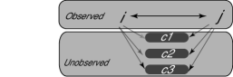
Figure 1: An observed edge exists between nodes $i,j$ due to the fact that they participate in the same community, which is hidden or unobserved information. Our model mines these hidden information such that they generate the network with the highest probability.

Suppose $c$ communities are to be detected, let $\pi_{r}$ be the probability of community $r$, which can be viewed as the fraction of nodes in community $r,r=1,2,...,c$. The conditional probability $Pr(i|r)$ of node $i$ appearing in community $r$, denoted by $\beta_{r,i}$, satisfies $\sum_{i=1}^{n}\beta_{r,i}=1$. In fact $\beta_{r,i}$ can be viewed as the importance of node $i$ in community $r$, the larger the value of $\beta_{r,i}$ is, the more important node $i$ is in community $r$. Let $\pi$ and $\beta$ denote set of parameters $\{\pi_{r},r=1,2,...,c\}$ and $\{\beta_{r,i},r=1,2,..,c,i=1,2,...,n\}$, respectively.

Naturally, the probability of edge $e_{ij}$ existing and belonging to community $r$ is modeled as

$$Pr(e_{ij},g_{ij}=r|\pi,\beta)=\pi_{r}\beta_{r,i}\beta_{r,j}$$

In fact, $Pr(e_{ij},g_{ij}=r|\pi,\beta)$ can be viewed as the contribution of community $r$ to the formation of edge $e_{ij}$. Then probability $Pr(e_{ij}|\pi,\beta)$ of the existence of edge $e_{i,j}$ is the sum of contribution from all communities $r=1,2,..,c$, namely

$$Pr(e_{ij}|\pi,\beta)=\sum_{r=1}^{c}Pr(e_{ij},g_{ij}=r|\pi,\beta)=\sum_{r=1}^{c}\pi_{r}\beta_{r,i}\beta_{r,j}$$

The observed information is the edge $e_{ij}$, however, it’s determined by the unobserved parameters $\pi,\beta$, so these unobserved parameters $\pi,\beta$ determine the network topology $A$, this is exactly the idea depicted in FIG 1.

Next, the log probability of network $A$ under parameters $\pi,\beta$ can be modeled as

$$LL =\log Pr(A|\pi,\beta)=\sum_{i=1}^{n}\sum_{j:j\in N(i)}\log Pr(e_{ij}|\pi,\beta)$$ (1)

$$=\sum_{i=1}^{n}\sum_{j:j\in N(i)}\log(\sum_{r=1}^{c}\pi_{r}\beta_{r,i}\beta_{r,j})$$

Parameters $\pi,\beta$ should be estimated to maximize Eq(1). However, $LL$ in Eq(1) contains log of sums and is difficult to optimize but can be optimized easily by Expectation-Maximization algorithm.

II.1 The EM Formula

The EM algorithm is proposed to maximize probability that contains latent variables Dempster et al. (1977), it computes the posterior probability of the latent variables under the observed data and currently estimated parameters in the E-step and updates parameters with these posterior probabilities in the M-step. The posterior probability $Pr(g_{ij}=r|A,\pi,\beta)$ of edge $e_{i,j}$ belonging to community $r$ under the observed network $A$ and parameter $\pi,\theta$, denote this probability by $q_{ij,r}$, then

$$q_{ij,r}=Pr(g_{ij}=r|A,\pi,\beta)=\frac{Pr(g_{ij}=r,A|\pi,\beta)}{Pr(A|\pi,\beta)}$$

$$=\frac{Pr(e_{ij},g_{ij}=r,A|\pi,\beta)}{Pr(A|\pi,\beta)}$$

by simple deduction the E-step formula can be obtained:

$$q_{ij,r}=Pr(g_{ij}=r|A,\pi,\beta)=\frac{\pi_{r}\beta_{r,i}\beta_{r,j}}{\sum_{s=1}^{c}\pi_{s}\beta_{s,i}\beta_{s,j}}$$ (2)

In fact, $q_{ij,r}$ is the fraction of contribution from community $r$ under the observed matrix $A$ and parameters $\pi,\beta$. Obviously, the expected log-probability of the network is

$$\overrightarrow{LL}=\sum_{i=1}^{n}\sum_{j:j\in N(i)}\sum_{r=1}^{c}q_{ij,r}\ln Pr(e_{i,j},g_{ij}=r|\pi,\beta)$$

$$=\sum_{i=1}^{n}\sum_{j:j\in N(i)}\sum_{r=1}^{c}q_{ij,r}\ln(\pi_{r}\beta_{r,i}\beta_{r,j})$$ (3)

Combining with the constraints that $\sum_{r}\pi_{r}=1,\sum_{i=1}^{n}\beta_{r,i}=1,r=1,2,..,c$, the lagrange form of $\overrightarrow{LL}$ is:

$$L=\sum_{i=1}^{n}\sum_{j:j\in N(i)}\sum_{r=1}^{c}q_{ij,r}\ln(\pi_{r}\beta_{r,i}\beta_{r,j})$$

$$+\alpha(\sum_{r=1}^{c}\pi_{r}-1)+\sum_{r=1}^{c}\gamma_{r}(\sum_{i=1}^{n}\beta_{r,i}-1)$$ (4)

where $\alpha,\gamma_{r},r=1,2,...,c$ are lagrange multipliers. The derivatives of $L$ in Eq(II.1) are:

$$\frac{\partial L}{\partial\pi_{r}}=\sum_{i=1}^{n}\sum_{j:j\in N(i)}q_{ij,r}+\alpha$$ (5)

$$\frac{\partial L}{\partial\beta_{r,i}}=\sum_{j:j\in N(i)}q_{ij,r}+\gamma_{r}$$ (6)

By setting the derivative in Eq(5),Eq(6) to zero and combining the constraints $\sum_{r}\pi_{r}=1,\sum_{i=1}^{n}\beta_{r,i}=1,r=1,2,..,c$, the M-step formulas are:

$$\pi_{r} =\frac{\sum_{i}\sum_{j:j\in N(i)}q_{ij,r}}{\sum_{i}\sum_{j:\in N(i)}\sum_{s=1}^{c}q_{ij,s}}$$ (7)

$$\beta_{r,i} =\frac{\sum_{j:j\in N(i)}q_{ij,r}}{\sum_{k=1}^{n}\sum_{j:j\in N(k)}q_{kj,r}}$$ (8)

In the E-step, the membership of an edge is influenced by its nodes while in the M-step, the node importance in communities is influenced by the membership of all its links. By iterating E-steps and M-steps, $LL$ in Eq(1) will increase.

Once all the parameters are estimated, the preference of node $i$ belonging to community $s$ is computed as $u_{s,i}=\pi_{s}\beta_{s,i}$, and node $i$ is assigned to community $r$ such that $r=argmax_{s}\{u_{s,i}=\pi_{s}\beta_{s,i},s=1,2,..,r\}.$ $u_{s,i}$s can be normalized so that their sum is 1 to comply with probability normalization condition . In fact, this gives a soft assignment and can be used to detect overlapping nodes. Suppose for node $i$, $r=argmax_{s}\{u_{s,i}=\pi_{s}\beta_{s,i},s=1,2,..,r\}$, empirically node $i$ is an overlapping node if there is another community $s$ such that $\frac{u_{s,i}}{u_{r,i}}>1/10$.

Parameters $\pi,\beta$ are initialized with random values and iterated using E-step and M-step until $LL$ stabilizes. To avoid the algorithm getting stuck in a local maxima, we adopt restart strategy which runs the EM algorithm several times with different initial parameter values.

Suppose the network has totally $l$ edges, obvious the algorithm has a linear time complexity $O(cl)$, which makes it an appealing approach for detecting large scale networks. Note that the actual running time is also relevant to the number of EM iterations and the number of restarts. We name our model SPAEM for easier representation, abbreviation for Simple Probabilistic Algorithm which employs the idea of Expectation and Maximization framework.

II.2 Model Selection Issue

SPAEM needs a pre-specified community number $c$ and this is regarded as prior knowledge. However, the determination of $c$ is a non-trivial task and is difficult when no prior knowledge can be obtained. We try to handle it using Minimum Description Length principle Rissanen (1978).

In general, $LL$ in Eq(1) increases as $c$ increases, meanwhile, an extra cost has to be paid for due to the increase in the number of parameters $K=(c-1)+c(n-1)$. There should be some balance between $LL$ and $K$, and the idea of minimum description length principle can be employed here Rissanen (1978). According to this principle, the code length needed to describe the network data is composed of 2 parts whereas the first part describes the coding length of the network using SPAEM while the second part gives the length for coding all parameters of SPAEM itself. The length needed for the coding network using SPAEM is obviously $-LL/2$ (note that every edge is added twice). To code the parameters, a precision $\epsilon$ has to be pre-specified. With this precision $\epsilon$, parameters smaller than $\epsilon$ are not coded and get a description length of 0, otherwise coding the parameter $\pi_{r}$ needs length $\log(\frac{\pi_{r}}{\epsilon})$ and $\beta_{r,i}$ needs length $\log(\frac{\beta_{r,i}}{\epsilon})$, so the total length $H$ for coding the model is

$$H=-LL/2+\sum_{r=1}^{c}\log(\frac{\pi_{r}}{\epsilon})I(\pi_{r}\geq\epsilon)+$$

$$\sum_{r=1}^{c}\sum_{i=1}^{n}\log(\frac{\beta_{r,i}}{\epsilon})I(\beta_{r,i}\geq\epsilon)$$ (9)

Value $c$ should be chosen as the one which generates the minimum description length $H$ in Eq(II.2). Choosing precision $\epsilon$ is tricky but very important in Eq(II.2). Smaller $\epsilon$ may cause longer code for parameters and hence will always prefer models with small $c$. In fact, it’s shown that networks are organized in a hierarchical way Ravasz et al. (2002), the choice $\epsilon$ gives a lever for viewing networks in different resolutions. It’s intuitively clear that $\epsilon$ should be on the scale of $1/n$ due to the normalization condition $\sum_{i=1}^{n}\beta_{r,i}=1$. Typically, if node $i$ belongs to community $r$, $\beta_{r,i}$ will be on the scale of $1/n$ and be much smaller than $1/n$ if not belongs to this community. Here $\epsilon$ is set to $1/(3n)$. This precision is totally empirical but as will be shown in next section that for well clustered networks, the model selection results are robust to the choice of $\epsilon$ ranging from $1/n$ to $1/(7n)$.

III EXPERIMENT

III.1 Zachary Club Network

The famous zachary club network is about acquaintance relationship between 34 members Zachary (1977). The club splits to 2 parts due an internal dispute so it naturally has community structure. By setting $c=2$, we run our algorithm and get exactly the original 2 communities, see FIG 2. Node color indicates community and node size indicates the value of $u_{r,i}=\pi_{r}\beta_{r,i}$ which can partially measures the importance of node $i$ in community $r$. Node 1,2,33,34 are important nodes found by SPAEM and can be verified intuitively from the network.

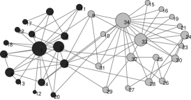
Figure 2: Zachary club network:Node color indicates community and node size indicates $u_{r,i}$. Clearly node 9,10,31 are overlapping nodes and have been identified by our algorithm.

SPAEM gives soft assignment to each node so is capable of detecting overlapping nodes, see Table 1. To compare the ability in detecting overlapping nodes, we also include $q_{ir}$ used to assign communities in the mixture model Newman and Leicht (2007). Clearly, nodes 1,2,33,34 are not overlapping nodes, but node 9 is. The mixture model also can detect this, however, by checking corresponding probabilities, see Table 1, SPAEM shows more accuracy revealing the extent of overlapping.

Table 1: Result on zachary network. $u_{r,i}$ is calculated by $u_{r,i}=\pi_{r}*\beta_{r,i}$, which is interpreted as the preference of node $i$ belonging to community $r$. The $q_{ir}$s in the mixture mode Newman and Leicht (2007) are also included, to facilitate comparison, we normalize $u_{s,i}$ so they add up to 1.

Node ID	$u_{1,i}$	$u_{2,i}$	$\frac{u_{1,i}}{u_{1,i}+u_{2,i}}$	$q_{i1}$
1	3.30E-05	0.1025	0.00	0.00
2	4.86E-06	0.0577	0.00	0.00
9	0.0219	0.0101	0.69	0.96
13	5.83E-36	0.0128	0.00	0.00
31	0.0179	0.0078	0.70	0.92
33	0.0769	1.55E-08	1.00	1.00
34	0.1090	8.20E-06	1.00	1.00

III.2 American College Football Team Network

The second network investigated is the college football network which represents the game schedule of the 2000 season of Division I of the US college football league Girvan and Newman (2002). The nodes in the network represent the 115 teams, while the links represent 613 games played. The teams are divided into 12 conferences and generally games are more frequent between members of the same conference than between teams of different conferences.

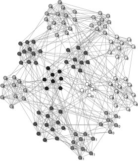
Figure 3: Result of SPAEM for American football network: Node label indicates real community membership. Nodes belonging to the same community detected by SPAEM are placed adjacently.

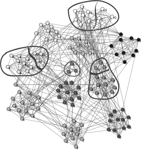
Figure 4: Result of the mixture model Newman and Leicht (2007) for American football network: Node label indicates real community membership. Nodes belonging to the same group detected are placed together, groups which are not the common sense community structure are marked using cycled line. Some of these groups are formed by nodes from two real communities. Also there is a 3 node group which is clearly not a community.

The result of SPAEM and the mixture model Newman and Leicht (2007) is depicted in FIG 3 and FIG 4, respectively. SPAEM basically uncovers the original community structure. However, the mixture model gets a very different result, see FIG 4. This is because the group it detected is a set of nodes with similar linkage property so may not be common sense community. The 3 node group in the middle of FIG 4 is obviously not a community. There are still other groups consisting of nodes from different communities, see FIG 4. The mixture model can detect patterns but it can not differentiate different kinds of patterns, in other words, it can not tell whether a detected group is a community.

III.3 Comparison With Other Methods

A modularity measure $Q=\sum_{r=1}^{c}(\frac{l_{rr}}{l}-(\frac{d_{r}}{2l})^{2})$ is proposed by Newman Newman and Girvan (2004), where $l_{rr}$ is the number of links in community $r$, $d_{r}$ is the total degree in community $r$, $l$ is the total number of edges in the network . Good community structure usually indicates large value of $Q$. But there is a scale $l$ in the definition of $Q$ and this may cause problem in some networks Fortunato and Barth lemy (2007); Rosvall and Bergstrom (2007). Such networks include those whose communities vary in size and degree sequence.

Dolphin social network reported by Lusseau Lusseau et al. (2003) provides a natural example where communities vary in size. In this network, two dolphins have a link with each other if they are observed together more often than expected by chance. The original two communities have different sizes, with one containing 22 dolphins and the other 40. Setting $c=2$, SPAEM only misclassifies one node and gets exactly the same result as the GN algorithm Girvan and Newman (2002) and the information based algorithm Rosvall and Bergstrom (2007), however, the modularity based method White and Smyth (2005) gets different result, as depicted in FIG 5.

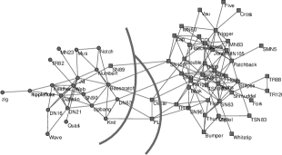
Figure 5: Dolphin network: Node shape denotes the real split. The grey line shows the result by SPAEM with only 1 mistake, the left and right black line indicates the results of algorithms in White and Smyth (2005).

It is shown that the modularity algorithm works well for networks whose communities roughly have the same size and degree sequence, but may not provide very competitive results when the communities differ in size and degree sequence Rosvall and Bergstrom (2007). To show the way SPAEM handles these situations, we conduct the same 3 sets of test as done in Rosvall and Bergstrom (2007): symmetric, node asymmetric, link asymmetric. In the symmetric test, each network is composed of 4 communities with 32 nodes each, each node has an average degree of 16, $k_{out}$ is the average number of edges linking to nodes in different communities. In the node asymmetric test, each network is composed of 2 communities with 96 and 32 nodes respectively, $k_{out}$ has the same meaning as in the symmetric test. $k_{out}$ is set to 6,7,8 in both the symmetric and node asymmetric case, as $k_{out}$ increases, it becomes difficult to detect real community structure. In the link asymmetric test, 2 communities each with 64 nodes differ in their average degree sequence, nodes in one community have average 24 edges and in the other community have only 8 edges, setting $k_{out}=2,3,4$. Table 2 gives the results of our algorithm compared to other algorithms Rosvall and Bergstrom (2007); Newman and Girvan (2004); Newman and Leicht (2007). Note that the results of the information algorithm and the modularity algorithm are cited from Rosvall and Bergstrom (2007) while results of the mixture model are calculated by the authors. We have to admit that the information algorithm outperforms all other 3 algorithms, especially in the node asymmetric and link asymmetric tests. SPAEM outperforms the modularity algorithm Newman and Girvan (2004) in the symmetric and node asymmetric tests. The mixture model Newman and Leicht (2007) seems to perform not so well in the symmetric test, this might be due to that the groups it discovers may not be communities due to fuzzy structure of these networks as $k_{out}$ increases.

Table 2: Results on the benchmark test on 3 experiment: symmetric, node asymmetric, link asymmetric.

Test	$k_{out}$	SPAEM	Compression	Modularity	Mixture
Symmetric	6	0.99	0.99	0.99	0.92
	7	0.95	0.97	0.97	0.81
	8	0.84	0.87	0.89	0.64
Node	6	0.97	0.99	0.85	0.97
Asymmetric	7	0.92	0.96	0.80	0.92
	8	0.79	0.82	0.74	0.74
Link	2	0.98	1.00	1.00	0.99
Asymmetric	3	0.94	1.00	0.96	0.94
	4	0.84	1.00	0.74	0.70

III.4 Handling Weighted Network

SPAEM can also be extended to handle weighted networks. Suppose the weighted adjacent matrix of the network is $W_{n\times n}$ with its entries $w_{i,j},i=1,2,...,n,j=1,2,...,n$, then the loglikelihood of the network becomes

$$LL=\sum_{i=1}^{n}\sum_{j:j\in N(i)}w_{i,j}\log(\sum_{r}\pi_{r}\beta_{r,i}\beta_{r,j})$$ (10)

$\overrightarrow{LL}$ becomes

$$\overrightarrow{LL}=\sum_{i=1}^{n}\sum_{j:j\in N(i)}\sum_{r}w_{i,j}q_{ij,r}\ln Pr(e_{i,j}\in r)$$ (11)

$$=\sum_{i=1}^{n}\sum_{j:j\in N(i)}\sum_{r}w_{i,j}q_{ij,r}\ln(\pi_{r}\beta_{r,i}\beta_{r,j})$$

The E-step is unchanged but M-step becomes

$$\pi_{r} =\frac{\sum_{i}\sum_{j:j\in N(i)}w_{i,j}q_{ij,r}}{\sum_{i}\sum_{j:j\in N(i)}\sum_{s}w_{i,j}q_{ij,s}}$$

$$\beta_{r,i} =\frac{\sum_{j:j\in N(i)}w_{i,j}q_{ij,r}}{\sum_{k=1}^{N}\sum_{j:j\in N(k)}w_{k,j}q_{kj,r}}$$

Intuitively the M-step formula is reasonable since links with greater weights contribute more to corresponding parameters.

To test SPAEM on weighted networks, simulation test is done as that in Alves (2007). This set of test is based on the above symmetric test when $k_{out}=8$: For each of the 100 networks in the Symmetric Test with $k_{out}=8$, the weight of edges within a certain community is raised to $w=1.4,1.6,1.8,2$, while the weight of edges running between communities is unchanged(with weight 1). As weight $w$ increases from 1.4 to 2, models should improve their power in detecting community structure. Results of SPAEM are shown in Table 3 as well as the results in Alves (2007) for comparison(note that the results in Alves (2007) are directly cited rather than recalculated). SPAEM generally outperforms the model in Alves (2007).

Table 3: Benchmark test on weighted network designed by Alves (2007). There are 4 communities each with 32 nodes in the network with $k_{out}=8$. As $w$ increase from 1.4 to 2, both methods respond positively but SPAEM gets better results.

	SPAEM	Markov
$w=1.4$	0.96	0.89
$w=1.6$	0.98	0.94
$w=1.8$	0.99	0.97
$w=2$	0.99	0.98

The limitation with the above simulation test is that any algorithm will respond positively when $w$ increases and that the original unweighted networks already have clear community structure. Now we devise a more elaborate example: consider a network with 32 nodes, each node pair has an edge with probability $p_{rand}$, obviously, this network has no community structure. Let node 1 to 16 be in group 1, node 17 to 32 be in group 2. Weight of edges inside each group is raised to 1.5 with probability $p_{weight}$ but weight of edges running between groups is unchanged. Now the only thing that can differentiate these two groups is the weight of edges. By setting $p_{rand}=0.8$ and $p_{weight}=0.8$, SPAEM uncovers the two groups with only 3 mistakes, see FIG 6. This shows SPAEM is able to take good use of edge weight.

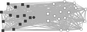
Figure 6: Results on the simulated weighted network. Node shape shows the original community while node color indicates the community structure detected by SPAEM.

III.5 Model Selection Test

Now, the minimum description length $H$ defined in Eq(II.2) is employed for SPAEM to select $c$, the optimal number of communities, and the precision is empirically set to $1/3n$. The criterion indicates that 11 communities in the American football networkGirvan and Newman (2002) should be detected, see FIG 7.a, the result seems to be wrong since there should be 12 communities, however, there is a conference “Independents” which can not be a really conference because teams in it play games with adjacent conferences. This criterion also determines 4 communities in the journal citation network, see FIG 7.b. These two results shows $H$ in Eq(II.2) and precision $1/3n$ are sound.

To further test the validity of the model selection principle , model selection results on the above simulation experiments (Symmetric, Node Asymmetric, Link Asymmetric) are presented in Table 4. Combined with the model selection principle, SPAEM gives very competitive results in all these three tests. One weird thing is that in the node asymmetric case, the accuracy of SPAEM increases as $k_{out}$ increases, this is partly because that the penalty term for describing the model parameters in Eq.(II.2) favors small number communities, this also in turn verifies that selection criterion and the precision is reasonable.

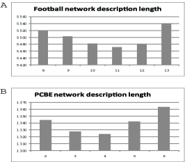
Figure 7: (a): Model selection result for American football team network. (b): Model selection result for the the journal citation network.

Table 4: Model selection result: Each entry is the fraction of networks identified with the correct number of communities, the number in the parentheses indicates the average number of communities identified by the corresponding algorithm.

Test	$k_{out}$	SPAEM-MDL	Information	Modularity
Symmetric	6	1.00(4.00)	1.00(4.00)	1.00(4.00)
	7	1.00(4.00)	1.00(4.00)	1.00(4.00)
	8	0.65(3.60)	0.14(1.93)	0.70(4.33)
Node	6	0.82(2.18)	1.00(2.00)	0.00(4.95)
Asymmetric	7	0.83(2.17)	0.80(1.80)	0.00(4.97)
	8	0.93(2.07)	0.06(1.06)	0.00(5.29)
Link	2	1.00(2.00)	1.00(2.00)	0.00(3.10)
Asymmetric	3	1.00(2.00)	1.00(2.00)	0.00(4.48)
	4	1.00(2.00)	1.00(2.00)	0.00(5.55)

III.6 Model Selection Discussion

The model selection criterion in Eq(II.2) is sensitive to the choice of the accuracy $\epsilon$, different $\epsilon$ would lead to different model selection results. Intuitively, small $\epsilon$ will favor smaller number of communities and large $\epsilon$ tends to identify large number of communities. In fact, it’s shown that complex networks may be organized in the hierarchical structure which allows us to view them in different resolutions Ravasz et al. (2002). The accuracy $\epsilon$ indeed provides the capacity to detect communities in different resolutions.

However, it is expected that for networks with well-defined community structure, the model selection criterion should be robust to the choice of accuracy $\epsilon$. To verify this, different accuracy $\epsilon$ ranging from $1/n$ to $1/7n$ are tested on the journal citation network Rosvall and Bergstrom (2007), this criterion identifies 4 communities for $\epsilon$ ranging from $1/n$ to $1/6n$ and 3 communities when $1/7n$, strongly indicating that this network actually has 4 communities. We further test how different $\epsilon$ will impact on the model selection result using the Symmetric Test when $k_{out}=6,7,8$, respectively. For $\epsilon$ ranging from $1/2n$ to $1/7n$, this criterion nearly always identifies the correct number of communities when $k_{out}=6,7$, however, when $k_{out}=8$, the accuracy drops drastically, this is due to the fuzzy structure when there are too many edges linking to other communities. The above results shows that the model selection criterion for SPAEM indeed is robust to choice of $\epsilon$ for well clustered networks.

IV CONCLUSION

In this paper, we propose a probabilistic algorithm SPAEM to resolve community structure. We have showed the power of SPAEM in detecting community structure as well as providing more useful information. SPAEM is also extended to handle weighted network. To determine the optimal number of communities, minimum description length principle is employed and tested on a variety of networks.

The mixture model in Newman and Leicht (2007) is a good algorithm capable of detecting patterns and handling directed networks while SPAEM focuses on detecting community structure. Experimentally SPAEM does perform better in uncovering community structure and identifying overlapping nodes. Though these two algorithms seem to be similar with each other, they are based on different model assumptions. Table 5 gives a summary on features of the two algorithms.

Table 5: Summary table: features of SPAEM and the Mixture model Newman and Leicht (2007)

	SPAEM	Mixture
Time Cost	$O(cl)$	$O(cl)$
Model Selection?	Yes	No
Weighted Graph?	Yes	No
Directed Graph?	No	Yes
Detect Pattern?	No	Yes

V ACKNOWLEDGMENT

This paper is supported by Science Fund for Creative Research Group, Chinese Academy of Science, No 10531070. The authors thank Dr. Martin Rosvall in Washington University and Dr. Lingyun Wu and Shihua Zhang in Chinese Academy of Science for their insightful comments on this paper. We specially thank the two anonymous reviewers for their review comments which help us to further explore the feature of our algorithm.

References

- Freeman (1992) L. C. Freeman, American Journal of Sociology 98, 152 (1992).
- LH et al. (1999) H. LH, H. JJ, L. S, and M. AW., Nature 402, 6761 (1999).
- Lusseau et al. (2003) D. Lusseau, K. Schneider, O. J. Boisseau, P. Haase, E. Slooten, and S. M. Dawson, Behavioral Ecology and Sociobiology 54, 396 (2003).
- Zachary (1977) W. W. Zachary, Journal of Anthropological Research 33, 452 (1977).
- Watts (1998) D. S. Watts, Nature 4, 409 (1998).
- A-L and R (1999) B. A-L and A. R, Science 286, 509 (1999).
- Girvan and Newman (2002) M. Girvan and M. E. J. Newman, Proc. Natl. Acad. Sci. USA 99, 7821 (2002).
- Luo et al. (2007) F. Luo, Y. Yang, C.-F. Chen, R. Chang, J. Zhou, and R. H. Scheuermann, Bioinformatics 23, 207 (2007).
- Zhou (2003) H. Zhou, Phys. Rev. E 67, 041908 (2003).
- Radicchi et al. (2004) F. Radicchi, C. Castellano, F. Cecconi, V. Loreto, and D. Parisi, Proc. Natl. Acad. Sci. USA 101, 2658 (2004).
- Zhang et al. (2007a) S. Zhang, X. Ning, and X. Zhang, Eur. Phys. J. B 57, 67 (2007a).
- Newman and Girvan (2004) M. E. J. Newman and M. Girvan, Phys. Rev. E 69, 026113 (2004).
- Newman (2006a) M. E. J. Newman, Proc. Natl. Acad. Sci. USA 103, 8577 (2006a).
- Newman (2006b) M. E. J. Newman, Phys. Rev. E 74, 036104 (2006b).
- White and Smyth (2005) S. White and P. Smyth, in SIAM International Conference on Data Mining 2005 (2005).
- Duch and Arenas (2005) J. Duch and A. Arenas, Phys. Rev. E 72, 027104 (2005).
- Fortunato and Barth lemy (2007) S. Fortunato and M. Barth lemy, Proc. Natl. Acad. Sci. USA 104, 36 (2007).
- Rosvall and Bergstrom (2007) M. Rosvall and C. T. Bergstrom, Proc. Natl. Acad. Sci. USA 104, 7327 (2007).
- Palla et al. (2005) G. Palla, I. Der nyi, I. Farkas, and T. Vicsek, Nature 435, 814 (2005).
- Zhang et al. (2006) S. Zhang, R. Wang, and X. Zhang, Physica A: Statistical Mechanics and its Applications 374, 483 (2006).
- Zhang et al. (2007b) S. Zhang, R. Wang, and X. Zhang, Phys. Rev. E 76, 046103 (2007b).
- Newman and Leicht (2007) M. E. J. Newman and E. A. Leicht, Proc. Natl. Acad. Sci. USA 104, 9564 (2007).
- Hofmann (2001) T. Hofmann, Mach. Learn. 42, 177 (2001), ISSN 0885-6125.
- Dempster et al. (1977) A. Dempster, N. Laird, and D. Rubin, Journal of the Royal Statistical Society, Series B 39, 1 (1977).
- Rissanen (1978) J. Rissanen, Automatica 14, 465 (1978).
- Ravasz et al. (2002) E. Ravasz, A. L. Somera, D. A. Mongru, Z. N. Oltvai, and A. L. Barabasi, Science 297, 1551 (2002).
- Alves (2007) N. A. Alves, Phys. Rev. E 76, 036101 (2007).