Kaon Weak Matrix Elements in 2+1 flavor DWF QCD

Abstract:

$K\to\pi$ and $K\to 0$ weak matrix elements of $\Delta S=1$ operators have been measured in 2+1 flavor domain wall fermion (DWF) QCD on (3 fm)³ lattices with $a^{-1}=1.73(3)$ GeV. As is well known, using these matrix elements and chiral perturbation theory allows a determination of the $K\to\pi\pi$ matrix elements that enter in the quantitative value for the $\Delta I=1/2$ rule and $\epsilon^{\prime}/\epsilon$. Two light dynamical sea quark masses have been used, along with six valence quark masses, with the lightest valence quark mass $\approx 1/10$ the physical strange quark mass. We report our results for lattice matrix elements in the $SU(3)_{L}\times SU(3)_{R}$ (27,1), (8,1), and (8,8) representations, paying particular attention to the statistical errors achieved after measurements on 75 configurations. We also report on our calculation of the non-perturbative renormalization coefficients for these $\Delta S=1$ weak operators, using the Rome-Southampton method.

1 Introduction

CP violation is now a well established property of Nature, having been observed in both kaon and B meson systems. Its standard model explanation, that the violation arises from the difference between the mass and weak interaction eigenstates of the quarks, is quantitatively encapsulated in the unitary $3\times 3$ Cabbibo-Kobayashi-Maskawa (CKM) matrix which relates these eigenstates. Determining the elements of this matrix is the subject of extensive theoretical and experimental effort. However, even assuming precise values for the elements of the CKM matrix, a prediction for the rate of direct CP-violating decays in kaons, determined experimentally by measuring the quantity Re($\epsilon^{\prime}/\epsilon$), is lacking. Such a prediction relies on values for the hadronic $K\to\pi\pi$ matrix elements of low-energy, four-quark operators. Lattice QCD is the only first principles method to allow determination of these matrix elements and their measurement has been the subject of many studies. In this note, we discuss our progress in determining these matrix elements, using full 2+1 flavor QCD with domain wall quarks.

Euclidean space lattice methods for the direct evaluation of the desired $K\to\pi\pi$ matrix elements have been developed, and some preliminary studies have been performed [1, 2]. However, to reach physical values for the kaon and pion masses in full QCD simulations is beyond the reach of current computers. Here we follow the long-standing approach of using chiral perturbation theory to relate $K\to\pi\pi$ matrix elements to matrix elements of the same operator measured in $K\to\pi$ and $K\to 0$ matrix elements [3]. Quenched calculations have been done with this approach [4, 5], which showed that with DWF, the problems of lower dimensional operator mixing at finite lattice spacing and renormalization of the operators were under good control. Statistically well resolved values for the lowest order chiral perturbation theory constants were achieved and, by naively extending lowest order chiral perturbation theory to the kaon mass, physical results were quoted.

However, for these particular kaon weak matrix elements calculations, it was pointed out that quenching makes the relation between the full QCD chiral perturbation theory constants and the quenched ones ambiguous [6, 7, 8], providing a source of uncertainty in interpreting the quenched calculation that is more serious than the general caution that must be exercised with quenching. In the current 2+1 flavor calculation, these ambiguities are removed.

To date, our calculation involves measuring the same operators as in our previous quenched calculation [4], although on larger volume lattices, with 2+1 dynamical flavors and with much lighter valence quark masses [9, 10]. With these valence masses, we see that next-to-leading order (NLO) SU(3) chiral perturbation theory for pseudoscalar decay constants and masses [11], and the pseudoscalar bag parameter $B_{PS}$ (the analogue of $B_{K}$ with two light quarks in the “kaon”) [12], represents the lattice data at the $\approx 5$% level or better. Thus we can try similar NLO chiral perturbation theory fits to the data presented here, which covers a similar range of pseudoscalar masses, in the hopes of extracting the desired low energy constants. These fits require the 2+1 flavor partially quenched chiral perturbation theory formula for our matrix elements, a calculation which is underway [13].

We also discuss the status of our calculation of the non-perturbative renormalization Z factors needed to convert our lattice results to $\overline{\rm MS}$ conventions.

2 Simulation Details

We have measured the 10 $\Delta S=1$ operators needed for a determination of $\epsilon^{\prime}/\epsilon$ and the $\Delta I=1/2$ rule, using the notation of [4]. When evaluated between $K^{+}$ and $\pi^{+}$ states, the operators produce the contractions shown in Figure 1. The contractions between kaons and pions are known as figure eight diagrams and eye diagrams. We also need vacuum diagrams and contractions involving $\bar{s}d$, to remove the mixing with lower dimensional operators. We use Coulomb gauge fixed wall sources at $t=5$ and 59 on our $24^{3}\times 64\times 16$ lattices as the sources for the kaons and pions. The Dirac equation is solved twice for each wall source, once with periodic and once with anti-periodic boundary conditions, and the two solutions added to effectively double the length of the lattice in the time direction. Our operator contractions are always done with $5\leq t_{op}\leq 59$, where $t_{op}$ is the time where the operator is evaluated, so the double lattice merely serves to suppress any contributions to our operators from propagation around the world in the time direction.

For the closed fermion loops in the eye and $K\to 0$ contractions, we use a stochastic source, spread over the spatial volume and covering all time slices from 12 to 51 (40 time slices). A single stochastic source is a fixed spin and color component, with a space-time value that is Gaussianly distributed. For each spin and color combination, solutions are found for four different stochastic space-time distributions.

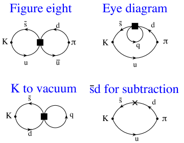
Figure 1: The contractions used in the evaluation of the $\Delta S=1$ operators that have been calculated in this report. The sources for the kaons and pions are Coulomb gauge fixed wall sources and the closed fermion loop contractions are calculated with stochastic sources.

For each configuration, 6 valence quark masses are used: $m_{f}=0.001$, 0.005, 0.01, 0.02, 0.03, 0.04. The residual quark mass from the finite $L_{s}$ extent of our lattices is 0.00315(2) [11]. These bare quark masses correspond to pseudoscalar masses ranging from 250 MeV to 750 MeV. From fits to pseudoscalar masses and decay constants, we find that for the three lightest bare quark masses (0.001, 0.005 and 0.01), NLO chiral perturbation theory agrees well with our measured data.

For each configuration, we do 8 full (all spins and colors for the source) five-dimensional solutions to the Dirac equations for each valence mass. Each wall source requires 2 solutions (one for each boundary condition) and we do four stochastic estimators for the closed fermion loops. Thus we spend half of the time on the wall source inversions and half on the stochastic inversions.

The results reported here are for 76 configurations, separated by 40 molecular dynamics time units, for our ensemble with light dynamical quark mass $m_{l}=0.005$ and 74 configurations, with the same separation, for $m_{l}=0.01$. To do these 8 full inversions for the six valence quark masses on a single configuration takes about 24 hours on a 4,096 node QCDOC partition, with the lightest valence quark mass taking about half of the total time.

3 Chiral Perturbation Theory and Ward Identity Test

In the 3 flavor effective theory that comes from integrating out the charm, bottom and top quarks (as well as the weak vector bosons), the effective Hamiltonian for $\Delta S=1$ transitions is

$${\cal H}^{(\Delta S=1)}=\frac{G_{F}}{\sqrt{2}}V_{ud}V_{us}^{*}\left\{\sum_{i=1}^{10}\left[z_{i}(\mu)+\tau y_{i}(\mu)\right]Q_{i}\right\}$$ (1)

Here $z_{i}(\mu)$ and $y_{i}(\mu)$ are Wilson coefficients and the $Q_{i}$ are four-quark operators. Of the ten four-quark operators $Q_{i}$ above, only seven are independent, and they include three representations of $SU(3)_{L}\times SU(3)_{R}$: (27,1), (8,1) and (8,8). In lowest order chiral perturbation theory, the desired $K\to\pi\pi$ matrix elements are all proportional to an appropriate low energy constant, denoted as $\alpha_{1}^{(8,1)}$, $\alpha^{(27,1)}$, or $\alpha^{(8,8)}$. These come from $K\to\pi$ and $K\to 0$ matrix elements as given in Table 1. Note that for the (8,1) operators, to determine the physically relevant quantity $\alpha_{1}^{(8,1)}$ requires remove the power divergent quantity $\alpha_{2}^{(8,1)}$, which is measured in $K\to 0$ matrix elements

Irrep	Number	Isospin	$K^{+}\to\pi^{+}$	$K^{0}\to\pi^{+}\pi^{-}$
(27,1)	1	1/2, 3/2	$-\frac{4m_{M}^{2}}{f^{2}}{\alpha^{(27,1)}}$	$-\frac{4i}{f^{3}}m_{K^{0}}^{2}{\alpha^{(27,1)}}$
(8,1)	4	1/2	$\frac{4m_{M}^{2}}{f^{2}}({\alpha^{(8,1)}_{1}}-{\alpha^{(8,1)}_{2}})$	$\frac{4i}{f^{3}}m_{K^{0}}^{2}{\alpha^{(8,1)}_{1}}$
(8,8)	2	1/2, 3/2	$-\frac{12}{f^{2}}{\alpha^{(8,8)}}$	$-\frac{12i}{f^{3}}{\alpha^{(8,8)}}$

Table 1: The relation between matrix elements and low energy constants, to lowest order in chiral perturbation theory. The second column gives the number of different operators transforming as the given irreducible representation.

To accurately determine the leading order chiral perturbation theory constants, we want to try to fit our matrix element data to the full partially quenched 2+1 flavor formulae. Calculations of these formulae are underway [13], and when they are complete, we will fit our data to them in our efforts to extract the best values for the $\alpha$’s.

Since NLO chiral perturbation theory plays such an important role here, we turn briefly to a simple matrix element $\langle\pi^{+}|\bar{s}d|K^{+}\rangle$ that is known in chiral perturbation theory and that also enters our calculation. At leading order in chiral perturbation theory, one has

$$\frac{2m_{f}}{m_{\pi}^{2}}\langle\pi^{+}|\bar{s}d|K^{+}\rangle-1=0$$ (2)

We calculate this from the ratio of a three point function to two, 2-point functions as

$$R_{2}\equiv\frac{\langle P_{\pi^{+}}^{\rm wall}(x_{0})\,[\bar{s}d](y)\,P_{K^{-}}^{\rm wall}(z_{0})\rangle}{\langle P_{\pi^{+}}^{\rm wall}(x_{0})\,P_{\pi^{-}}^{\rm wall}(z_{0})\rangle}$$ (3)

Here $P^{\rm wall}_{\pi^{+}}$ is a wall Coulomb gauge fixed pseudoscalar wall source with the quantum numbers of the $\pi^{+}$. $R_{2}$ differs from $\langle\pi^{+}|\bar{s}d|K^{+}\rangle$ by known factors.

Figure 2 shows a plot of the appropriately scaled $R_{2}$ versus valence input quark mass for the current 2+1 flavor full QCD ensembles and the same results for our earlier quenched ensemble. In the limit $m_{f}\to-m_{\rm res}$ and the light sea and valence quarks are equal, the curves should go to 1. We can see that there is noticeable curvature in the graphs for quark masses below 0.01 and there is a small dynamical quark mass effect when comparing the $m_{l}=0.005$ and 0.01 ensembles. This is certainly the region where partially quenched chiral logarithms should be noticeable, and are seen in our other observables, but fits to the precise formulae (when available) will be required to sharpen this general statement. For $B_{PS}$ [12] we do see that the partially quenched logarithms have a curvature that is opposite the curvature when the valence and sea quark masses are the same. Also note that the curvature is much more noticeable in the dynamical ensemble data than the quenched results and that the valence masses in the current work are much lighter than the earlier quenched work.

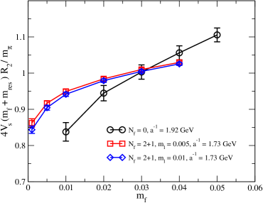
Figure 2: A plot of the appropriately scaled $\langle\pi^{+}|\bar{s}d|K^{+}\rangle$ versus valence quark mass. When the valence and sea quark masses are equal, the curves should go to 1.

4 $\Delta I=3/2$ Matrix Elements

We now turn to the $\Delta I=3/2$ matrix elements and present some of our lattice data. The 3/2 part of $Q_{2}$ and $Q_{8}$ are presented in Figure 3. We see at once that we have very long plateaus which extend, with essentially uniform errors, across the lattice. We choose to fit the plateau from $t=12$ to 51, i.e. starting from a distance of 7 away from the two wall sources. Clearly with such long plateaus the results are not sensitive to the precise fit range chosen. The average value, with error bars, for each mass is indicated by the horizontal lines on the graphs.

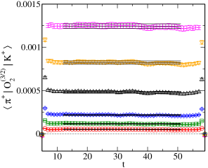
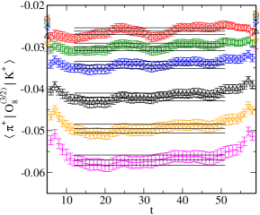
Figure 3: Plateaus for the $\Delta I=3/2$ part of the $K\to\pi$ matrix elements of $Q_{2}$ and $Q_{8}$. For $Q_{2}$ (left panel) the valence masses run from the largest (top points) to the smallest (bottom), while for $Q_{8}$ (right panel) they run from the smallest (top points) to the largest (bottom). The pseudoscalars have degenerate quark masses.

In Figure 4, we present values for $Q_{2}^{(3,2)}$ as a function of valence quark mass for our previous quenched calculation (left panel) and the $m_{l}=0.005$ lattices from our current ensemble. Note the much smaller range of quark masses plotted in the 2+1 flavor QCD case. In our earlier quenched work, we saw no strong indication of quenched chiral logarithms, but found a large contribution from the analytic NLO terms. We do not yet have the chiral perturbation theory formulae for the 2+1 flavor case, nor the fits to the data. However, one can see that some downward curvature is needed to have the extrapolated matrix element vanish at the origin, as required by chiral symmetry. Also, for these much smaller valence quark masses, one does not readily see a noticeable effect of higher order analytic terms.

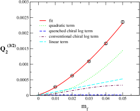
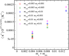
Figure 4: A comparison of the lattice normalized matrix elements for our earlier quenched calculation (left panel) and the current 2+1 flavor calculation (right panel).

5 Weak Matrix Elements in the (8,1) Representation

5.1 (8,1) Operators

Among the 10 weak operators involved in the $K\to\pi\pi$ process below the charm threshold, $Q_{i}\,\left\{i=3,4,5,6\right\}$ are pure (8,1) $\Delta I=1/2$ operators, while $Q_{i}\,\left\{i=1,2,9,10\right\}$ have both (8,1), $\Delta I=1/2$ and (27,1), $\Delta I=1/2$ parts. The (8,1) operators are particularly important for the investigation of CP violation, since, from the size of the Wilson coefficients at 2 GeV, the matrix element of $Q_{6}$ is dominant in $\mathrm{Im}\left(A_{0}\right)$ [4].

Since the $\Delta I=1/2$ operators can mix with the quadratically divergent operator $\Theta^{\left(3,\bar{3}\right)}\equiv\bar{s}\left(1-\gamma_{5}\right)d$, their $K\to\pi$ matrix elements alone cannot determine the relevant $K\to\pi\pi$ elements. It is necessary to evaluate their $K\to 0$ matrix elements to remove the unwanted contributions.

5.2 Plateaus of $K\to\pi$ for (8,1) Operators

As mentioned earlier, we evaluate the value of $\left\langle\pi^{+}\left|Q_{i}\right|K^{+}\right\rangle$, by placing Coulomb gauge fixed wall sources at $t_{K}=5$ and $t_{\pi}=59$. The eye contractions that appear in (8,1) operators are determined with random sources with support from $t_{rand}=12$ to 51. We can then evaluate the operator contribution from any timeslice given by $t_{op}$ with $12\leq t_{op}\leq 51$. By taking the ratios of the three- and two-point pseudoscalar-pseudoscalar Green’s functions we calculate the required matrix elements [4]. As an example, Figure 5 shows the plateaus for $\left\langle\pi^{+}\left|Q_{6}\right|K^{+}\right\rangle$. With either degenerate or non-degenerate valence masses, we have very long plateaus (40 time-slices). Comparing these graphs with the plateaus in Figure 3, we see that the error bars here, after averaging over time slices (black horizontal lines) are smaller than the error bars for the individual points. Such an effect is not very noticeable in the $\Delta I=3/2$ amplitudes of Figure 3.

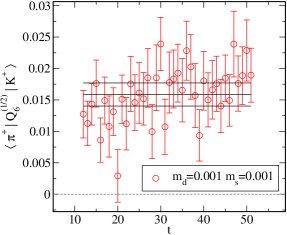
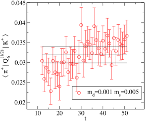
Figure 5: Plateaus of $\left\langle\pi^{+}\left|Q_{6}\right|K^{+}\right\rangle$ with $m_{\mathrm{sea}}=0.005$. Figure (a) has degenerate valence masses ($m_{d}=m_{s}=0.001$) and Figure b) has non-degenerate valence quark ($m_{d}=0.001$, $m_{s}=0.005$). In both cases, the matrix elements have long plateaus.

5.3 Resolving Quadratic Divergence with $K\to 0$ Matrix Elements

As explained earlier, we need to calculate the $K\to 0$ matrix elements for $\Delta I=1/2$ operators to remove the mixing with lower dimensional operators. For the (8,1) operators, we determine a mixing coefficient $\eta_{1,i}$ as in [4] by calculating

$$\frac{\left\langle 0\left|Q_{i,\mathrm{lat}}^{\left(1/2\right)}\right|K^{0}\right\rangle}{\left\langle 0\left|\left(\bar{s}\gamma_{5}d\right)_{\mathrm{lat}}\right|K^{0}\right\rangle}=\eta_{0,i}+\eta_{1,i}\left(m_{s}-m_{d}\right)$$ (4)

where the valence quark masses have $m_{s}\neq m_{d}$. Again using $Q_{6}$ as an example, Figure 6 shows the plateau of the $K\to 0$ matrix element in the left panel and the result of fitting to Eq. 4 above. One sees that the data shows a very accurate linear dependence on $m_{s}-m_{d}$, which is expected since the quadratically divergent part of $Q_{6}$ dominates the numerator and it is proportional to $m_{s}-m_{d}$. Since $Q_{6}$ has the largest divergent contribution, its matrix elements show the best linearity. For other operators, with a smaller divergent part, the linearity is less good, but also the required cancellation in the subtraction of the divergent part is less stringent.

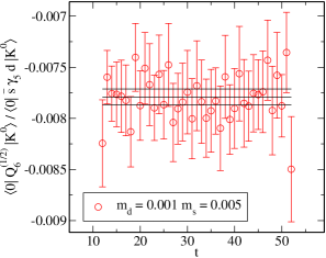
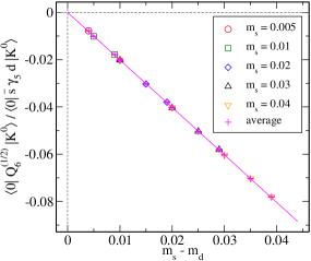
Figure 6: Calculating mixing coefficient between four-quark operators and $\bar{s}d$ using the ratio $\left\langle 0\left|Q_{i,\mathrm{lat}}^{\left(1/2\right)}\right|K^{0}\right\rangle/\left\langle 0\left|\left(\bar{s}\gamma_{5}d\right)_{\mathrm{lat}}\right|K^{0}\right\rangle$. Figure (a) shows the plateau of the matrix element with $m_{\mathrm{sea}}=0.005$, $m_{d}=0.001$, and $m_{s}=0.005$. Figure (b) shows the results of fitting to $(m_{s}-m_{d})$, which reveals a nice linear structure.

5.4 Subtraction of the Quadratic Divergence

After calculating the mixing coefficient $\eta_{1,i}$, we use it to subtract the quadratically divergent contribution of $\left\langle\pi^{+}\left|\bar{s}d\right|K^{+}\right\rangle$ from the raw matrix elements [4].

$$\left\langle\pi^{+}\left|Q_{i}^{\left(8,1\right)}\right|K^{+}\right\rangle_{\mathrm{sub}} \equiv\left\langle\pi^{+}\left|Q_{i}^{\left(8,1\right)}\right|K^{+}\right\rangle+\eta_{1,i}\left(m_{s}+m_{d}\right)\left\langle\pi^{+}\left|\bar{s}d\right|K^{+}\right\rangle$$ (5)

$$=\frac{4\alpha_{1}^{\left(8,1\right)}}{f^{2}}m_{K}m_{\pi}+\left(chiral\;logs\right)+(analytic\;terms)$$ (6)

where the second line is the prediction of the chiral perturbation theory. (The cancellation of the power divergences is true without reference to chiral perturbation theory.) While we have begun fitting to next-to-leading order 2+1 flavor partially quenched chiral perturbation theory, the formulae are still being checked, so we have also experimented with simple leading order fits.

Figure 7(a) shows the subtraction process for $Q_{6}$. Since $Q_{6}$ is the most divergent, the subtraction term (green squares) is very close to the unsubtracted matrix elements, and thus a precise determination of the subtraction term is vital. (This was also the case in the quenched calculations.) In Figure 7(b), we show the subtracted matrix elements $\left\langle\pi^{+}\left|Q_{6}\right|K^{+}\right\rangle_{\mathrm{sub}}$, including all non-degenerate combinations of valence masses $\left(m_{d},\,m_{s}\right)$, and also the result of fitting them to the leading order term in chiral perturbation theory, $m_{K}m_{\pi}$. The plots show that the data fit the leading order theory very well. Of course, here our error bars are larger than for the $\Delta I=3/2$ matrix elements and modest chiral logarithm effects are consistent with the apparent linearity of our data and our error bars. It remains an open question as to whether we can achieve statistical accuracy for the subtracted (8,1) operators that is the same size as the predicted effects of chiral logarithms.

Due to the existence of power divergences and the fact that the residual chiral symmetry breaking effects in divergent amplitudes are not strictly proportional to $m_{\rm res}$ , the subtracted matrix elements do not have to vanish at the chiral limit [4]. (Recall that the physical quantity of interest is the slope of the subtracted matrix elements.) Rather, at the chiral limit, their deviation from zero should be an $\mathcal{O}\left(m_{\mathrm{res}}\right)$ effect. In Figure 7(b), the top line does not use $m_{\mathrm{res}}$ in the subtraction process (Eq.5), while the bottom line does subtraction with $m_{\mathrm{sea}}$. As these two lines bracket the zero point at the chiral limit, the above expectation is verified.

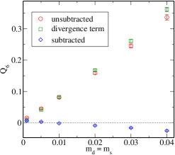
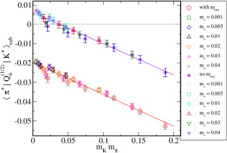
Figure 7: Subtraction of quadratic divergence from $K\to\pi$ matrix elements. Figure (a) shows the subtraction process for degenerate valence masses $m_{d}=m_{s}$. It is clear that for the divergent operator, the physical quantity is very sensitive to any noise in the matrix elements. Figure (b) fits the subtracted matrix elements $\left\langle\pi^{+}\left|Q_{6}\right|K^{+}\right\rangle_{\mathrm{sub}}$ with all available pairs of non-degenerate valence masses to the leading order term $m_{K}m_{\pi}$. The upper line does not use $m_{\mathrm{res}}$ while on the lower line each subtraction has used $m_{\mathrm{res}}$. Both figures present the data of $m_{\mathrm{sea}}=0.005$ ensemble.

5.5 PQS vs. PQN

As we work in the 2+1 flavor partially quenched theory, there are different methods to make contractions with the four-quark operators which have a singlet piece, i.e. PQS vs. PQN [8, 14, 15, 16]. The operators $Q_{i}\>\left\{i=3,4,5,6\right\}$ all have a singlet part in their operator definition,

$$Q_{i}\equiv\left(\bar{s}d\right)_{L}\sum_{q\in\left\{u,d,s\right\}}\left(\bar{q}q\right)_{L\ \mbox{or}\ R}.$$ (7)

When evaluating their weak matrix elements on our partially quenched lattices, we may either keep the singlet structure of the operator, such that the summation will become a sum over all valence, sea, and ghost quarks, or we only sum over the valence quarks as we shall do in full QCD. The former, as we keep the singlet property, is called the PQS (partially quenched singlet) method, while the latter is called the PQN (partially quenched non-singlet) method.

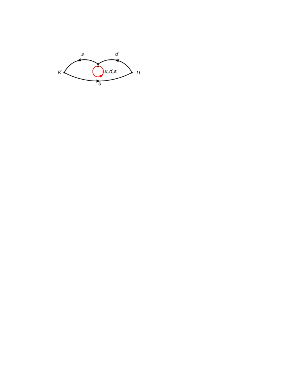
Figure 8: Quark flow diagrams needed to evaluate the weak matrix elements for $Q_{i}\>\left\{i=3,4,5,6\right\}$. A connected line represents a trace over spin indices. Only diagram (b) has differs between the PQS and PQN method. With the PQS method, the quark loop (red) will be constructed from sea quarks, while with the PQN method, it will be constructed from valence quarks.

On the quark level, calculating the weak matrix elements of the above operators requires the evaluation of the three quark-flow diagrams shown in Figure 8. The only difference between PQS and PQN is in diagram (b). With the PQS method, the summation on the quark self-contraction (the red quark loop) will go over all valence, sea, and ghost quarks (and since valence loops cancel with ghosts, only the sum over sea remains). With the PQN method, the sum will go over the valence quarks only.

We have calculated the subtracted matrix elements with both the PQS and PQN methods (Table 2). The comparison of the slope of the subtracted matrix elements (w.r.t $m_{K}m_{\pi}$), which is the leading order coefficient for (8,1) operators, shows small differences between the two methods. We see that this ambiguity does not affect the chiral fits significantly on our 2+1 flavor partially quenched lattices.

Slope of $\left\langle\pi^{+}\left|Q_{i}\right|K^{+}\right\rangle_{\mathrm{sub}}$	3	4	5	6
PQS	$0.0009(37)$	$0.0383(27)$	$-0.0626(53)$	$-0.183(13)$
PQN	$-0.0042(38)$	$0.0373(34)$	$-0.0638(55)$	$-0.165(14)$

Table 2: Comparison between the PQS and PQN methods of the slope of the subtracted $K\to\pi$ matrix elements (w.r.t $m_{K}m_{\pi}$).

6 Non-perturbative Renormalization for $\Delta S=1$ Operators

6.1 NPR Procedure

To convert the bare lattice quantities into the continuum scheme, we have employed the Rome-Southampton non-perturbative renormalization prescription [17]. Following the procedure as described in ref. [4], we write the NPR formula as

$$O_{i}^{\mathrm{cont,\,ren}}\left(\mu\right)=\sum_{j}Z_{ij}\left(\mu\right)\left[O_{j}^{\mathrm{lat}}+\sum_{k}c_{k}^{j}\left(\mu\right)B_{k}^{\mathrm{lat}}\right]+\mathcal{O}\left(a\right)$$ (8)

where $O_{i}$ are the dimension 6 operators, and $B_{k}$ are the lower dimensional operators. The NPR calculation is done on $16^{3}\times 32\times 16$ lattices [18] which have been generated with the same parameters as our $24^{3}\times 64\times 16$ lattices, except that the lightest dynamical quark mass on the smaller volume is 0.01.

To simplify the computation, we have eliminated $Q_{4}$, $Q_{9}$, and $Q_{10}$ from the 10-operator basis, since they can be written as linear combination of the other operators [4]. Further, we rotate the remaining 7-operator basis such that each operator is in a distinct $SU(3)\otimes SU(3)$ representation. The transformation relation can be found in ref.[4]. The new set of operators is denoted as $Q_{i}^{\prime}$.

6.2 Resolving the Mixing with Lower Dimensional Operators

To resolve the mixing between the four quark operator and the lower dimensional operators, we consider the two most divergent lower dimensional ones [4]:

$$B_{1} \equiv\bar{s}d$$

$$B_{2} \equiv\bar{s}\left(-\overleftarrow{\not{D}}+m_{s}\right)d+\bar{s}\left(\overrightarrow{\not{D}}+m_{d}\right)d.$$ (9)

To compute the corresponding mixing coefficients $c_{1}^{i}$ and $c_{2}^{i}$, we have used two conditions

$$\mathrm{Tr}\left[\left\langle s\left(p\right)O_{i}^{\mathrm{sub}}\bar{d}\left(p\right)\right\rangle_{\mathrm{amp}}\right] =0$$

$$\mathrm{Tr}\left[i\not{p}\left\langle s\left(p\right)O_{i}^{\mathrm{sub}}\bar{d}\left(p\right)\right\rangle_{\mathrm{amp}}\right] =0$$ (10)

with propagators evaluated at unitary masses ($m_{d}=m_{s}=m_{\mathrm{sea}}$).

6.3 Resolving the Mixing between Four-Quark Operators

To determine the mixing coefficient between the 7 operators in the new basis, we construct a set of external quark combinations $E_{\alpha\beta\gamma\delta}^{j}$ [4]. Then we impose the renormalization condition that

$$\frac{1}{Z_{q}^{2}}Z^{ki}\Gamma_{\beta\alpha\delta\gamma}^{j}\left\langle O_{i}^{\mathrm{sub}}E_{\alpha\beta\gamma\delta}^{j}\right\rangle_{\mathrm{amp}}=F^{kj}$$ (11)

where $\Gamma_{\beta\alpha\delta\gamma}^{j}$ is the projector corresponding to the spin and color structure of the operator $j$, and there is no sum over $j$ in the above equation. On the r.h.s, $F^{kj}$ is the free field limit of the matrix $\Gamma_{\beta\alpha\delta\gamma}^{j}\left\langle O_{i}^{\mathrm{sub}}E_{\alpha\beta\gamma\delta}^{j}\right\rangle_{\mathrm{amp}}$. $Z_{q}^{1/2}$ is the quark wavefunction renormalization factor [19].

The calculation of the combination $\Gamma_{\beta\alpha\delta\gamma}^{j}\left\langle O_{i}^{\mathrm{sub}}E_{\alpha\beta\gamma\delta}^{j}\right\rangle_{\mathrm{amp}}$ requires evaluation of the many quark flow diagrams that can possibly be constructed with the relevant operator and the external quark combination. Figure 9 shows 4 out of 248 quark flow diagrams involved in the evaluation of renormalization coefficient for $Q_{1}^{\prime}$. Each diagram is evaluated at unitary quark mass and non-exceptional external momenta $p_{1}$ and $p_{2}$ where $p_{1}^{2}=p_{2}^{2}=\left(p_{1}-p_{2}\right)^{2}$ [4].

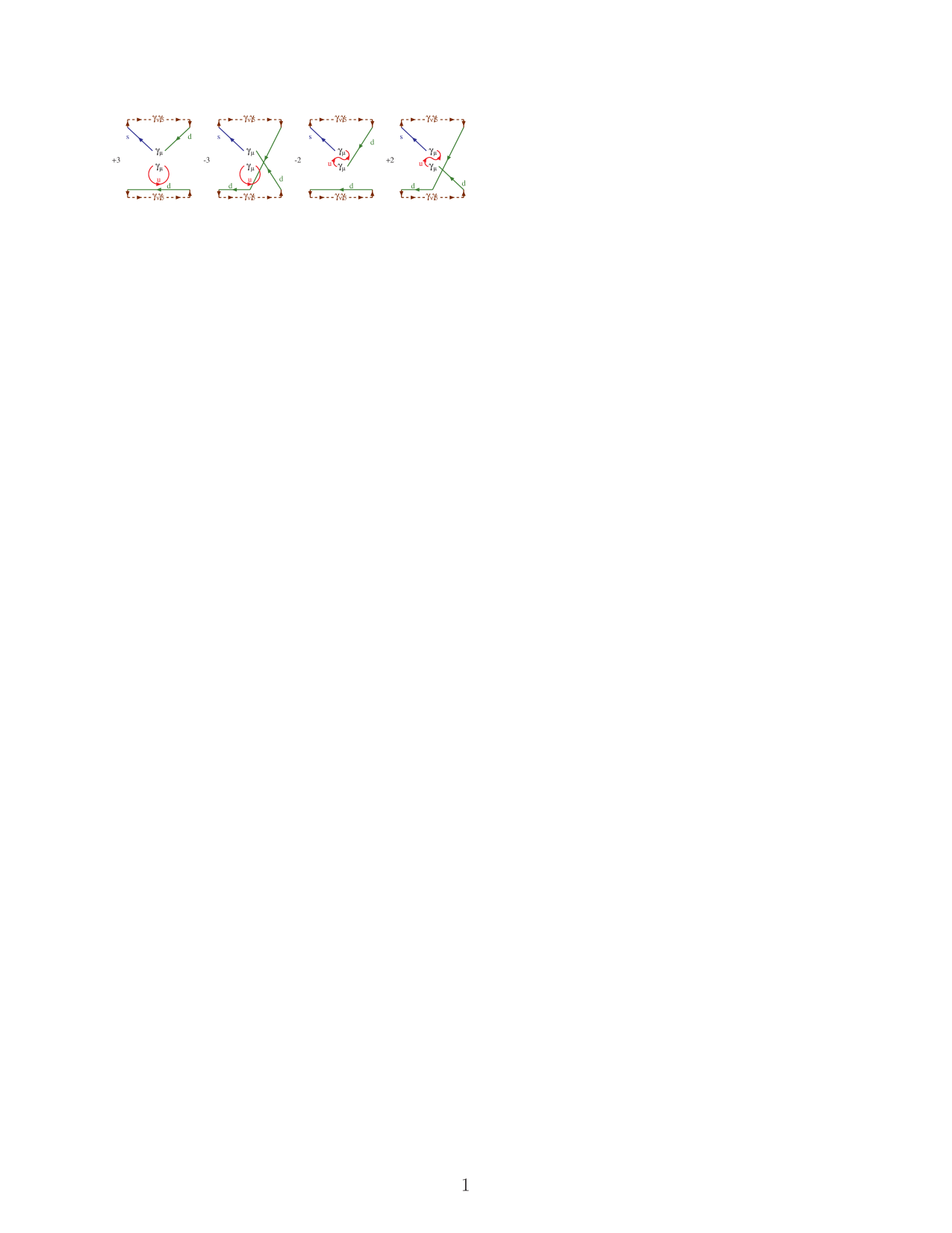
Figure 9: 4 out of 248 quark flow diagrams with their corresponding factors involved in the calculation of the mixing coefficients between $Q_{1}^{\prime}$ and $Q_{1}^{\prime}$. The solid lines represent quark propagators and each loop formed by solid and dashed lines represents a trace over spin and color indices.

After the evaluation of the entire matrix of mixing coefficients, we remove the coefficients that are both theoretically suppressed and statistically zero, and then fit the remaining matrix to a unitary mass dependence (Figure 10(a)). Since one of the lower dimensional mixing coefficients, $c_{1}^{i}$, is expected to have the mass dependence $m/a^{2}$ at leading order, this step will automatically remove $c_{1}^{i}$. Then the subtraction of the other, $c_{2}^{i}$, is performed. Due to its small magnitude, this subtraction does not make big differences in the final result (Figure 10(b)).

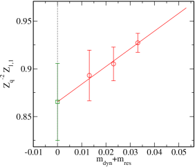
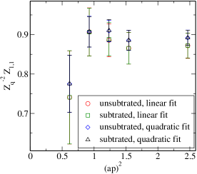
Figure 10: Evaluation of the mixing coefficients between four quark operators. Figure (a) shows the linear mass fit of the mixing coefficient $Z_{q}^{-2}Z_{1,1}$. Figure (b) shows the final value of $Z_{q}^{-2}Z_{1,1}$ at 5 different momentum scales where we have sufficient pairs of non-exceptional momenta $\left(p_{1},\,p_{2}\right)$ to evaluate the quark flow diagrams. Also in Figure (b), we show a comparison between linear and quadratic mass fits, as well as a comparison between the values before and after the subtraction of $c_{2}^{i}$. It is clear that the differences are not significant.

7 Conclusions

We have discussed the status of measurements of $K\to\pi$ and $K\to 0$ weak matrix elements on $24^{3}\times 64$, 2+1 flavor dynamical domain wall lattices by the RBC and UKQCD collaborations. We are working at much smaller masses and larger volumes than earlier quenched calculations and, with the 2+1 flavor ensembles, we are free of quenching errors. We find good statistical errors and long plateaus for our measured matrix elements and the subtraction of power divergent operator mixing contributions to (8,1) operators works as expected. We find that the ambiguity between the PQS and PQN methods is removed. The non-perturbative renormalization of our operators, following the Rome-Southampton prescription, is essentially complete. We await the completion of the NLO $PQ\chi PT$ formulae for these matrix elements, and preliminary fits are underway. The accuracy and stability of these fits will play a large role in determining our final errors.

References

- [1] L. Lellouch and M. Luscher, Commun. Math. Phys. 219, 31 (2001), hep-lat/0003023.
- [2] C. Kim UMI-31-47246.
- [3] C. W. Bernard, T. Draper, A. Soni, H. D. Politzer, and M. B. Wise, Phys. Rev. D32, 2343 (1985).
- [4] T. Blum et al. (RBC), Phys. Rev. D68, 114506 (2003), hep-lat/0110075.
- [5] J. I. Noaki et al. (CP-PACS), Phys. Rev. D68, 014501 (2003), hep-lat/0108013.
- [6] M. Golterman and E. Pallante, JHEP 10, 037 (2001), hep-lat/0108010.
- [7] M. Golterman and E. Pallante, Phys. Rev. D69, 074503 (2004), hep-lat/0212008.
- [8] M. Golterman and E. Pallante, Phys. Rev. D74, 014509 (2006), hep-lat/0602025.
- [9] D. J. Antonio et al. (RBC and UKQCD), PoS LAT2006, 188 (2006).
- [10] D. J. Antonio et al. (RBC and UKQCD) (2007), hep-ph/0702042.
- [11] M. Lin and E. E. Scholz (RBC and UKQCD), these proceedings .
- [12] D. J. Antonio and S. D. Cohen (RBC and UKQCD), these proceedings .
- [13] C. Aubin, J. Laiho, and S. Li, in preparation .
- [14] M. Golterman and E. Pallante, PoS LAT2006, 090 (2006), hep-lat/0610005.
- [15] J. Laiho and A. Soni, Phys. Rev. D71, 014021 (2005), hep-lat/0306035.
- [16] C. Aubin et al., Phys. Rev. D74, 034510 (2006), hep-lat/0603025.
- [17] G. Martinelli, C. Pittori, C. T. Sachrajda, M. Testa, and A. Vladikas, Nucl. Phys. B445, 81 (1995), hep-lat/9411010.
- [18] C. Allton et al. (RBC and UKQCD), Phys. Rev. D76, 014504 (2007), hep-lat/0701013.
- [19] T. Blum et al., Phys. Rev. D66, 014504 (2002), hep-lat/0102005.