Two-component jet simulations

Abstract

Context. Observations of collimated outflows in young stellar objects indicate that several features of the jets can be understood by adopting the picture of a two-component outflow, wherein a central stellar component around the jet axis is surrounded by an extended disk-wind. The precise contribution of each component may depend on the intrinsic physical properties of the YSO-disk system as well as its evolutionary stage.

Aims. In this context, the present article starts a systematic investigation of two-component jet models via time-dependent simulations of two prototypical and complementary analytical solutions, each closely related to the properties of stellar-outflows and disk-winds. These models describe a meridionally and a radially self-similar exact solution of the steady-state, ideal hydromagnetic equations, respectively.

Methods. By using the PLUTO code to carry out the simulations, the study focuses on the topological stability of each of the two analytical solutions, which are successfully extended to all space by removing their singularities. In addition, their behavior and robustness over several physical and numerical modifications is extensively examined. Therefore, this work serves as the starting point for the analysis of the two-component jet simulations.

Results. It is found that radially self-similar solutions (disk-winds) always reach a final steady-state while maintaining all their well-defined properties. The different ways to replace the singular part of the solution around the symmetry axis, being a first approximation towards a two-component outflow, lead to the appearance of a shock at the super-fast domain corresponding to the fast magnetosonic separatrix surface. These conclusions hold true independently of the numerical modifications and/or evolutionary constraints that the models have been undergone, such as starting with a sub-modified-fast initial solution or different types of heating/cooling assumptions. Furthermore, the final outcome of the simulations remains close enough to the initial analytical configurations showing thus, their topological stability. Conversely, the asymptotic configuration and the stability of meridionally self-similar models (stellar-winds) is related to the heating processes at the base of the wind. If the heating is modified by assuming a polytropic relation between density and pressure, a turbulent evolution is found. On the other hand, adiabatic conditions lead to the replacement of the outflow by an almost static atmosphere.

1 Introduction

Observations made over the last two decades have shown that one class of the widespread astrophysical phenomenon of collimated plasma outflows (jets) is being launched from the vicinity of most young stellar objects (YSOs) (Burrows et al. Bur96 (1996)). These supersonic mass outflows are found to be correlated with accretion (Cabrit et al. Cab90 (1990); Hartigan et al. Har95 (1995)), to have narrow opening angles (Ray et al. Ray96 (1996)) and to propagate for several orders of magnitude of spatial distances ranging from the AU to the pc scales (Dougados et al. Dou00 (2000); Hartigan et al. Har04 (2004)). A central role in the launching, acceleration and collimation of these jets is widely believed to be played by magnetohydrodynamic (MHD) effects, which can also successfully remove the excessive angular momentum, allowing in this way the YSO to accrete and enter the main sequence. Nevertheless, although recent high angular resolution observations put several constraints on the different driving mechanisms proposed, it is not yet clear which is the dominant plasma launching mechanism in YSO jets.

The system of a protostellar object basically contains two dynamical constituents, a central protostar and its surrounding accretion disk. Consequently, in Bogovalov & Tsinganos (Bog01 (2001)) it is argued that jets observed from T Tauri stars most likely consist of two main steady components: (i) an inner pressure driven wind, which is non-collimated if the star is an inefficient magnetic rotator and (ii) an outer magneto-centrifugally driven disk-wind which provides most of the high mass loss rate observed. The relatively faster rotating magnetized disk produces the self-collimated wind which then forces all enclosed outflow from the central source to be collimated as well. This conclusion is confirmed by self-consistent simulations of the MHD equations. More recently, in Ferreira et al. (Fer06 (2006)) it is argued that for the YSO jets observed in association with T Tauri stars, in addition to the pressure driven stellar outflow and the magneto-centrifugally launched extended “warm” disk-wind, a third component may be driven by magnetic processes at the magnetosphere/disk interaction, i.e., a sporadically ejected X-type wind. In addition, in Ferreira et al. (Fer00 (2000)) a non steady “two-flow” scenario was also suggested, regarding a reconnection X- and a disk-wind. Nevertheless, the existence of such sporadic components is not supported by observational data as being one of the major contributors to the steady characteristics of jets, but rather could explain the observed variability in jet emission. On the other hand and within the same framework, recent observations (Edwards et al. Edw06 (2006); Kwan et al. Kwa07 (2007)) show that both, disk and stellar winds are mainly present in T Tauri stars, with the dominant component being determined by the intrinsic physical properties of the particular YSO.

From the analytical studies point of view, the complexity of the launching and collimation mechanisms of jets have forced researchers over the past several years to treat these two components separately. The only available analytical MHD models for jets are those characterized by the symmetries of radial and meridional self-similarity (Vlahakis & Tsinganos Vla98 (1998)). In the former case, the solution is invariant as we look at a constant polar angle and in the latter, as we look at a constant spherical radius. The computational consequence of the respective symmetry is that by employing the separable spherical coordinates ($r$, $\theta$), the set of coupled MHD equations reduces to a set of ordinary differential equations in $\theta$, or, in $r$, respectively. The last remaining difficulty is to select solutions which are causally disconnected from the source of the outflow, i.e., those crossing the fast magnetosonic separatrix. In this way, one may construct either radially self-similar solutions closely related to the properties of magneto-centrifugally driven disk-winds (Blandford & Payne Bla82 (1982); Contopoulos & Lovelace Con94 (1994); Ferreira Fer97 (1997); Vlahakis et al. Vla00 (2000), hereafter VTST00), or meridionally self-similar ones to address pressure driven stellar outflows (Sauty & Tsinganos Sau94 (1994); Trussoni et al. Tru97 (1997); Sauty et al. Sau02 (2002), hereafter STT02).

Since each self-similar symmetry corresponds to a particular component, we adopt the following initials: ADO (Analytical Disk Outflow) and ASO (Analytical Stellar Outflow) to refer to radially and meridionally self-similar solutions, respectively.

Apart from the geometry, an intrinsic distinction between these two classes concerns the treatment of the energy equation. Nevertheless, the symmetry difference makes them complementary to each other, since the ADO solution becomes singular at the axis, whereas the ASO is by definition the proper one for modeling the area close to it. In addition, the properties of the launching region of the disk-wind, i.e., at large polar angles, are described more naturally by the ADO model. For a recent review on the analytical work on MHD outflows the reader is referred to Tsinganos (Tsi07 (2007)).

On the other hand, the increase of computational power along with the development of sophisticated numerical codes have allowed to study the time evolution of the MHD equations, giving us new perspectives of the physics involved. Jet launching and collimation have been mainly investigated with the following two methodologies: (i) by treating the disk as a boundary (Krasnopolsky et al. Kra99 (1999); Ouyed et al. Ouy03 (2003); Fendt Fen06 (2006)) and (ii) by including the disk inside the computational box (Casse & Keppens Cas04 (2004); Meliani et al. Mel06 (2006); Zanni et al. Zan07 (2007)). The former case allows a wider range of physical processes and mechanisms to be studied, whereas the latter, has the advantage of the jet evolution being consistent with that of the disk. However, with the exception of Gracia et al. (Gra06 (2006); hereafter GVT06), most numerical studies did not take advantage of the availability of the well studied analytical solutions which also allow a parametric study and therefore a better physical understanding of the problem of jet launching and collimation.

The present work is the first attempt to numerically construct and study a two-component jet, by using as starting point the two well studied classes of analytical self-similar solutions. Towards this goal, in this paper we first address the question of the topological stability of each one of these two classes separately, before we combine them in the following paper.

Concerning the ADO model, we shall use the VTST00 analytical solution, completing and considerably extending the GVT06 analysis. Therein, they found that the disk-wind model may attain a new steady-state configuration close enough to the initial analytical one, provided the assumption of some appropriate approximations around the axis. We further present the first numerical studies of ASO (meridionally self-similar winds), referring to the solutions of STT02, that are essential to model the region around the axis, just where the ADO model fails.

Once the physical properties and stability of these two classes of solutions is clarified, our final aim will be to effectively build up a model that consistently merges the ASO and ADO solutions. Such simulations will be presented in a future work where we will study the launching and propagation of a collimated stellar wind around the system axis surrounded by a disk wind.

Finally, a word on the term topological stability used in this paper. Classical stability theory addresses the question whether a given equilibrium configuration evolves away from (=unstable) or back to (=stable) the initial equilibrium when perturbed. In the present context, topological (or structural) stability refers to the question whether a given configuration preserves its topological properties when subject to various perturbations. Needless to say, that topologically unstable configurations may well be stable from the classical point of view and vice versa.

The paper is structured as follows: In section §2 the formalism of the ADO and ASO solutions is briefly presented. In section §3 their implementation is explained and the numerical models to be investigated are presented. Section §4 reports the results obtained by carrying out the respective simulations. Finally in section §5 we discuss our results in the framework of the future matching and we report the conclusions of this work.

2 MHD equations and the self-similar solutions

The ideal MHD equations are:

$$\frac{\partial\rho}{\partial t}+\nabla\cdot(\rho\@vec{V})=0\,,$$ (1)

$$\frac{\partial\@vec{V}}{\partial t}+(\@vec{V}\cdot\nabla)\@vec{V}+\frac{1}{\rho}\@vec{B}\times(\nabla\times\@vec{B})+\frac{1}{\rho}\nabla P=-\nabla\Phi\,,$$ (2)

$$\frac{\partial P}{\partial t}+\@vec{V}\cdot\nabla P+\Gamma P\nabla\cdot\@vec{V}=\Lambda\,,$$ (3)

$$\frac{\partial\@vec{B}}{\partial t}-\nabla\times(\@vec{V}\times\@vec{B})=0\,,$$ (4)

where $\rho$, $P$, $\@vec{V}$, $\@vec{B}$ denote the density, pressure, velocity and magnetic field over $\sqrt{4\pi}$, respectively. $\Phi=-\mathcal{GM}/R$ is the gravitational potential of the central object ($\mathcal{G}$ is the gravitational constant) with mass ${\mathcal{M}}$, $\Lambda$ represents the volumetric energy gain/loss terms ($\Lambda=[\Gamma-1]\rho\mathcal{Q}$, with $\mathcal{Q}$ the energy source terms per unit mass), and $\Gamma$ is the ratio of the specific heats.

For the sake of clarity, we adopt the following notation: the subscripts $r$ and $\theta$ of the physical variables, will be used to refer to the ADO and ASO solutions respectively, whereas the cylindrical radial direction is denoted with the symbol $\varpi$ and the spherical radial direction with $R$. Finally, the index $p$ corresponds to the poloidal components of the physical variables.

By assuming steady-state and axisymmetry, several conserved quantities exist along the fieldlines (Tsinganos Tsi82 (1982)). By introducing the magnetic flux function $A=(\frac{1}{2\pi})\int\@vec{B}_{p}\cdot d\@vec{S}$ to label the iso-surfaces that enclose constant poloidal magnetic flux, then these integrals take the following simple formulation:

$$\Psi_{A}(A)=\frac{\rho V_{p}}{B_{p}}\,,$$ (5)

$$\Omega(A)=\frac{1}{\varpi}\left(V_{\phi}-\frac{\Psi_{A}B_{\phi}}{\rho}\right)\,,$$ (6)

$$L(A)=\varpi\left(V_{\phi}-\frac{B_{\phi}}{\Psi_{A}}\right)\,,$$ (7)

where $\Psi_{A}$ is the mass-to-magnetic-flux ratio, $\Omega$ the field angular velocity, and $L$ the total specific angular momentum. The ratio $\sqrt{L/\Omega}$ defines the Alfvénic lever arm at each fieldline, where the poloidal flow speed is equal to the poloidal Alfvénic one. In the adiabatic-isentropic case where $\Lambda=0$, there exist two more integrals, the total energy flux density to mass flux density $E$ and the specific entropy $Q$, which are given by:

$$E(A)=\frac{V^{2}}{2}+\frac{\Gamma}{\Gamma-1}\frac{P}{\rho}+\Phi-\Omega\varpi\frac{B_{\phi}}{\Psi_{A}}\,,$$ (8)

$$Q(A)=\frac{P}{\rho^{\Gamma}}\,.$$ (9)

2.1 ADO - The radially self-similar model

We employ the radially self-similar solution which is described in VTST00 and crosses successfully all three critical surfaces. We note that a polytropic relation between the density and the pressure is assumed, i.e. $P=Q(A)\rho^{\gamma}$, with $\gamma$ being the effective polytropic index. Equivalently, the source term in Eq. (3) has the special form

$$\Lambda=(\Gamma-\gamma)P(\nabla\cdot\@vec{V})\,,$$ (10)

transforming the energy equation (3) to

$$\frac{\partial P}{\partial t}+\@vec{V}\cdot\nabla P+\gamma P\nabla\cdot\@vec{V}=0\,.$$ (11)

The latter can be interpreted as describing the adiabatic evolution of a gas with ratio of specific heats $\gamma$, whose entropy $P/\rho^{\gamma}$ is conserved.

The solution is provided by the values of the key functions $M_{r}(\theta)$, $G_{r}(\theta)$ and $\psi_{r}(\theta)$, which are the Alfvénic Mach number, the cylindrical distance in units of the corresponding Alfvénic lever arm and the angle between a particular poloidal fieldline and the cylindrical radial direction, respectively. Then, the fieldlines can be labeled by

$$A_{r}=\frac{B_{r*}\varpi_{*}^{2}}{x}\alpha_{r}^{x/2}\,,\quad\mathrm{where}\quad\alpha_{r}=\frac{\varpi^{2}}{\varpi_{*}^{2}G_{r}^{2}}\,.$$ (12)

Hence, one obtains the following expressions for the physical variables:

$$\rho_{r}=\rho_{r*}\alpha_{r}^{x-3/2}\frac{1}{M_{r}^{2}}\,,$$ (13)

$$P_{r}=P_{r*}\alpha_{r}^{x-2}\frac{1}{M_{r}^{2\gamma}}\,,$$ (14)

$$\@vec{V}_{p;r}=-V_{r*}\alpha_{r}^{-1/4}\frac{M_{r}^{2}}{G_{r}^{2}}\frac{\sin\theta}{\cos(\psi_{r}+\theta)}\left(\cos\psi_{r}\hat{\varpi}+\sin\psi_{r}\hat{z}\right)\,,$$ (15)

$$V_{\phi;r}=V_{r*}\lambda\alpha_{r}^{-1/4}\frac{G_{r}^{2}-M_{r}^{2}}{G_{r}(1-M_{r}^{2})}\,,$$ (16)

$$\@vec{B}_{p;r}=-B_{r*}\alpha_{r}^{x/2-1}\frac{1}{G_{r}^{2}}\frac{\sin\theta}{\cos(\psi_{r}+\theta)}\left(\cos\psi_{r}\hat{\varpi}+\sin\psi_{r}\hat{z}\right)\,,$$ (17)

$$B_{\phi;r}=-B_{r*}\lambda\alpha_{r}^{x/2-1}\frac{1-G_{r}^{2}}{G_{r}(1-M_{r}^{2})}\,.$$ (18)

The starred quantities are related to their characteristic values at the Alfvén radius $\varpi_{*}$ along the reference fieldline $\alpha=1$. Moreover, they are interconnected with the following relations:

$$V_{r*}=\frac{B_{r*}}{\sqrt{\rho_{r*}}},\quad P_{r*}=\frac{\mu B_{r*}^{2}}{2},\quad\sqrt{\frac{\mathcal{G}\mathcal{M}}{\varpi_{*}V_{r*}^{2}}}=\mathcal{K}\,,$$ (19)

where the constants $\lambda$ measures the strength of rotation and $\mathcal{K}$ the gravitational potential. Finally $\mu$ is proportional to the gas entropy.

2.2 ASO - The meridionally self-similar model

We employ a meridionally self-similar solution which corresponds to the case of a spherically symmetric thermal pressure (case $\kappa=0$, second sub-table of Table 1 in STT02, where $\kappa$ represents the deviations from such a pressure symmetry). This solution is derived without the assumption of a polytropic relation, with the respective energy source term being consistently derived a posteriori. In this case the key functions are $G_{\theta}(R)$, $M_{\theta}(R)$, $\Pi_{\theta}(R)$ and $F_{\theta}(R)$. The former two have the same interpretation as in the ADO model, while the latter ones are the pressure and the expansion factor, respectively. The magnetic flux $A$ is then given by

$$A_{\theta}=\frac{B_{\theta*}R_{*}^{2}}{2}\alpha_{\theta}\,,\quad\mathrm{where}\quad\alpha_{\theta}=\frac{\varpi^{2}}{R_{*}^{2}G_{\theta}^{2}}\,.$$ (20)

Moreover, the physical variables are given from the following expressions:

$$\rho_{\theta}=\rho_{\theta*}\frac{1}{M_{\theta}^{2}}(1+\delta\alpha_{\theta})\,,$$ (21)

$$P_{\theta}=P_{\theta*}\Pi_{\theta}\,,$$ (22)

$$V_{\varpi;\theta}=V_{\theta*}\frac{M_{\theta}^{2}}{G_{\theta}^{2}}\frac{\sin\theta\cos\theta}{\sqrt{1+\delta\alpha_{\theta}}}\left(1-\frac{F_{\theta}}{2}\right)\,,$$ (23)

$$V_{z;\theta}=V_{\theta*}\frac{M_{\theta}^{2}}{G_{\theta}^{2}}\frac{1}{\sqrt{1+\delta\alpha_{\theta}}}\left(\cos^{2}\theta+\sin^{2}\theta\frac{F_{\theta}}{2}\right)\,,$$ (24)

$$V_{\phi;\theta}=V_{\theta*}\lambda^{\prime}\alpha_{\theta}^{1/2}\frac{G_{\theta}^{2}-M_{\theta}^{2}}{G_{\theta}(1-M_{\theta}^{2})}\frac{1}{\sqrt{1+\delta\alpha_{\theta}}}\,,$$ (25)

$$B_{\varpi;\theta}=B_{\theta*}\frac{\sin\theta\cos\theta}{G_{\theta}^{2}}\left(1-\frac{F_{\theta}}{2}\right)\,,$$ (26)

$$B_{z;\theta}=B_{\theta*}\frac{1}{G_{\theta}^{2}}\left(\cos^{2}\theta+\sin^{2}\theta\frac{F_{\theta}}{2}\right)\,,$$ (27)

$$B_{\phi;\theta}=-B_{\theta*}\lambda^{\prime}\alpha_{\theta}^{1/2}\frac{1-G_{\theta}^{2}}{G_{\theta}(1-M_{\theta}^{2})}\,.$$ (28)

Here, $\delta$ describes deviations from a spherically-symmetric density whereas $\lambda^{\prime}$ the strength of the magnetic torque at the Alfvén radius $R_{*}$. The starred quantities are the reference values at $R_{*}$ and are related as follows:

$$V_{\theta*}=\frac{B_{\theta*}}{\sqrt{\rho_{\theta*}}},\quad P_{\theta*}=\frac{1}{2}B_{\theta*}^{2},\quad\sqrt{\frac{2\mathcal{G}\mathcal{M}}{R_{*}V_{\theta*}^{2}}}=\nu\,,$$ (29)

where $\nu$ represents the strength of the gravitational potential.

Finally, the expression for the energy source term is

$$\Lambda=\frac{\rho_{\theta}V_{R;\theta}}{1+\delta\alpha_{\theta}}\frac{V_{\theta*}^{2}}{2R_{*}}\left(M_{\theta}^{2}\frac{d\Pi_{\theta}}{dR}+\Gamma\Pi_{\theta}\frac{dM_{\theta}^{2}}{dR}\right)\,.$$ (30)

2.3 Physical aspects and differences of the two solutions

In order to have a better understanding of these two classes of self-similar solutions, we pause here to point out a few aspects concerning the main physical mechanisms involved in each case and their major intrinsic differences.

The ADO (radially self-similar) solution corresponds to a magneto-centrifugally driven outflow with the “bead on a rotating wire” analogy. Fig. 7 of VTST00 displays the different terms of the conserved total energy as plotted along a particular fieldline as a function of $z$. It is evident, that close to the base of the outflow, the electromagnetic energy dominates, whereas, as the flow is being accelerated, the poloidal kinetic one becomes eventually the main component of the total energy. The minor role that the enthalpy seems to play is being investigated in §4. Finally the reader is also referred to Fig. 5 of VTST00 where the components of the outflow speeds are plotted.

On the contrary, the ASO (meridionally self-similar) solution adopted is a pressure driven outflow. Fig. 9 of STT02 presents the forces acting along and across the streamlines for a solution very similar to the one employed here. It can be clearly seen that the pressure gradient is the dominant force for the acceleration of the flow while the collimation mechanisms are due to the hoop stresses. Another important feature of the ASO model is that apart from the polar fieldlines leaving the stellar surface and closing to infinity, there are also those which cross the equator being asymptotically parallel to the axisymmetry axis. Moreover, a “dead-zone” also exists and is defined by the region of the fieldlines with both their footpoints rooted on the star (Fig. 10 of Sauty & Tsinganos Sau94 (1994)). Furthermore, we note that meridionally self-similar models are classified by an energetic criterion which characterizes the asymptotic shape of the streamlines. In our case, the employed ASO corresponds to a cylindrical, magnetically collimated jet.

A common feature concerning both classes, is the fact that the poloidal critical surfaces do not coincide with the surfaces where the steady-state MHD equations change character from elliptic to hyperbolic and vice versa. This is because of the constraint put on the propagation of the MHD waves by the axisymmetry and the self-similarity assumption (Tsinganos et al. Tsi96 (1996)).

As far as the two main intrinsic differences of the two models are concerned, we note the following. First, due to the assumptions of self-similarity, the ADO model has its MHD critical surfaces given for $\theta_{cr}=const$, hence being of conical shape. On the other hand, they are spherical in the case of the ASO, as an outcome of the radial dependence of its key functions.

The second difference concerns the energy equation. In the ADO solution, by assuming a polytropic relationship between density and pressure, the total energy-to-mass-flux-ratio is conserved. However, in the ASO, the momentum equation provides enough relations to close the system and the total energy-to-mass-flux-ratio is not used. In both cases though, the heating/cooling mechanisms necessary to maintain the outflow can be calculated a posteriori (see Eq. [10] and [30]).

3 The numerical models

We will mainly focus on four topics sorted by increasing importance:

1. to complete the GVT06 work by imposing the correct number of boundary conditions according to the number of waves propagating downstream;

2. to further extend the GVT06 results by including the equator inside the computational domain and by investigating the effects of the singularity substitution, the resolution and the choice of the minimum vertical distance of the lower boundary of the computational box, $z_{min}$;

3. to carry out and present the first time-dependent simulations of an ASO solution;

4. to study how the energy input/output modifications influence the features, stability and robustness of each model.

The analytical solutions provide the key functions, already discussed, along $\theta$ and $R$ for the ADO and ASO models, respectively. Then, by properly interpolating in a cylindrical or a spherical grid the physical values are initialized with the help of Eqs. (12)-(18) and (20)-(28). More details on the treatment of the axis concerning the ADO solution are given in section §4.

Eqs. (1)-(4) are solved numerically using the MHD module provided by the PLUTO code (Mignone et al. Mig07 (2007)). PLUTO is a modular Godunov-type code particularly oriented towards the treatment of astrophysical flows in the presence of discontinuities. For the present case, second order accuracy is achieved using a Runge-Kutta scheme (for temporal integration) and piece-wise linear reconstruction (in space). Although all the computations were carried out with the simple (and computationally efficient) Lax-Friedrichs solver, we point out that no significant differences were found by switching to more complex Riemann solvers available in the code.

Table 1: List of the numerical models. The first 14 lines refer to Analytical Disk Outflows (ADO) solutions, the last 7 lines to the Analytical Stellar Outflow (ASO) solutions.

Name	Model	Geometry	Grid $[\varpi\times z]$ or $[R\times\theta]$	Resolution	Total time	Description
$1DR$	ADO	Cylindrical	$[0,50]\times[6,100]$	$128\times 240$	6.0	GVT06 (overspecified b.c.) (Fig. 2)
$2DB$	ADO	Cylindrical	$[0,50]\times[6,100]$	$128\times 240$	6.0	Correct number of b.c. (Fig. 2, 8)
$3DB$	ADO	Cylindrical	$[0,50]\times[6,100]$	$256\times 480$	6.0	Correct number of b.c., higher resolution, (Fig. 1)
$4DH$	ADO	Cylindrical	$[0,50]\times[6,56]$	$400\times 400$	2.0	Shock study
$5DH$	ADO	Cylindrical	$[0,50]\times[6,56]$	$800\times 800$	2.0	Shock study (Fig. 4, 5)
$6DH$	ADO	Cylindrical	$[0,50]\times[6,56]$	$1200\times 1200$	2.0	Shock study (Fig. 3)
$7DS$	ADO	Cylindrical	$[0,50]\times[6,100]$	$128\times 240$	6.0	Different singularity smoothening (Fig. 6, 8)
$8DS$	ADO	Cylindrical	$[0,50]\times[6,100]$	$128\times 240$	6.0	Sub modified fast lower boundary (Fig. 6, 7, 8)
$9DZ$	ADO	Cylindrical	$[0,50]\times[3,100]$	$128\times 248$	15.0	Lower $z_{min}$ (Fig. 9)
$10DZ$	ADO	Cylindrical	$[0,50]\times[12,100]$	$128\times 224$	4.0	Higher $z_{min}$ (Fig. 9)
$11DE$	ADO	Spherical	$[10,90]\times[0,\pi/2-\epsilon]$	$408\times 200$	2.0	Extension up to the equator (Fig. 10)
$12DG$	ADO	Spherical	$[10,90]\times[0,\pi/2-\epsilon]$	$408\times 200$	10.0	Adiabatic, $\Gamma=5/3$ (Fig. 10)
$13DI$	ADO	Spherical	$[10,90]\times[0,\pi/2-\epsilon]$	$408\times 200$	2.0	Isothermal (Fig. 10)
$14DT$	ADO	Cylindrical	$[0,200]\times[6,100]$	$512\times 240$	220.0	Long term simulation (Fig. 11)
$1SR$	ASO	Cylindrical	$[0,50]\times[6,100]$	$128\times 240$	4.0	Super-Alfvénic domain in cylindrical (Fig. 12, 14)
$2SL$	ASO	Spherical	$[1,1000]\times[0,\pi/2-\epsilon]$	$200\times 200$	40.0	Log. grid, super-Alfvénic domain
$3SL$	ASO	Spherical	$[0.7,7]\times[0,\pi/2-\epsilon]$	$200\times 200$	4.0	Log. grid, sub-Alfvénic included (Fig. 13, 15)
$4SP$	ASO	Cylindrical	$[0,50]\times[6,100]$	$128\times 240$	600.0	Use of polytropic index $\gamma=1.05$ (Fig. 14)
$5SG$	ASO	Cylindrical	$[0,50]\times[6,100]$	$128\times 240$	600.0	Adiabatic, $\Gamma=5/3$ (Fig. 14)
$6SL$	ASO	Spherical	$[0.7,7]\times[0,\pi/2-\epsilon]$	$200\times 200$	80.0	Log. grid, trans-Alfvénic, polytropic (Fig. 16)
$7SL$	ASO	Spherical	$[0.7,7]\times[0,\pi/2-\epsilon]$	$200\times 200$	80.0	Log. grid, trans-Alfvénic, adiabatic (Fig. 16)

Table 1 lists the numerical models constructed in order to study the previously mentioned aspects. Note that the ADO model is being investigated more extensively due to the singularity appearing at small polar angles. We define the reference lengths $\varpi_{*}$ and $R_{*}$, of the ADO and the ASO models respectively, to be unity. In addition, the reference velocities are normalized by setting $V_{r*}=1$ and $V_{\theta*}=\sqrt{2}\mathcal{K}/\nu$ in order for both solutions to have the same gravitational potential. Time will be expressed in units of $t_{*}=2\pi\sqrt{\varpi_{*}^{3}/\mathcal{G}\mathcal{M}}=2\pi\sqrt{\varpi_{*}^{2}V_{r*}^{2}/\mathcal{K}}=\pi$, i.e. using the Keplerian period at distance $\varpi_{*}$ or $R_{*}$ on the equatorial plane. The final time of the simulations is obviously chosen to be greater than the one needed for a steady-state to be reached, if of course there exists one. Notice that all the following figures, apart from Figs. 6 and 16, correspond to the final state reached by the simulation at the final time indicated in Table 1. In order to prove the stability of the steady state we have included a long term simulation to make the argument solid. Finally, concerning the choice of our computational box, in many models we follow the guidelines of GVT06.

3.1 The initial ADO model

The model parameters of this solution were chosen as $x=0.75$ and $\gamma=1.05$, while the solution parameters are given to be $\lambda=11.70$, $\mu=2.99$, $\mathcal{K}=2.00$, in accordance to VTST00 .

By definition, radially self-similar models fail to provide physically accepted solutions close to the axis, due to the local diverging behavior of the physical variables. The solution of VTST00 is terminated at $\theta<\theta_{min}=0.025(rad)\simeq 1.5^{\circ}$, after having crossed the modified fast critical surface, also known as the fast magnetosonic separatrix surface (FMSS) (Tsinganos et al. Tsi96 (1996)). However, in GVT06 the rotational axis was included self-consistently inside the computational box by properly initializing the physical variables at these small polar angles. This was achieved by assuming that the key functions $G(\theta)$, $M(\theta)$, and $\psi(\theta)$ are all even, e.g. $G(\theta)=G(-\theta)$, and then by accordingly interpolating. The time evolution was performed with the numerical code NIRVANA. We have implemented this setup (model $1DR$) in PLUTO, although with a slightly different extrapolation scheme. Our proper smoothening of the flow quantities near the axis follows the same guidelines, i.e. linearly extrapolating the key functions and then initializing the physical variables. This is discussed in detail later on, where we apply and investigate the effect of other extrapolation schemes as well. Finally, notice that such a modification of the inner part of the wind, mimics the presence of an effective stellar outflow.

Obviously, such assumptions would not retain a divergence-free magnetic field in the central region, if Eq. (17) is used for its initialization. So, instead, we initialize the poloidal component of the magnetic field by taking advantage of the flux function (12). Finally, in order to ensure consistency with the ideal MHD assumption, the radial velocity component is derived from the relation:

$$V_{\varpi}=B_{\varpi}\frac{V_{z}}{B_{z}}\,.$$ (31)

where $V_{z}$ is taken from Eq. (15).

3.2 The initial ASO model

The adopted analytical solution has the model parameter $\kappa=0$, and corresponds to the following values of the solution parameters: $\delta=0.01$, $\lambda^{\prime}=3$, $\nu=24.1$, in accordance to STT02.

In this case, the values of the key functions are available for $0.6R_{*}\leq R\leq 10^{4}R_{*}$. However, note that this model varies significantly over all its radial scales and hence it is numerically complicated to resolve all regions with adequate accuracy. For this reason, a number of simulations consider the super-Alfvénic domain only. On the other hand, exploiting the fact that PLUTO can integrate in time over a uniform logarithmic grid, the full range of the solution is also studied. Furthermore, the energy source term, given by expression (30), is being taken into account during the numerical evolution, unless otherwise indicated. Notice however, that the energy source term is not free to evolve in time, since it is provided by the key functions of the analytical solution and hence it is kept fixed throughout the simulations.

3.3 Boundaries

The number of boundary conditions imposed at a physical boundary has to match the number of characteristic waves carrying information from the boundary towards the inside of the computational box (Bogovalov Bog97 (1997)). This defines the physical boundary conditions (Thompson Tho87 (1987), Tho90 (1990); Mignone Mig05 (2005)) as opposed to the information directed outside, which can be entirely determined by the solution inside the computational box. Still, since our numerical scheme requires the knowledge of all (eight) flow variables in the ghost zones, additional numerical boundary conditions are prescribed using suitable one-sided extrapolation formula. Furthermore, although the physical quantities evolved in the code are $8$, i.e., $\rho$, $P$, $\@vec{B}$, $\@vec{V}$, axisymmetry along with the $\nabla\cdot\@vec{B}=0$ condition reduces the number of variables to $7$.

Note that in GVT06, all the quantities were kept fixed at the lower $z$ boundary postponing the examination of this over-specification issue for a future study.

In this framework, when cylindrical coordinates are adopted, we divide the lower boundary in 4 regions, i.e. a) $V_{z}>V_{fast;z}$, b) $V_{fast;z}>V_{z}>V_{Alfv\acute{e}n;z}$, c) $V_{Alfv\acute{e}n;z}>V_{z}>V_{slow;z}$ and d) $V_{z}<V_{slow;z}$. In region a) we keep all seven quantities ($V_{\varpi}$ is always taken from Eq. 31) fixed to their analytical values (since all 7 waves are directed inward), while the number of extrapolated variables increases by one each time we cross a critical surface, being left with only 4 specified variables in d). In particular $P$, $B_{\varpi}$, $B_{\phi}$ are free to evolve in region d), while only $P$, $B_{\phi}$ in region c) and finally only $B_{\phi}$ in b). Note that, since the entropy wave is always directed inside, at least four out of seven MHD waves are associated with a physical boundary condition.

As far as the rest of the boundaries are concerned, we impose axisymmetry at the axis and outflow conditions at the top $z$ boundary. Moreover, at the outer radial boundary, we apply outflow conditions for the ADO, whereas we keep the derivative of $B_{\phi}$ constant for the simulations of the ASO solution. This is particularly important for the latter case where the jet shows a high degree of collimation. As a result, a free condition for the toroidal component of the magnetic field would cancel the poloidal current along the boundary. Hence, the Lorentz force would be zero and the uncompensated hoop stress would create artificial collimation (as discussed in Zanni et al. Zan07 (2007)).

On the other hand, when spherical coordinates are adopted, axisymmetry holds at the axis and free conditions are imposed at the outer radial boundary. At the inner radial boundary and at $\theta_{max}$, the correct number of conditions are specified, as previously mentioned. Of course, this is achieved according to the perpendicular velocities which now are $V_{R}$ and $V_{\theta}$, respectively.

4 Results

4.1 The Analytical Disk Outflow (ADO) solution

4.1.1 Boundary conditions

We begin by presenting the results obtained by the correct specification of the boundary conditions, as discussed in section §3.3 (models $1DR$, $2DB$, $3DB$).

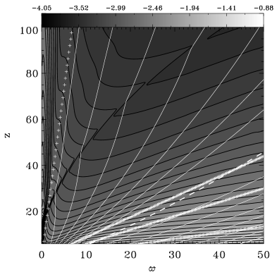
Figure 1: Logarithmic density contours (black lines) and poloidal magnetic fieldlines (white thin lines) are plotted for the final steady-state reached for model $3DB$. The critical surfaces of the initial configuration are given by the plus signs; going counterclockwise we find the slow magnetosonic and slow magnetosonic separatrix (which practically coincide), the Alfvén, the fast magnetosonic, and the fast magnetosonic separatrix surface (FMSS, close to the axis). For the final state, the same surfaces (apart from the FMSS) are indicated with the thick white lines. However, since the analytical equilibrium is preserved in that region, they can hardly be distinguished from those predicted by the steady-state analysis. On the other hand, the FMSS of the final state is not conical any more but diverges from the axis (its position is at the break of the magnetic fieldlines and at the discontinuity of the density). The dashed poloidal fieldline has been selected to compute the integrals of motion shown in Fig. 2.

Figure 2: The integrals of motion (Eqs. [5]-[8]), normalized to unity, are plotted along the poloidal magnetic fieldline (dashed line) indicated in Fig. 1 for the models $1DR$ (left) and $2DB$ (right).

In all cases the initial configurations are maintained and are almost identical: density contours and magnetic fieldlines are being plotted for model $3DB$ (same as model $2DB$ but in higher resolution) in Fig. 1. The surfaces corresponding to the slow magnetosonic and slow magnetosonic separatrix surface, the Alfvén surface, and the fast magnetosonic surface of the final steady state solution are perfectly coinciding with those of the initial analytical solution. This correspondence was also found in GVT06, but it was not so tight: this may be most likely ascribed to the different numerical codes used for the simulations. Conversely, the numerically reshaped fast magnetosonic separatrix (FMSS) diverges from the analytical conical position, and, as will be discussed later, corresponds to a weak shock which can be seen at the density jump and in the break of the poloidal fieldlines.

In Fig. 2, the integrals of motion (Eqs. [5]-[8]) are being shown for models $1DR$ and $2DB$ respectively, normalized to their outer boundary values. The fieldline along which they are computed, begins in a region where $V_{z}<V_{Alfv\acute{e}n;z}$ while it crosses the Alfvénic and fast classical critical surfaces. This is particularly important since a fieldline with its rooting point already in the super-Alfvénic or the super-fast region would give much more similar and hence misleading results for the two cases. It is clear that the integrals of the final solution deviate by less than $\sim 1\%$ when compared to the theoretically expected one, with the exception of the entropy integral $Q$, which shows a rather more sensitive behavior. Note an improvement on the constancy of those integrals as compared to GVT06, where they were found within $\lesssim 15\%$ of their analytical values, again with the exception of $Q$.

Therefore, Fig. 2 – along with the fact that both models $1DR$ and $2DB$ give identical final outcomes – suggests that the results obtained are not really sensitive to the number of boundary conditions imposed. The reason for this, is the fact that the solution is topologically stable and remains close to the initial one. Nevertheless, in order to be physically consistent, the correct number of boundary conditions has to be specified always.

4.1.2 Shock at the FMSS

We now adopt the setup of $2DB$ and perform simulations by effectively increasing the resolution to examine both the behavior and nature of the density and pressure jump observed (models $4DH$, $5DH$, $6DH$).

Figure 3: The density (left) and total pressure (thermal plus magnetic, right) jumps are being plotted for model $6DH$ along the perpendicular to the shock direction centered at the point $x=5,y=33$ (indicated with the diamond in Fig. 4).

Figure 4: The characteristics (thin solid lines) of the fast magnetosonic waves are plotted in a zoomed region around the shock (thick line) for model $5DH$. The point indicated with a diamond is where the quantities of Fig. 3 are plotted. The dashed lines are (clockwise) the analytical FMSS, the fast poloidal critical surface and the Alfvénic one respectively.

Figure 5: The poloidal currents (loci where $\varpi B_{\phi}=\textrm{const}$) of model $5DH$ are plotted. The arrows indicate the direction of the poloidal current density $\@vec{J}_{p}$. A strong current sheet appears tangent to the shock. The dashed lines use the notation of Fig. 4

The discontinuity manifesting in the simulations of the ADO models is identified as a weak shock. This conclusion is supported by taking into account the negative divergence of the velocity (thus denoting the compressional nature of the discontinuity), the jumps appearing on the density and pressure and the fact that the gradients steepen with the increase of the resolution. The density and the total pressure, thermal plus magnetic ($P+B^{2}/2$), are plotted across the shock in Fig. 3. Moreover, the strength of the shock is found to decrease as we move far away from the base, whereas it becomes more and more oblique (see Fig. 1). Consistent with the shock is the break of the poloidal fieldlines, as an effect of the amplification of the tangential component of the poloidal magnetic field. We remark also that the jump in the entropy is very small, though, this is expected by the almost isothermal conditions assumed for the wind ($\gamma=1.05$). However, it has been validated (see discussion on solutions with different polytropic indexes) that by increasing $\gamma\rightarrow\Gamma$ the entropy jump is increasing as well, as expected in adiabatic conditions.

In Fig. 4, selected fast magnetosonic characteristics are plotted. Note that the cones on the left of the shock do not ever cross it but become at best parallel to it. This proves that it corresponds to the numerically readjusted FMSS of the initial exact solution. In particular, the model retains its property of a super-modified-fast solution, and thus a shock develops to preserve the causal disconnection between the flows downstream and upstream. Because the cones constructed by the characteristics of the fast waves in the final superfast region never cross the shock front, it is not surprising that the sub-modified-fast region is not affected at all by the modifications taking place at small polar angles. In other words, the new FMSS behaves like a “wall” preventing the readjustments occurring by the extrapolation close to the axis and downstream of the analytical FMSS to affect the solution upstream of the shock. Such a result is supported by all simulations carried out with the ADO models presented in Table 1.

Furthermore, in Fig. 5 we plot the poloidal currents for model $5DH$. They are counterclockwise upstream and far from the FMSS, they change to clockwise very close and upstream of the FMSS, and finally they change back to counterclockwise downstream of the FMSS. At the FMSS, where the azimuthal magnetic field is discontinuous, we have a strong current sheet with the surface current heading upwards being tangent to the shock. Thus, the currents seem to have a “lightning”, or reverse “N” shape, with their middle part being parallel to the shock. This distribution of the currents, and in particular the direction of the resulting $\@vec{J}_{p}\times\@vec{B}_{\phi}$ force, is consistent with the decollimation and deceleration that the flow experiences as it passes through the shock. Thus, one of the effects of the new FMSS is to bend the streamlines away from the z-axis avoiding the over-collimation property of the original analytical solution. The collimation and decollimation processes that can be derived from such a plot are also discussed in GVT06 (see Fig. 6 there).

4.1.3 Smoothening the flow near the rotational axis

We now proceed to study how different types of extending the solution up to the axis affect the final outcome of the simulation. We adopt the following simple, but diverse enough, extrapolation schemes for the key functions which are shown in Fig. 6 as well:

$$f(\theta)=\left\{\begin{array}[]{rll}\textrm{ I) ($2DB$)}&\textrm{linear extrap.}&\textrm{for }\theta<\theta_{min}\\ \textrm{ II) ($7DS$)}&\textrm{flat extrap.}&\textrm{for }\theta<\theta_{min}\\ \textrm{III) ($8DS$)}&\textrm{smooth extrap.}&\textrm{for }\theta_{FMSS}<\theta\lesssim 7.5^{\circ}\end{array}\right.$$ (32)

Notice that case I) is applied to all but $7DS$ and $8DS$ numerical models of the ADO solution presented in this paper.

Figure 6: Plot of the initial alfvénic mach number, $M$, vs log($\theta$) with the three extrapolation schemes assumed for models I) $2DB$, II) $7DS$ and III) $8DS$.

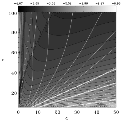
Figure 7: Logarithmic density contours and magnetic poloidal fieldlines for model $8DS$ (case III). The symbols are the same as in Fig. 1. The results for model $7DS$ (case II) are identical with those of models $2DB$ the morphology of which can be seen in Fig. 1.

Figure 8: The integrals of motion (Eqs. [5]-[8]) are plotted along $\varpi$ at $z=50$ for cases I) 2DB (left), II) 7DS (middle) and III) 8DS (right). The dashed line represents the initial setup whereas the solid the final steady-state reached.

Fig. 7 displays the contours of the density for case III) after the simulation has reached a steady state, whereas cases I) and II) give identical results which can be seen in Fig. 1. These first two schemes, which involve modifications only for a small polar angle, display very similar features, despite their different extrapolation assumption. Case III) is of particular importance since the initial solution is sub-modified-fast, i.e. the whole domain is causally connected. However, the shock is still present in the final steady-state reached. Such a result suggests that even by starting from an analytical solution that does not cross the modified-fast critical point, it will probably self-adapt to an “astrophysically correct” solution. With such a term, we mean that it will be consistent with the causal disconnection – of the launching and termination regions – expected to exist in the jet phenomenon. This was somehow anticipated because, for the super-modified-fast extrapolation schemes of cases I) and II), the numerical FMSS is encountered before the analytical one along the flow.

On the other hand, these simulations demonstrate the stability and robustness of the analytical solution since the classical poloidal critical surfaces are not readjusted at all for any of these cases. We conclude that the final steady-state numerical solutions do not show any sensitivity neither on the extrapolation scheme nor to an initial sub-modified-fast solution as far as the criticality condition and the upstream of the shock domain are concerned.

Finally, in order to argue that the extrapolation schemes adopted do not correspond to any physical inconsistencies, we present in Fig. 8 the invariants (Eqs. [5]-[8]) along $\varpi$ at $z=50$ for each case for the initial and final states. Note that case I), which is applied in almost all simulations, is particularly interesting since the inner region is naturally substituted by a lower $\Omega$ mimicking an outflow coming from a slower rotating star.

4.1.4 Lower boundary

We now consider the influence of the choice of $z_{min}$ to the final steady-state reached since the origin is a point where several variables become singular. We construct models $9Dz$ and $10Dz$, by lowering and increasing $z_{min}$ respectively, and we carry out simulations in order to investigate this issue.

Figure 9: Contours of the logarithm of the pressure are being plotted for models $9Dz$, i.e. $z=3$ (left) and $10Dz$, i.e. $z=12$ (right). The values increases towards the axis from a minimum value of -4.0 to a maximum of 0.0, while the iso-baric lines differ by 0.1. The initial and final poloidal critical surfaces are also indicated with the notation already mentioned in Fig. 1.

Fig. 9 shows the pressure contours of models $9Dz$ (left) and $10Dz$ (right); the position of the shock is also evident. Note that in an iso-density contour plot, the shock would not be clearly distinguished because the discontinuity appearing in model $9Dz$ is approximately aligned to the iso-density surfaces, as seen in Fig. 1. Even though the classical critical surfaces of both cases do not present any deviation from the initial model, the region where the shock front develops is considerably different. This result can be understood by noting the following. The characteristics of the fast magnetosonic waves are directly related to the formation of the shock. Therefore, the values of the physical variables in the extrapolated region control its position. Recall that these values are kept fixed since we are in the super-modified fast region. So, we speculate that the closer to the origin we set the bottom boundary, the stronger these extrapolated values will be affected by the steep gradients of the singular origin and the more the characteristics defining the shock will deviate from the analytical FMSS.

4.1.5 Extension to the equator and energetics

We proceed now to extend GVT06 down to the equator and simultaneously examine the effect of different kinds of energy input/output. To achieve the former we adopt spherical coordinates in order to naturally avoid the singularity at the origin, where all critical surfaces coincide. The simulations are performed in the grid with $R\in[10,90]$ and $\theta\in[0,\pi/2-\epsilon]$, utilizing $R\times\theta=[408\times 256]$ uniform zones, where $\epsilon\simeq 1^{\circ}$. We effectively change the way the energy equation is treated by implementing and evolving the following 3 setups: i) applying $\gamma=1.05$ ($11DE$), i.e. according to the analytical solution, ii) assuming $\Gamma=5/3$ ($12DG$) to examine the solution’s behavior to an adiabatic evolution and iii) constraining the system under an isothermal condition ($13DI$).

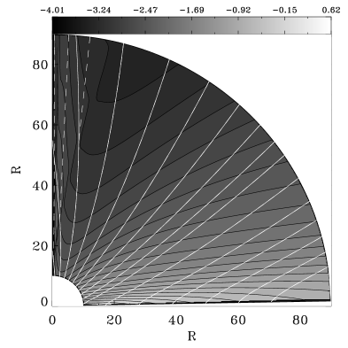
Figure 10: Logarithmic contours of the density (black lines) are being plotted for models $11DE$ (polytropic evolution, left), $12DG$ (adiabatic evolution, middle) and $13DI$ (isothermal evolution, right). The initial (solid) and final (dashed) fieldlines are sketched as well (white lines).

The left panel of Fig. 10 gives the iso-density surfaces and the shape of selected magnetic fieldlines of model $11DE$. As expected, including the equator does not involve any new phenomena, since the analytical solution is well defined there. However, we note that such a computational domain, along with the fixed boundary conditions imposed there, is a physically more consistent choice to describe the MHD outflow, justified by the geometric properties of the disk-star system. Finally, notice that the position of the shock is consistent with the analysis we performed with the cylindrical coordinates, with the role played by $z_{min}$, being now by $R_{min}$.

On the other hand, interesting results are displayed on the middle and right panels of Fig. 10, where selected fieldlines are plotted for the initial setup (solid) and the final numerical steady-state solution (dashed). The plots indicate that even though the polytropic relation is an unavoidable simplification to derive the exact solution of VTST00, it is found to contribute negligibly on the final outcome reached by the numerical evolution. Besides, this is not surprising since the necessary distribution of the pressure needed for constructing such solution is still the same for these cases, with only the energetics during time evolution being different. Such a pressure is crucial in order to force the Alfvénic critical surface to be close to the equator. For a thorough discussion see Ferreira & Casse (Fer04 (2004)).

4.1.6 Long term evolution

Figure 11: Normalized density deviation from its initial value as a function of time at the point $(\varpi,z)=(10,35)$.

Finally, the structural stability argument has to be made concrete by evolving the solution for larger time scales. For that reason we constructed model $14DT$, a case identical to $2DB$, but with its right edge further extended to avoid spurious reflections at the boundaries. Moreover, we choose a point in the upstream of the shock region, i.e. in the sub-modified-fast domain, and plot the deviations of the density from its initial value as a function of time.

It is evident from Fig. 11 that initially ($t\lesssim 2$) the sub-modified-fast solution is being perturbed due to the proper modifications at the axis. However, it converges quickly ($t<5$) to a constant value, roughly $\sim 1.5\%$ different from its initial one. For the rest of the simulation ($5<t<220$) the steady state is perfectly preserved proving its stability. Though, for $t>220$, boundary effects of the imposed outflow conditions of the rightmost and upper boundary have propagated throughout the domain and start to artificially affect the solution. It is worth noting here that the Alfvén velocity is of the order of unity at the lower central region of the computational box. Hence, the Alfvén waves have time to propagate many times before the simulation is brought to a halt.

4.2 The Analytical Stellar Outflow (ASO) solution

The meridionally self-similar solution is in general less complicated to study, since it does not involve any separatrix in the super-Alfvénic region. Therefore, we will mainly investigate here its topological stability and its response towards different restrictions on the evolution of its energy equation. Notice that models $1SR$, $2SL$ and $3SL$ evolve in time with the analytically derived source term participating throughout the whole computational domain. For the rest of the ASO models investigated, the details are given in the following.

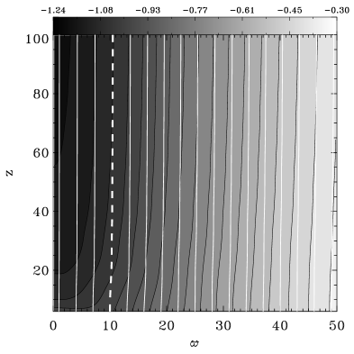
Figure 12: Logarithmic density contours (black lines) are sketched for the final time of the simulation for the model $1SR$ which does not include a sub-Alfvénic region. The magnetic fieldlines are drawn with white lines. The thick dashed one, is chosen to plot along the integrals of motion (Eqs. [5]-[8]; Fig. 14).

4.2.1 Asymptotic configuration

In Fig. 12 we plot the iso-density surfaces along with selected magnetic fieldlines for a super-Alfvénic wind (model $1SR$). Note that in this case we neither have the entropy integral nor the energy one, since for the former there is not any polytropic relation assumed, while for the latter, an explicit energy source term is participating. The initial setup is an exact solution throughout the whole computational domain and hence the final time of the simulation is arbitrarily chosen to be equivalent to the one selected for model $1SR$. The stability of this class of solution can be easily seen in Fig. 14 by the fact that the integrals of motion deviate by only $\lesssim 0.2\%$.

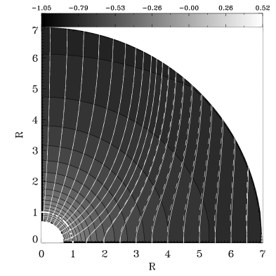
Figure 13: Selected magnetic fieldlines (white lines) are plotted for model $3SL$ which includes a sub-Alfvénic region. Initial analytical solution (solid) and final outcome of the simulations (dashed). The Alfvén critical surface is indicated with a thick dotted-dashed line. The gradients of gray represent the logarithm of the density.

The solution stability has also been successfully validated throughout all its radial range by adopting a logarithmic grid in the radial direction in spherical coordinates (models $2SL$ and $3SL$). Note that model $3SL$ is particularly interesting since $R\in[0.7,7.0]$ with $R_{*}=1$, which implies that both sub-Alfvénic and super-Alfvénic regions are consistently included inside the computational box. Fig. 13 gives the magnetic fieldlines of the final numerical solution which remains identical to the initial analytical one. Therefore, the application of a logarithmic grid allows the approach of the stellar surface, and hence the fixed boundaries imposed are physically justified.

4.2.2 Energetics

It has already been mentioned that one of the main questions posed by the mixing of the two self-similar solutions is on the treatment of the energy equation. Although this will be discussed extensively in a companion work, we carry out simulations here to examine whether the ASO model can reach a steady-state when different energy input/output is included. We firstly address the super-Alfvénic outflow assuming, as in the previous ADO solution, $\gamma=1.05$ (model $4SP$) or the adiabatic case $\Gamma=5/3$ (model $5SG$).

Figure 14: The integrals of motion are plotted along the indicated fieldlines (white dashed line in Fig. 12) for models $1SR$ (left), $4SP$ (middle) and $5SG$ (right).

The outcome of the simulations is a quasi-steady-state that remains very close to the initial solution. With the term quasi-steady, we imply the state when the timescale of the evolution of the system is much larger as compared to the one of the initial more intense readjustments. Especially at the first time steps, the solution is strongly perturbed searching for a new equilibrium due to the different energy source terms imposed. Later on, after the system relaxes, the outer radial regions are found to have remained almost unmodified, whereas, close and along the axis the pressure has increased by roughly half an order of magnitude followed by a slight decrease of the density. This is not surprising, since the analytical explicit energy source term, being taken into account in model $1SR$, is of negative sign there, i.e. corresponds to energy loss. On the contrary, the polytropic case corresponds to a positive input of energy while model $5SG$ to a zero heating/cooling. Hence, the pressure keeps increasing in both cases, due to the absence of the needed cooling, until it reaches a new numerical quasi-equilibrium configuration. The quasi-steady-state reached can be judged by Fig. 14, where the integrals of motion show deviations of $\lesssim 3\%$ after $\sim 100$ Keplerian rotations at the Alfvén radius. This is an expected outcome considering that we are in the super-Alfvénic region: we know that the efficiency of the thermal driving of the flow is concentrated very close to the base, where almost the whole acceleration occurs. This can be seen in Fig. 15 where we plot the energy source term coming from the analytic solution (Eq. [30]). Up to four Alfvén radii, the heating distribution decreases by $\sim 4$ orders of magnitude thus proving its crucial role accelerating the outflow in the inner region. Afterwards, when the flow is propagating with its asymptotic speed, the energetics play a less important role.

One of the properties of these solutions are the oscillations of the fieldlines. The analytical results predict this possibility and we can argue that different energetic processes in the super-Alfvénic region amplifies these features.

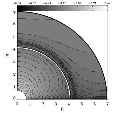
Figure 15: The logarithm of the absolute value of the heating distribution is being plotted (model $3SL$). The thick white line indicates the surface after which the energy input changes sign and becomes cooling. Note that in the inner region, the heating distribution gradually decreases by $\sim 4$ orders of magnitude, while in the outer one by only half.

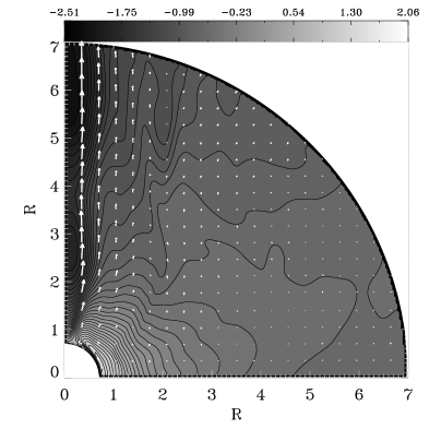
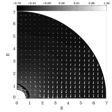
Figure 16: Logarithmic density contours are being plotted for a polytropic evolution ($6SL$ left) and an adiabatic one ($7SL$ right). The velocity vectors overplotted are in the range $[4\cdot 10^{-3},4]$ and $[7\cdot 10^{-7},5\cdot 10^{-1}]$ for the polytropic and adiabatic case, respectively. These models never reach a steady-state.

The results are totally different if the same type of simulations, i.e. polytropic or adiabatic evolution, are performed with the sub-Alfvénic region included (models $6SL$ and $7SL$): in this case there is no steady-state reached. On the left of Fig. 16 a snapshot of the turbulent evolution is displayed when the polytropic assumption with $\gamma=1.05$ is applied. In fact, such a model is able to drive a sporadic low density outflow around the axis, as it can be seen by the velocity vectors.

Conversely, an adiabatic evolution, Fig. 16 on the right, forces the system to collapse towards the star, asymptotically approaching a static atmosphere. This is because the ASO model is thermally driven and when we impose an adiabatic equation of state we effectively switch off all the heating needed to drive the outflow. As expected, the energy processes at the base of meridionally self-similar winds are crucial for their evolution.

5 Summary and conclusions

In this paper we have studied several physical and numerical aspects concerning two classes of the self-similar models, each associated with a disk- and a stellar-wind, in the framework of the upcoming work that combines them to describe a two-component outflow. These analytical solutions (ADO and ASO) were appropriately modified, implemented as initial conditions and evolved in time. Our main conclusions are the following:

• The Analytical Disk Outflow (radially self-similar) solution has been successfully validated for its stability and robustness against several physical and numerical issues. This argument holds true even though the analytical solution was in many cases significantly modified. We have constructed numerical models and carried out simulations a) by assuming the extreme cases of an isothermal and an adiabatic evolution, b) by treating the diverging behavior of the solution at the axis with different kinds of extrapolation schemes, mimicking a stellar wind component and c) by changing the size, resolution and geometry of the computational box.

  In all cases, the poloidal critical surfaces, with the exception of the FMSS, were not readjusted, but rather matched perfectly to their initial position. The numerical solution always maintained the property of the successful crossing of all three critical surfaces producing an outflow causally disconnected from the base. This is achieved with the formation of a shock, corresponding to the numerically readjusted FMSS. In particular, this shock acts as a “wall” protecting the sub-modified-fast magnetosonic regions (source regions of the disk wind) from any perturbations taking place due to the modification of the models close to the axis (e.g. an effective stellar wind). However, the numerically readjusted FMSS (shock) does not coincide with the analytical one, with this departure being dictated by the respective numerical modifications of the models under consideration. A highly significant result is the fact that such a conclusion holds true even if we initialize the simulation with a sub-modified-fast solution, i.e. a solution with its whole domain causally connected. We found that, during the simulation, such a numerical model self-adapts to produce a shock (corresponding to the FMSS), hence no information of the downstream region can travel back to affect the launching region. This implies that even MHD outflow solutions, that do not successfully cross all three critical points, will probably converge to “astrophysically correct” solutions once evolved in time (see also Ferreira Fer97 (1997)).

  On the other hand, the study of GVT06 was successfully extended down to the equator with the help of simulations using spherical coordinates. Furthermore, by adopting different assumptions for the energy source terms, it was shown that the solution is only slightly and accordingly self-modified maintaining all its well defined properties. This is in agreement with the fact that the ADO solution describes essentially a magneto-centrifugally accelerated outflow.

• The Analytical Stellar Outflow (meridionally self-similar) solution, which was validated in time-dependent simulations for the first time, maintained its well-defined equilibrium as expected. Such conclusion is supported by simulations performed with both the super- and sub-Alfvénic regions included. Quite critical are, contrary to disk winds, the effects of the energetics in such thermally driven models. Although different assumptions of the energy equation in the super-Alfvénic domain did not yield any significant modification of the analytical solution, strong variations of the structure of the axial outflows are found if modifications of the heating/cooling mechanisms occur in the initial accelerating region. In particular a polytropic assumption, mimicking isothermal conditions, would produce a turbulent weak outflow, while an adiabatic evolution asymptotically reaches a static atmosphere. We are tempted to relate the heating intermittency and even a switching off in such an ASO solution with the observed variability of accretion-driven YSO outflows.

• All previous statements hold true while being in perfect agreement with physically consistent requirements, such as specifying the correct type of boundary conditions: a) according to the propagation direction of the MHD waves, b) the axisymmetry holding around the axis and c) the constancy of certain physical variables at both a conical surface close to the equatorial plane and a radial one close to the origin, implying the presence of an underlying disk and the stellar surface, respectively. Therefore, the results can safely be trusted since they are not subject to any artificial forcing.

• Last, but certainly not least, is the fact that almost all models of both classes reached a steady- or quasi-steady-state. In this context, the upcoming mixing of the two complementary classes of self-similar solutions in order to study a two-component jet is well founded and promising. The final numerical model will incorporate both proposed scenarios of a pressure-driven outflow (ASO) surrounded by an extended, magneto-centrifugally driven disk wind (ADO). This task is undertaken in the second paper of this series.

- (1) Blandford, R. D., & Payne, D. G. 1982, MNRAS, 199, 883
- (2) Bogovalov, S. V. 1997, A&A, 323, 634
- (3) Bogovalov, S., & Tsinganos, K. 2001, MNRAS, 325, 249
- (4) Burrows, C. J., Stapelfeldt, K. R., Watson, A. M., et al. 1996, ApJ, 473, 437
- (5) Cabrit, S., Edwards, S., Strom, S. E., & Strom, K. M. 1990, ApJ, 354, 687
- (6) Casse, F., & Keppens, R. 2004, ApJ, 601, 90
- (7) Contopoulos, J., & Lovelace, R. V. E. 1994, ApJ, 429, 139
- (8) Dougados, C., Cabrit, S., Lavalley, C., & Ménard, F. 2000, A&A, 357, L61
- (9) Edwards, S., Fischer, W., Hillenbrand, L., & Kwan, J. 2006, ApJ, 646, 319
- (10) Fendt, C. 2006, ApJ, 651, 272
- (11) Ferreira, J. 1997, A&A, 319, 340
- (12) Ferreira, J., Pelletier, G., & Appl, S. 2000, MNRAS, 312, 387
- (13) Ferreira, J., & Casse, F. 2004, ApJ, 601, L139
- (14) Ferreira, J., Dougados, C., & Cabrit, S. 2006, A&A, 453, 785
- (15) Gracia, J., Vlahakis, N., & Tsinganos, K. 2006, MNRAS, 367, 201 (GVT06)
- (16) Hartigan, P., Edwards, S., & Ghandour, L. 1995, ApJ, 452, 736
- (17) Hartigan, P., Edwards, S., & Pierson, R. 2004, ApJ, 609, 261
- (18) Krasnopolsky, R., Li, Z.-Y., & Blandford, R. 1999, ApJ, 526, 631
- (19) Kwan, J., Edwards, S., & Fischer, W. 2007, ApJ, 657, 897
- (20) Meliani, Z., Casse, F., & Sauty, C. 2006, A&A, 460, 1
- (21) Mignone, A. 2005, ApJ, 626, 373
- (22) Mignone, A., Bodo, G., Massaglia, S., et al. 2007, ApJS, 170, 228
- (23) Ouyed, R., Clarke, D., & Pudritz, R. E. 2003, ApJ, 582, 292
- (24) Ray, T. P., Mundt, R., Dyson, J. E., Falle, S. A. E. G., & Raga, A. C., 1996, ApJ, 468, L103
- (25) Sauty, C., & Tsinganos, K. 1994, A&A, 287, 893
- (26) Sauty, C., Trussoni, E., & Tsinganos, K. 2002, A&A, 389, 1068 (STT02)
- (27) Thompson, K. W. 1987, J. Comput. Phys., 68, 1
- (28) Thompson, K. W. 1990, J. Comput. Phys., 89, 439
- (29) Trussoni, E., Tsinganos, K., & Sauty, C. 1997, A&A, 325, 1099
- (30) Tsinganos, K. C. 1982, ApJ, 252, 775
- (31) Tsinganos, K. 2007, Theory of MHD jets and outflows, in Lecture Notes in Physics, Jets from Young Stars: Models and Constraints, J. Ferreira, C. Dougados and E. Whelan (eds.), Springer Verlag, in press
- (32) Tsinganos, K., Sauty, C., Surlantzis, G., Trussoni, E., & Contopoulos, J. 1996, MNRAS, 283, 811
- (33) Vlahakis, N., & Tsinganos, K. 1998, MNRAS, 298, 777
- (34) Vlahakis, N., Tsinganos, K., Sauty, C., & Trussoni, E. 2000, MNRAS, 318, 417 (VTST00)
- (35) Zanni, C., Ferrari, A., Rosner, R., Bodo, G., & Massaglia, S. 2007, A&A, 469, 811