Priority diffusion model in lattices and complex networks

Abstract

We introduce a model for diffusion of two classes of particles ($A$ and $B$) with priority: where both species are present in the same site the motion of $A$’s takes precedence over that of $B$’s. This describes realistic situations in wireless and communication networks. In regular lattices the diffusion of the two species is normal but the $B$ particles are significantly slower, due to the presence of the $A$ particles. From the fraction of sites where the $B$ particles can move freely, which we compute analytically, we derive the diffusion coefficients of the two species. In heterogeneous networks the fraction of sites where $B$ is free decreases exponentially with the degree of the sites. This, coupled with accumulation of particles in high-degree nodes leads to trapping of the low priority particles in scale-free networks.

Diffusion, or the random motion of particles is a most basic mechanism underlying numerous phenomena in nature and technology. While diffusion in periodic regular lattices is rather simple, it is significantly richer in disordered media and complex networks, or when the particles interact with one another. In most studies the particles interact through the excluded volume effect, combined with a potential (as in ‘lattice gas’ models), or through some kind of reaction or transformation of the particles (e.g. Weiss (1994); ben Avraham and Havlin (2000); Kampen (1987); Redner (2001)).

In this paper we introduce a two-species priority diffusion model (PDM): the two species, $A$ and $B$, diffuse independently, but where both species coexist only the high priority particles, $A$, are allowed to move. This problem has several important applications. A frequent case in communication networks is that data packets traverse the networks in a random fashion (e.g. in wireless sensor networks Avin and Brito (2004); Braginsky and Estrin (2002), ad-hoc networks Bar-Yossef et al. (2006); Dolev et al. (2002) and peer-to-peer networks Gkantsidis et al. (2004)). Routers in communication networks handle both high and low priority information packets, such as, for example, in typical multimedia applications. The low priority packets are sent out only after all high priority packets have been sent Kurose and Ross (2004); Tanenbaum (2002), just as in our model.

We solve the priority diffusion model (PDM) analytically for lattices and networks. In lattices and regular graphs both species diffuse in the usual fashion, but the low priority $B$’s diffuse slower than the $A$’s. In heterogeneous scale-free networks the $B$’s get mired in the high degree nodes, effectively arresting their progress. We confirm these conclusions through large-scale computer simulations.

The $A$ and $B$ particles, when selected for motion, hop to one of the nearest neighbor sites, with equal probability. We have investigated two selection protocols. In the site protocol a site is selected at random: if it contains both $A$ and $B$ particles, a high-priority $A$ particle moves out of the site. A particle of type $B$ moves only if there are no $A$’s on the site. If the site is empty, a new choice is made. In the particle protocol a particle is randomly selected: if the particle is an $A$ it then hops out. A selected $B$ hops only if there are no $A$ particles on its site oth . The site protocol describes the case where a selected router sends out packets of information, whereas in the particle protocol agents move independently, describing perhaps the commuting of various individuals. Note that these protocols belong to the general framework of zero-range process with two species of particles (see e.g. Evans and Hanney (2003); Schutz (2003) for factorized steady-state solutions).

We note that the $A$ particles essentially move freely (in both protocols), regardless of the $B$’s. The $B$’s, on the other hand, can move only in those sites that are empty of $A$’s. We begin by considering the number of such sites. We later relate this property to diffusion coefficients of the particles under the priority constraints.

We look first at lattices, or regular graphs, where each site has exactly $z$ nearest neighbors. The number of sites $N\rightarrow\infty$ and for now we focus on a single species, denoting its particle density by $\rho$. Let $f_{j}$ be the average (equilibrium) fraction of sites that contain $j$ particles. Consider a Markov chain process whose states $\{0,1,2,...\}$ are the number of particles in a given site. The $\{f_{j}\}_{j=0,1,2,...}$ are the stationary probabilities of the chain.

For the site protocol, the transition probabilities are:

$$P_{j,j-1}=\frac{1}{N}\;;\qquad P_{j,j+1}=\frac{1-f_{0}}{N}\;.$$ (1)

$P_{j,j}=1-P_{j,j-1}-P_{j,j+1}$ and all other transitions cannot occur. Indeed, for a site to lose a particle it needs to be selected, with probability $\frac{1}{N}$. To gain a particle, a non-empty, one of its $z$ neighbors must be chosen — with probability $(1-f_{0})\frac{z}{N}$ — and this neighbor must send the particle into the original site, with probability $\frac{1}{z}$. Note that the final result is independent of the coordination number $z$. The stationary state satisfies

$$f_{j}=\sum_{i=0}^{\infty}f_{i}P_{ij}\;,$$ (2)

or, in view of (1),

$$f_{j-1}(1-f_{0})+f_{j+1}=f_{j}+f_{j}(1-f_{0})\;,$$ (3)

with the boundary condition $f_{1}=(1-f_{0})f_{0}$. This has the solution $f_{j}=f_{0}(1-f_{0})^{j}$. Imposing particle conservation $\sum_{j=0}^{\infty}jf_{j}=\rho$, we finally obtain:

$$f_{0}^{(\mbox{site})}=\frac{1}{1+\rho}\;.$$ (4)

This agrees nicely with our simulation results (Fig. 1(a), inset).

For the particle protocol the transition probabilities are:

$$P_{j,j-1}=\frac{j}{N\rho}\;;\qquad P_{j,j+1}=\frac{1}{N}\;,$$ (5)

$P_{j,j}=1-P_{j,j-1}-P_{j,j+1}$ and all other transitions are excluded. Indeed, for a site to lose a particle one of its $j$ particles (out of the total $N\rho$) needs to be selected. To gain a particle, one of the $z\rho$ particles that reside, on average, in the neighboring sites has to be chosen, and then hop to the original site (with probability $\frac{1}{z}$). Once again, the result is independent of $z$. This time the boundary condition is $f_{1}=\rho f_{0}$, leading to $f_{j}=f_{0}\frac{\rho^{j}}{j!}$. Imposing the normalization condition $\sum_{j=0}^{\infty}f_{j}=1$, one finally finds

$$f_{0}^{(\mbox{particle})}=e^{-\rho}\;.$$ (6)

In other words, the $\{f_{j}\}$ are Poisson-distributed, with average $\rho$.

We now employ these results for the analysis of priority diffusion, when both species are involved. In regular graphs both species diffuse as in the single-species case, but due to the priority constraints the total time available is split unevenly between the $A$’s and $B$’s. For example, in lattices diffusion is normal, $\left\langle R^{2}\right\rangle=Dt$, as confirmed by simulations (Fig. 1(a)), but with a smaller diffusion coefficient for the hindered $B$’s.

Denote by $P_{A}$ (resp. $P_{B}$) the probability that a moving particle is an $A$ ($B$). In the site protocol, a particle will surely move if we choose a non-empty site (contains $A$, $B$ or both), which happens with probability $1-1/(1+\rho_{A}+\rho_{B})$ (since the particles behave as a single, non-interacting species, if one ignores their labelling, and thus eq. (4) can be applied with $\rho=\rho_{A}+\rho_{B}$). $A$ moves if the selected site contains any number of $A$’s, which happens with probability $\rho_{A}/(1+\rho_{A})$, again, from (4). Therefore, $P_{A}=\frac{\rho_{A}}{1+\rho_{A}}/(1-\frac{1}{1+\rho_{A}+\rho_{B}})$, or:

$$P_{A}=\frac{\rho_{A}(1+\rho_{S})}{(1+\rho_{A})\rho_{S}}\,,\quad P_{B}=\frac{\rho_{B}}{(1+\rho_{A})\rho_{S}}\,,$$ (7)

where $\rho_{S}\equiv\rho_{A}+\rho_{B}$ and we have used $P_{B}=1-P_{A}$ for the second relation. For a single particle in a lattice, $\left\langle R^{2}\right\rangle=t$. Here we have $\left\langle R_{A}^{2}\right\rangle=P_{A}t\equiv D_{A}t$ and thus the diffusion coefficient $D_{A}$ equals $P_{A}$ (similarly, $D_{B}=P_{B}$). Simulations shown in Fig. 1b confirm our predictions (Eq. (7)).

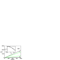
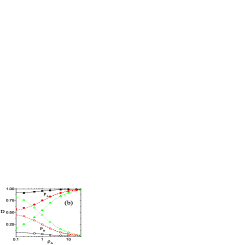
Figure 1: (Color online) PDM in lattices (site protocol). Typical system size is $10^{4}$ sites and time is $10^{3}$ steps. (a) Mean square displacement of a particle $\left\langle R^{2}\right\rangle$ (averaged over all particles and realizations) as a function of time. In one time step each particle moves on average once. Black squares are for densities $\rho_{A}=\rho_{B}=10$, green triangles for $\rho_{A}=\rho_{B}=1$. Inset: $f_{0}$ as a function of density. The solid curve represents Eq. (4), while symbols denote simulation results. (b) Diffusion coefficients, $D$ ($P_{A}$ full symbols, $P_{B}$ empty symbols), as a function of $\rho_{A}$. Black squares are for $\rho_{A}=10\rho_{B}$, red circles for $\rho_{A}=\rho_{B}$ and green triangles for $\rho_{A}=0.1\rho_{B}$. The continuous ($P_{A}$) and dotted ($P_{B}$) curves represent Eq. (7).

For the particle protocol, denote the ratio of free $B$ particles (that do not share a site with $A$’s) to all $B$ particles by $r$. Any particle will surely move except for the case when a non-free $B$ particle was chosen (which happens with probability $\rho_{B}/\rho_{S}\cdot(1-r)$). $B$ moves whenever a free $B$ is chosen, with probability $\rho_{B}/\rho_{S}\cdot r$. Therefore we find:

$$P_{B}=\frac{r\rho_{B}/\rho_{S}}{1-(1-r)\rho_{B}/\rho_{S}},$$ (8)

and $P_{A}=1-P_{B}$.

Had the density of $B$’s been independent of the $A$’s then $r$ would simply be the fraction of sites empty of $A$, or $r=e^{-\rho_{A}}$. However, due to the priority constraints $B$’s tend to stick with the $A$’s, so that $r\lesssim e^{-\rho_{A}}$. The ratio $r$ can be obtained analytically for low densities, if we assume that a single site cannot contain more than one $A$ or $B$. We use again a Markov chain formulation, but now with just four possible states to each site: $\{\phi,A,B,AB\}$ (state $A$ corresponds to a site having one $A$ particle, and similarly for the other states). We write the transition probabilities as before, to first order in the densities:

$$P_{\phi,A}=\frac{\rho_{A}}{N\rho_{S}}\;;\quad P_{\phi,B}=\frac{\rho_{B}}{N\rho_{S}}\;;$$

$$P_{A,\phi}=\frac{1}{N\rho_{S}}\;;\quad P_{A,AB}=\frac{\rho_{B}}{N\rho_{S}}\;;$$

$$P_{B,\phi}=\frac{1}{N\rho_{S}}\;;\quad P_{B,AB}=\frac{\rho_{A}}{N\rho_{S}}\;;$$

$$P_{AB,B}=\frac{1}{N\rho_{S}}\;.$$ (9)

Unindicated transition probabilities are zero, and the diagonal accounts for normalization $P_{x,x}=1-\sum_{y\neq x}P_{x,y}$. The justification is similar to that of Eq. (5). For a site to lose a particle, this particle needs to be chosen out of a total of $N\rho_{S}$ particles. For a site to gain an $A$, one of the $z\rho_{A}$ particles that reside, on average, in the neighboring sites has to be chosen (out of $N\rho_{S}$), and then sent to the target site, with probability $\frac{1}{z}$ (and likewise for gaining a $B$). The priority constraint is taken into account by forbidding the transition $AB\rightarrow A$.

From the stationary probabilities of the chain (Eq. (2)) we derive $r$ to first order:

$$r=\frac{f_{B}}{f_{B}+f_{AB}}=1-2\rho_{A}+{\cal O}(\rho^{2})$$ (10)

($\rho$ stands for either $\rho_{A}$ or $\rho_{B}$). To obtain the next order, allowed states can have two particles of each type, and we take into account that when a $B$ is chosen it actually hops only with probability $r$ (using its first-order expression, Eq. (10)). We thus find

$$r=1-2\rho_{A}+\frac{13}{4}\rho_{A}^{2}+{\cal O}(\rho^{3})\;.$$ (11)

Surprisingly, $r$ does not depend on $\rho_{B}$, at least to second order. In fact, our simulations suggest that $r$ is independent of $\rho_{B}$ for all densities (Fig. 2(a)). For large $\rho_{A}$ we have $r\rightarrow e^{-\rho_{A}}$, since free $B$’s become extremely rare. The diffusion coefficients obtained on substituting Eq. (11) in (8) compare quite nicely with simulations (Fig. 2(b)).

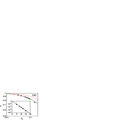
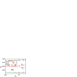
Figure 2: (Color online) PDM in lattices (particle protocol). Simulation parameters are same as in Fig. 1. (a) Fraction $r$ of free $B$’s as a function of $\rho_{A}$ for the cases $\rho_{A}=\rho_{B}$ (black squares), $\rho_{A}=0.2\rho_{B}$ (empty red circles), and $\rho_{A}=5\rho_{B}$ (green triangles), compared to the result of Eq. (11) (solid line). $r$ is smaller than $e^{-\rho_{A}}$ (dotted red line) since $B$ particles tend to stick with the $A$’s. Inset: Large $\rho_{A}$ regime, where $r$ tends to $e^{-\rho_{A}}$ ($\rho_{B}=\rho_{A}$). (b) Diffusion coefficients ($P_{A}$ full symbols, $P_{B}$ empty symbols) as a function of $\rho_{A}$ for the cases $\rho_{A}=10\rho_{B}$ (black squares), $\rho_{A}=\rho_{B}$ (red circles), and $\rho_{A}=0.1\rho_{B}$ (green triangles). The continuous ($P_{A}$) and dotted ($P_{B}$) curves represent Eqs. (8) and (11). Inset shows $P_{B}$ (red circles) for large $\rho_{A}$. The $B$ particles diffuse much slower here compared to the site protocol (continuous red line) due to the exponential decrease in the number of empty sites.

We now turn to heterogeneous networks, where the degree $k$ varies from site to site. We focus on two explicit models: Erdős-Rényi (ER) random graphs Erdős and Rényi (1959); Bollobás (1985), where the degrees of the nodes are narrowly (Poisson) distributed, and scale-free (SF) networks, recently discovered to best describe a wide variety of natural and man-made systems, and in particular many communication networks such as the Internet. In SF nets the degree distribution is broad, characterized by a power-law tail $P(k)\sim k^{-\gamma}$, when usually $2<\gamma<3$ Albert and Barabási (2002); Pastor-Satorras and Vespignani (2004); Dorogovtsev and Mendes (2003); Newman (2003).

We analyze the particle protocol only — the site protocol yields similar results, as we confirmed through computer simulations. We wish to find the fraction of empty sites of degree $k$, $f_{0}^{(k)}$. As before, consider a network with only one particle species and define a Markov chain on the states $\{0,1,2...\}$ for the number of particles in a given site of degree $k$. The stationary probabilities are $f_{j}^{(k)}$. It can be shown that the chain has the transition probabilities:

$$P_{j,j-1}=\frac{j}{N\rho}\;;\quad P_{j,j+1}=\frac{k}{\left\langle k\right\rangle}\frac{1}{N}\;,$$ (12)

$P_{j,j}=1-P_{j,j-1}-P_{j,j+1}$ and all other probabilities are zero. Intuitively, this is the same as Eq. (5), except that here a site may gain a particle from any of its $k$ neighbors, and the neighbor delivers the particle to the target site with probability $\frac{1}{\left\langle k\right\rangle}$ ($\left\langle k\right\rangle$ is the average degree of the net). Solving for the stationary probabilities while keeping in mind that $\sum_{j}f_{j}^{(k)}=1$ one finds

$$f_{j}^{(k)}=f_{0}^{(k)}\frac{\left(\frac{\rho k}{\left\langle k\right\rangle}\right)^{j}}{j!}\;;\quad f_{0}^{(k)}=\exp\left({-\frac{\rho k}{\left\langle k\right\rangle}}\right)\;.$$ (13)

Note that for regular graphs, when all sites have the same degree, this reduces to Eq. (6), $f_{0}=e^{-\rho}$. Also, the total number of particles in a site of degree $k$ is thus $\sum_{j=0}^{\infty}jf_{j}^{(k)}=\frac{\rho k}{\left\langle k\right\rangle}\propto k$, as is well known for random walks on networks Noh and Rieger (2004). For the full network, $f_{0}=\sum_{k=1}^{\infty}f_{0}^{(k)}P(k)$ k_ . In particular, for ER graphs,

$$f_{0}=\sum_{k=1}^{\infty}e^{-\frac{\rho k}{\left\langle k\right\rangle}}e^{-\left\langle k\right\rangle}\frac{\left\langle k\right\rangle^{k}}{k!}=e^{-\left\langle k\right\rangle}(e^{\left\langle k\right\rangle e^{-\frac{\rho}{\left\langle k\right\rangle}}}-1)\,.$$ (14)

The agreement between these predictions and simulations is shown in Fig. 3(a).

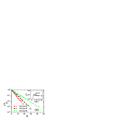
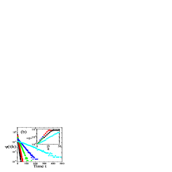
Figure 3: (Color online) PDM in networks. Typical system size for both ER and SF is $10^{4}$ nodes, Internet is 21955 nodes and time is $10^{4}$ MCS. SF networks were generated using the Molloy-Reed algorithm Molloy and Reed (1998). (a) Fraction of empty sites in ER (empty symbols) and SF (full symbols) networks as a function of site degree. The curves follow Eq. (13). Inset: Fraction of empty sites for ER vs. $\left\langle k\right\rangle$ for fixed density $\rho=1$. The continuous curve represents Eq. (14). (b) Distribution of waiting times for $B$ particles for nodes of various degrees ($k=2,4,7,10,15$, left to right) in SF networks ($\gamma=3,m=2$). Inset: $\left\langle t\right\rangle$ as a function of k. Shown are: SF and ER networks with $\left\langle k\right\rangle=4$ (black squares and green triangles), and $\left\langle k\right\rangle=3$ (red circles and blue triangles), and the Internet Carmi et al. (2007) (cyan diamonds). Solid curves represent the theoretical $\left\langle t(k)\right\rangle=\exp(\rho_{A}k/\left\langle k\right\rangle)$. Plateau for large $k$ results from finite simulation time.

Consider now priority diffusion. Define that in one time step each particle has on average one moving attempt. On average, at every time step a $B$ particle (in a node of degree $k$) has a probability $\exp(-\rho_{A}k/\left\langle k\right\rangle)$ to be able to jump out (Eq. (13)). This results in a distribution of waiting times (for a $B$ particle)

$$\psi_{k}(t)=\frac{1}{\tau}e^{-t/\tau}\;,$$ (15)

where $\tau\equiv\left\langle t(k)\right\rangle=\exp(\rho_{A}k/\left\langle k\right\rangle)$ is simply the inverse of the probability for the site to be empty of $A$’s (Fig. 3(b)).

The exponentially long waiting time (in the degree $k$) means that in heterogeneous networks such as scale-free nets — where the degrees may span several orders of magnitude — the $B$ particles get mired in the hubs (high degree nodes). The problem is exacerbated by the fact that the $B$ particles are drawn to the hubs even in the absence of $A$’s: the presence of $A$’s only amplifies this tendency, because of the positive correlation between the concentrations of the two species. Thus, while the concentration of the $A$’s is proportional to $k$, it can be shown that the concentration of the $B$’s is proportional to $k\exp(\rho_{A}k/\left\langle k\right\rangle)$. In large scale-free nets the $B$’s collect at the hubs, which results in extremely long waiting times and practical halting of particles diffusion.

In conclusion, we have introduced and analyzed a model of priority diffusion, involving two species, where the particles of the preferred species always move ahead of the other. In regular graphs and lattices diffusion of each of the species is similar to that of a single (non-interacting) species on the same substrate, but the overall diffusion rate of the preferred species is significantly faster: we have provided exact expressions for the rate ratios in this case. In heterogeneous nets, we have shown that the slow-species particles tend to be collected in the high degree nodes, where their waiting time for clearing the site increases exponentially with the degree of the site. In scale-free nets where the degrees span several orders of magnitude the slow species progress is effectively arrested.

Our calculations for heterogeneous networks are mean-field in character, in that we ignore possible correlations between the degrees of neighboring nodes. This assumption is valid, though, for ER random graphs and for maximally random networks, such as Molloy-Reed SF nets Molloy and Reed (1998). The possible effect of degree-degree correlations remains a subject for future research.