Asymptotic description of solitary wave trains in fully nonlinear shallow-water theory

Abstract

We derive an asymptotic formula for the amplitude distribution in a fully nonlinear shallow-water solitary wave train which is formed as the long-time outcome of the initial-value problem for the Su-Gardner (or one-dimensional Green-Naghdi) system. Our analysis is based on the properties of the characteristics of the associated Whitham modulation system which describes an intermediate “undular bore” stage of the evolution. The resulting formula represents a “non-integrable” analogue of the well-known semi-classical distribution for the Korteweg-de Vries equation, which is usually obtained through the inverse scattering transform. Our analytical results are shown to agree with the results of direct numerical simulations of the Su-Gardner system. Our analysis can be generalised to other weakly dispersive, fully nonlinear systems which are not necessarily completely integrable.

1 Introduction

It is widely appreciated that, although completely integrable systems may successfully capture many important features of nonlinear dispersive wave propagation, they may fail to provide an adequate description of large amplitude waves. Consequently, significant efforts have recently been directed towards the derivation and analysis of relatively simple models, enabling the quantitative description of the propagation of fully nonlinear waves. Although such “intermediate” models are typically not integrable using an inverse scattering transform (IST), they often provide the possibility of obtaining important particular solutions, as well as having other advantages compared to the full physical system from the viewpoint of numerical simulations.

One such system, the so-called Green-Naghdi (GN) equations, describes large-amplitude shallow water waves [1] and also appears in a number of other fluid dynamics contexts, such as “continua with memory” [2], solar magnetohydrodynamics [3], bubbly fluid flows [4] and the dynamics of short capillary-gravity waves [5]. The two-layer versions of the GN system [6, 7, 8] provide a broad field for the modelling of large amplitude interfacial waves. It should be noted that the one-dimensional version of the GN system, which is the main subject of this paper, was originally derived by Su and Gardner [9] using a long-wave asymptotic expansion of the full Euler equations for irrotational flow (see also El, Grimshaw & Smyth [10]), while the original 2D GN system was derived using the “directed fluid sheets” theory, which does not require a formal asymptotic expansion, but instead imposes the condition that the vertical velocity has only a linear dependence on the vertical $(z)$ coordinate, and simultaneously assumes that the horizontal velocity is independent of $(z)$. In this paper we shall use the term SG system which appears historically more correct, at least for one-dimensional dynamics. The SG system has the form

$$\eta_{t}+(\eta u)_{x}=0\,,$$ (1)

$$u_{t}+uu_{x}+\eta_{x}=\frac{1}{\eta}\left[\frac{1}{3}\eta^{3}(u_{xt}+uu_{xx}-(u_{x})^{2})\right]_{x}\,,$$

where, in the context of shallow-water waves, $\eta$ is the total depth and $u$ is the layer-mean horizontal velocity; all variables are non-dimensionalised by their typical values. The first equation is the exact equation for conservation of mass and the second equation can be regarded as an approximation to the equation for conservation of horizontal momentum. The system (1) has the typical structure of the well-known Boussinesq-type systems for shallow water waves, but differs from them in retaining full nonlinearity in the leading-order dispersive term on the right-hand side of (1). We stress that there is no limitation on the amplitude assumed in the derivation of (1). This, along with the appearance of this system in different physical contexts, suggests that equations (1) represent an important mathematical model for understanding general properties of fully nonlinear fluid flows beyond the strict shallow-water limit. For this reason, it is instructive to study its solutions for the full range of amplitudes, although in the particular context of shallow-water waves the system (1), as for any layer-mean model, is unable to reproduce the effects of wave overturning and becomes nonphysical for amplitudes greater than some critical value.

The system (1) has a solitary wave solution of the form

$$\eta=\eta_{0}+a\ \hbox{sech}^{2}\left(\frac{\sqrt{3a}}{\eta_{0}\sqrt{\eta_{0}+a}}(x-ct)\right)\,,$$ (2)

where the solitary wave speed $c$ is connected to the amplitude $a$ by the relationship

$$c=u_{0}+\sqrt{\eta_{0}+a}\,.$$ (3)

Here $u_{0}$ and $\eta_{0}$ are the background flow parameters. We note that formula (3) appears in Rayleigh [11].

The asymptotic reduction of the SG system (1) for weakly nonlinear waves is obtained by using the standard scaling $\eta=\eta_{0}+\delta\zeta$, $u=u_{0}+\delta U$, $x-c_{0}t\to\delta^{-1/2}x$, $t\to\delta^{-3/2}t$, where $\delta$ is a small parameter and $c_{0}=u_{0}+\sqrt{\zeta_{0}}$ is the linear longwave speed. For uni-directional propagation, this leads to the KdV equation (see, for instance, Johnson [12])

$$\zeta_{t}+\frac{3}{2}\zeta\zeta_{x}+\frac{1}{6}\zeta_{xxx}=0\,.$$ (4)

With the further scaling $x^{\prime}=\sqrt{6}x\,,t^{\prime}=\sqrt{6}t\,,v=3\zeta/2$, (4) reduces to the standard KdV form

$$v_{t}+vv_{x}+v_{xxx}=0\,,$$ (5)

on omitting the primes. Then if one considers sufficiently rapidly decaying positive initial data for (5)

$$\qquad v(x,0)=v_{0}(x)\geq 0\,,\qquad v_{0}\to 0\ \ \hbox{as}\ \ |x|\to\infty\,,$$ (6)

where $v_{0}(x)$ is a continuous “one-hump” function, then as $t\to\infty$ the solution asymptotically consists of a finite number of solitons plus dispersive radiation.

The associated linear spectral problem for (5) is given by the Schrödinger equation

$$6\psi_{xx}+(v(x,t)-\lambda)\psi=0\,.$$ (7)

Note that this is in non-standard form due to the factor $6$ in the first term. Then the parameters of the solitons and the radiation are found from the IST using the initial condition $v_{0}(x)$ (6) for $v$ in (7). In particular, a soliton with amplitude $a_{n}$ corresponds to the eigenvalue $\lambda_{n}=a_{n}/2$ of the Schrödinger operator.

If one considers a large-scale initial distribution such that $\epsilon=1/(A^{1/2}w)\ll 1$, where $A\propto\max v_{0}$, and $w$ is the typical width of $v_{0}(x)$, then the contribution of the radiation is exponentially small in $\epsilon$ and as $t\to\infty$ the asymptotic outcome consists only of a large ($N\propto\epsilon^{-1}$) number of solitons, whose amplitudes can be found from the Bohr-Sommerfeld semi-classical quantization rule,

$$\frac{1}{\sqrt{6}}\int_{x_{1}}^{x_{2}}\sqrt{v_{0}(x)-\lambda}\ dx=\pi(n-\frac{1}{2})\,,\quad n=1,2,3,\dots,N\,.$$ (8)

Here the integral is taken between the turning points $x_{1,2}$ defined as the roots of the equation $v_{0}(x)=\lambda$. For every given $n$ formula (8) yields a bound state $\lambda_{n}>0$;   $A\approx\lambda_{1}>\lambda_{2}>\dots>\lambda_{N}\approx 0$ with $N$ the total number of bound states in the potential $v_{0}(x)$. In the KdV context the distribution (8), through $a_{n}=2\lambda_{n}$, gives the amplitude of the $n$-th soliton in the soliton train as $t\to\infty$. For the largest amplitude soliton we have the classical result

$$a_{\max}=2\lambda_{1}=2A\,.$$ (9)

On the other hand, for a given $\lambda\in[0,A]$, the formula (8) determines the total number of bound states $n$ in the spectral interval $(\lambda,A)$ as

$$n=\hbox{i.p.}\ (F(\lambda)+\frac{1}{2})\,,\qquad F(\lambda)=\frac{1}{\sqrt{6}\pi}\int_{x_{1}}^{x_{2}}\sqrt{v_{0}(x)-\lambda}\ dx\,.$$ (10)

Here “$\hbox{i.p.}\ (\cdot)$” denotes the integer part.

For large $n$ the bound states are located close to each other and we can introduce a continuous amplitude function $a=2\lambda$. Then differentiating (8) with respect to $a$, one obtains the distribution function for soliton amplitudes in the train

$$f(a)=\left|\frac{dn}{da}\right|=\frac{1}{4\pi}\frac{1}{\sqrt{6}}\int_{x_{1}}^{x_{2}}\frac{dx}{\sqrt{v_{0}(x)-a/2}}\,,$$ (11)

so that $f(a)da$ yields the number of solitons having amplitudes in the interval $(a,a+da)$. The total number of solitons in the soliton train is estimated by setting $\lambda=0$ in (8) (alternatively, one can integrate $f(a)$ from $0$ to $a_{\max}$)

$$N\cong\frac{1}{\sqrt{6}\pi}\int_{-\infty}^{+\infty}\sqrt{v_{0}(x)}\ dx\sim A^{1/2}w\,.$$ (12)

The distribution (11) was originally introduced into soliton theory by Karpman [13] (see also Whitham [14] and Karpman [15]). More recently, distributions of this type have been obtained, also from the associated linear spectral problem, for the defocusing nonlinear Schrödinger equation [16] and for the Kaup-Boussinesq system [17].

One can see that integrability of the KdV equation plays a crucial role in the derivation of the formulae (8)–(12) through the eigenvalue problem for the associated linear Schrödinger equation (7). At the same time one can observe that the formulae obtained correspond to the semi-classical approximation and that this very approximation can be applied directly to the KdV equation, by-passing the IST formalism. It is well-known (see Lax and Levermore [18]) that the semi-classical limit of the KdV equation with decaying initial data leads to the Whitham modulation system, which can be derived by a direct averaging of the KdV conservation laws over nonlinear wavepackets [19] or from a multiple-scale perturbation analysis [20, 21]. Therefore one could expect that the results (9)–(12) could be obtained within the framework of the modulation theory alone. Indeed, it was shown in Gurevich et al [22] and El & Grimshaw [23] that the long-time asymptotics of exact solutions to the KdV-Whitham equations with decaying initial data agrees, to first order in $t^{-1}$, with Karpman’s formula (11). Still, modulation solutions in the cited papers rely on the integrability of the KdV equation as they employ the presence of Riemann invariants for the associated Whitham system [19], and this latter property is due to the unique finite-gap spectral structure of periodic (or, more-generally, quasi-periodic) solutions of the KdV equation [24].

An important theme in the original work of Whitham [19] is that, unlike the IST, the nonlinear modulation approach can be applied to nonintegrable dispersive systems provided a minimal structure is present, that is the existence of periodic solutions characterised by a certain number of parameters, and the availability of a limited number of conservation laws. The resulting modulation system consists of hydrodynamic-type equations and is hyperbolic in many cases, which implies that it can be treated using classical methods of characteristics theory (see, for instance, Courant & Hilbert [25]). This opens the possibility of obtaining some analytical results for non-integrable dispersive wave systems in the framework of modulation theory.

Indeed, it was recently shown in El [26] that the availability of a number of important exact results for the single-phase modulation theory is, in fact, due to certain very general properties of modulation systems and is not connected with the presence of the Riemann invariant structure. These properties have been used in El, Grimshaw & Smyth [10] to derive the main parameters of large-amplitude shallow-water undular bores evolving from an initial step for the SG system (1). In the present paper, we extend the modulation analysis of El [26] and El, Grimshaw & Smyth [10] to obtain an analogue of Karpman’s formula (11) and its consequences (9) and (12) for the SG system for an initial disturbance in depth and velocity that decays at infinity. Our approach is based on an assumption, confirmed by numerical solutions, that the main qualitative features of the KdV evolution of large-scale disturbances, such as the formation of a single-phase undular bore and its further evolution into a solitary wave train with a negligibly small contribution of the linear radiation, remain present in the SG model. Our analytical results will be supported by comparison with full numerical solutions of the SG system.

2 Asymptotic formula for the KdV equation derived from modulation theory

2.1 Characteristic integrals of the modulation system

It is instructive to start with a demonstration of our general approach to an asymptotic description of solitary wave trains by using the KdV equation as a “test” example. Our ultimate goal here is to derive Karpman’s formula (11) without invoking the integrability properties of the KdV equation and its modulation system. This derivation will then serve as a prototype for calculations for the SG system, which is genuinely non-integrable.

We consider the initial-value problem (5) and (6). Without being too restrictive, we also assume that $v_{0}(x)=0$ for $x\geq 0$, which will simplify the following analysis. As before, we consider a large-scale initial disturbance, so that $(A^{1/2}w)^{-1}\ll 1$, where $A=\max{(v_{0})}$ and $w$ is the characteristic width of the initial hump.

The wave evolution from (5) and (6) leads to wave breaking at some $t=t_{b}$, which can be taken to be $t_{b}=0$ without loss of generality, which is then resolved by an undular bore (which is also often called a dispersive shock wave), which is an expanding nonlinear modulated wave train with a distinctive spatial structure. Near the leading edge of the undular bore the oscillations appear to be close to successive solitary waves, while in the vicinity of the trailing edge they are nearly linear. An asymptotic similarity modulation solution for the undular bore evolving from an initial distribution in the form of a sharp step was first obtained by Gurevich and Pitaevskii (GP) [27] using the Whitham method of averaging over periodic nonlinear wavetrains [14, 19] and then rigorously recovered in the framework of the semiclassical IST formalism by Lax, Levermore and Venakides (see their review [18] and references therein). In contrast to the Lax-Levermore-Venakides global construction, the direct modulation approach of GP does not rely on the IST and thus has the advantage of potential applicability to non-integrable systems. This advantage was realised in El [26] for the simplest class of problems with step-like initial conditions where the modulation solution for the undular bore represents an expansion fan, similar to the GP solution.

For the case of positive initial data, which decay at infinity, the whole initial disturbance decomposes, at very large times $t\gg\varepsilon^{-1}$, into a chain of solitons with a certain amplitude distribution. As was mentioned in the Introduction, the semi-classical IST approach leads to Karpman’s formula (11) for this distribution. However, it transpired that the same result can be obtained using the derivation of the intermediate modulation solution for the undular bore and then considering its long-time asymptotic behaviour [22, 23]. In this connection it should be mentioned that the modulation dynamics in these problems with decaying initial data is not self-similar, so the original Gurevich-Pitaevskii [27] theory required significant development in order to be applied to such problems. It transpires that further development is required to extend modulation analysis to non-integrable systems with decaying initial data. Below we present the GP formulation for the KdV equation in a form convenient for further generalistion to non-integrable systems.

The local waveform of the undular bore is described by the single-phase periodic solution of the KdV equation travelling with constant velocity $c$, that is $v(x,t)=v(\theta)$, $\theta=x-ct$. This solution is specified by the ordinary differential equation

$$(v_{\theta})^{2}=Q(v)\,,\quad Q(v)=\frac{1}{3}(v-v_{1})(v-v_{2})(v_{3}-v)\,,\quad v(\theta+2\pi/k)=v(\theta)\,,$$ (13)

$v_{3}\geq v_{2}\geq v_{1}$ being constants of integration. The phase velocity $c$, the amplitude $a$, the wavenumber $k$ and the mean $\overline{v}$ are expressed in terms of the polynomial roots $v_{j}$ as

$$c=\frac{1}{3}(v_{1}+v_{2}+v_{3}),\quad a=v_{3}-v_{2},\quad\quad k={\pi}\left(\int\limits^{v_{3}}_{v_{2}}\frac{dv}{\sqrt{Q(v)}}\right)^{-1},\quad\overline{v}=\frac{\pi}{k}\int\limits^{v_{3}}_{v_{2}}\frac{vdv}{\sqrt{Q(v)}},$$ (14)

while the wave frequency is $\omega(\overline{v},k,a)=kc$. When $a\to 0$ the solution of (13) turns into small amplitude harmonic waves with the dispersion relation

$$\omega_{0}(\overline{v},k)=\omega(\overline{v},k,0)=k\overline{v}-k^{3}\,.$$ (15)

In an opposite extreme, when $k\to 0$, the travelling wave $u(\theta)$ transforms into a soliton with its velocity depending on the amplitude as

$$c_{sol}=\overline{v}+\frac{a}{3}$$ (16)

If one allows slow dependence of $v_{1}$, $v_{2}$ and $v_{3}$ or, equivalently, $\overline{v}$, $k$, and $a$ on $x$ and $t$, one arrives at the modulation system which can be derived by averaging two of the KdV conservation laws over the periodic wave family (13)

$$\frac{\partial\overline{v}}{\partial t}+\frac{\partial}{\partial x}\left(\frac{\overline{v^{2}}}{2}\right)=0\,,\quad\frac{\partial}{\partial t}\left(\frac{\overline{v^{2}}}{2}\right)+\frac{\partial}{\partial x}\left(\overline{\frac{v^{3}}{3}-\frac{v_{\theta}^{2}}{2}+vv_{\theta\theta}}\right)=0\,$$ (17)

and then closing (17) with the equation for “conservation of waves” (see Whitham [14])

$$\frac{\partial k}{\partial t}+\frac{\partial\omega(\overline{v},k,a)}{\partial x}=0\,.$$ (18)

We note that the detailed expressions for the averages in (17) will not be needed. To describe the evolution of modulations in an undular bore the system (17) and (18) must be equipped with matching conditions ensuring continuity of the mean $\overline{u}$ at the undular bore edges $x^{\pm}(t)$ [27]

$$\begin{array}[]{l}x=x^{-}(t):\qquad a=0\,,\ \ \overline{v}=\beta^{-}(t)\,,\\ x=x^{+}(t):\qquad k=0\,,\ \ \overline{v}=\beta^{+}(t)\,.\end{array}$$ (19)

Here $\beta^{\pm}(t)=\beta(x^{\pm}(t),t)$, where $\beta(x,t)$ is the solution of the Hopf equation

$$\beta_{t}+\beta\beta_{x}=0\,,\quad\beta(x,0)=v_{0}(x)\,,$$ (20)

which represents the dispersionless limit of the KdV equation (4) and is valid outside the oscillatory region. As we have assumed that $v_{0}(x)=0$ for $x\geq 0$, we have $\beta^{+}=0$.

The trailing $x^{-}(t)$ and the leading $x^{+}(t)$ edges of the undular bore represent free boundaries defined by the kinematic conditions

$$\frac{dx^{-}}{dt}=c_{g}(\beta^{-},k^{-})\,,\qquad\frac{dx^{+}}{dt}=c_{sol}(\beta^{+},a^{+})\,,$$ (21)

where $c_{g}=\partial\omega_{0}/\partial k$ is the group velocity of linear waves and $k^{-}=k^{-}(t)=k(x^{-}(t),t)$, $a^{+}=a^{+}(t)=a(x^{+}(t),t)$. It is important to note that, according to general properties of quasi-linear hyperbolic systems (see, for instance, Courant & Hilbert [25]), the curves $x^{\pm}(t)$, being the lines which match two analytically different solutions, must coincide with characteristics of the modulation system (17) and (18). Indeed, as we shall see, the kinematic conditions (21) and the requirement that the undular bore boundaries must be characteristics of the modulation system are equivalent.

We now consider the modulation equations in two distinguished limits: as $a\to 0$ and as $k\to 0$— corresponding to the wave regimes at the trailing and the leading edges of the undular bore respectively. When $a\to 0$ the oscillations do not contribute to the averaging, so $\overline{F(v)}=F(\overline{v})$, where $F(v)$ is an arbitrary function, and the modulation system must reduce to (see El [26] for details)

$$a=0\,,\qquad\overline{v}_{t}+\overline{v}\cdot\overline{v}_{x}=0\,,\qquad k_{t}+(\omega_{0}(\overline{v},k))_{x}=0\,.$$ (22)

The system (22) has two families of characteristics, $dx/dt=\overline{v}$ and $dx/dt=\partial\omega_{0}/\partial k$. The first family is consistent with the characteristics of the “external” Hopf equation (20) which transfers initial data from the $x$ axis into the undular bore region in the $(x,t)$-plane, while one of the characteristics of the second family specifies the trailing edge of the undular bore (see the first kinematic condition (21)). Then, according to the general properties for the prescription of Cauchy data on characteristics (see, for instance, Whitham [14]), one cannot specify the values of $\overline{v}$ and $k$ at the trailing edge independently. Of course, a similar statement is true for the leading edge as well, and this is why the matching conditions (19) are sufficient to determine the evolution of an undular bore regardless of the fact that they involve less variables than the modulation system (17). The admissible combinations of the values of $\overline{v}$ and $k$ on a characteristic with $a=0$ are found by a substitution of $k=k(\overline{v})$ into (22), which leads to the ordinary differential equation

$$\qquad\frac{dk}{d\overline{v}}=\frac{\partial\omega_{0}/\partial\overline{v}}{\overline{v}-\partial\omega_{0}/\partial k}.$$ (23)

Substituting the linear dispersion relation (15) into (23) one readily obtains the characteristic integral

$$k(\overline{v})=\sqrt{\frac{2}{3}(\overline{v}-\lambda_{1})}\,,$$ (24)

where $\lambda_{1}$ is an arbitrary constant.

We now consider the soliton limit $k\to 0$. Here the wavelength $2\pi/k$ tends to infinity, so that the contribution of oscillations to the mean value $\overline{v}$ vanishes, and, similarly to the case of vanishing amplitude, we have $\overline{F(v)}=F(\overline{v})$. Hence, we arrive, again, at the Hopf equation for $\overline{v}$,

$$k=0:\qquad\overline{v}_{t}+\overline{v}\cdot\overline{v}_{x}=0\,.$$ (25)

We finally pass to the limit as $k\to 0$ in the wave conservation law (18). This limiting transition, unlike that as $a\to 0$, is a singular one, so that it requires a more careful treatment. Firstly we note that the wave conservation law is satisfied identically for $k=0$, so we need to take into account higher order terms in the expansion of (18) for small $k$. It is then convenient to introduce a “conjugate wave number” (cf. (14))

$$\widetilde{k}=\pi\left(\int_{v_{1}}^{v_{2}}\frac{dv}{\sqrt{Q(v)}}\right)^{-1}$$ (26)

instead of the amplitude $a$ and the ratio $\Lambda=k/\widetilde{k}$ instead of the original wave number $k$, so that the parameters $(\overline{v},\Lambda,\widetilde{k})$ form a new set of modulation variables which is more convenient for the consideration of the vicinity of the soliton edge of an undular bore than our original set $(\overline{v},k,a)$. The variable $\widetilde{k}$ can be considered as the wavenumber of a “conjugate travelling wave” specified by the equation

$$\left(\frac{dv}{d\widetilde{\theta}}\right)^{2}=-Q(v)\,,\qquad v(\widetilde{\theta}+2\pi/\widetilde{k})=v(\widetilde{\theta}),\quad u\in[v_{1},v_{3}]\,,$$ (27)

where $Q(v)$ is the same as in Eq. (13) and $\widetilde{\theta}=\tilde{x}-c\tilde{t}$ is a new phase variable characterised by the same phase velocity $c$. Equation (27) specifies periodic solutions of the “conjugate” KdV equation

$$v_{\tilde{t}}+vv_{\tilde{x}}-v_{\tilde{x}\tilde{x}\tilde{x}}=0\,,$$ (28)

which can be obtained from (5) by the change of variables $x\mapsto i\tilde{x}$ and $t\mapsto i\tilde{t}$. It is not difficult to infer from (26) and (27) that in the limit $v_{1}\to v_{2}$ (i.e. $k\to 0$) $\widetilde{k}$ has the meaning of an inverse soliton width (or “soliton wavenumber”) defined by the asymptotic behaviour in the soliton tails $v-\overline{v}\sim\exp(-\widetilde{k}|\theta|)$ as $|\theta|\gg 1$. Moreover, it follows from (27) that the dependence of the soliton speed, which coincides with the value of the phase velocity $c$ evaluated in the limit as $v_{1}\to v_{2}$ on its inverse width (and, therefore, from (16), on the amplitude $a$), follows from the conjugate linear dispersion relation $\widetilde{\omega}=\widetilde{\omega}_{0}(\widetilde{k})$. The latter is obtained from the linear dispersion relation (15) by the change of variables $k\mapsto i\widetilde{k}$ and $\omega_{0}\mapsto-i\tilde{\omega}_{0}$, i.e. $i\widetilde{\omega}_{0}(\widetilde{k})=\omega_{0}(i\widetilde{k})$. We thus have

$$\widetilde{\omega}_{0}(\widetilde{k})=\widetilde{k}\overline{v}+\widetilde{k}^{3}$$ (29)

and, comparing with (16), we obtain the well known relationship between the KdV soliton amplitude and its inverse width

$$k=0:\qquad\frac{a}{3}=\widetilde{k}^{2}\,.$$ (30)

We are now ready to study the asymptotic expansion of the wave conservation law for $k\ll 1$. First we substitute $k=\Lambda\widetilde{k}$ into Eq. (18) to obtain the equivalent representation

$$\tilde{k}\Lambda_{z}+\tilde{\omega}\Lambda_{x}+\Lambda(\tilde{k}_{z}+\tilde{\omega}_{x})=0\,,$$ (31)

where $\widetilde{\omega}=c\widetilde{k}$. Next we consider Eq. (31) for small $\Lambda\ll 1$ and assume that $\Lambda\ll\Lambda_{t},\Lambda_{x}$ for the solutions of interest. We note that this is known to be the case for modulation solutions describing undular bores in weakly dispersive systems, where at the soliton edge one has $k\to 0$, but $|k_{x}|,|k_{z}|\to\infty$ (see El [26] for a general discussion of this behaviour and Gurevich and Pitaevskii [27] for the detailed calculations in the KdV case). Then to leading order we obtain the characteristic equation

$$\frac{\partial\Lambda}{\partial t}+\frac{\widetilde{\omega}_{0}}{\widetilde{k}}\frac{\partial\Lambda}{\partial x}=0\,,$$ (32)

or

$$\Lambda=\Lambda_{0}\qquad\hbox{on}\qquad\frac{dx}{dt}=\dfrac{\widetilde{\omega}_{0}(\overline{v},\widetilde{k})}{\widetilde{k}}\,,$$ (33)

where $\Lambda_{0}\ll 1$ is a constant. In particular, when $\Lambda_{0}=0$ (that is $k=0$), the characteristic (33) specifies the leading edge of the undular bore (cf. (21)). Now, considering a restriction of equation (31) to the characteristic family $dx/dz=\widetilde{\omega}_{0}/\widetilde{k}$ and using that $\widetilde{\omega}=\widetilde{\omega}_{0}$ to leading order, we obtain

$$k=0:\qquad\widetilde{k}_{t}+(\widetilde{\omega}_{0})_{x}=0\qquad\hbox{on}\qquad\frac{dx}{dt}=\dfrac{\widetilde{\omega}_{0}(\overline{v},\widetilde{k})}{\widetilde{k}}\,.$$ (34)

We note that the equation $\widetilde{k}_{t}+(\widetilde{\omega}_{0})_{x}=0$ arises as a “soliton wavenumber” conservation law in the traditional perturbation theory for a single soliton (see, for instance, Grimshaw [29]), but to be consistent with full modulation theory it should be considered along the soliton path $dx/dt=c_{sol}=\widetilde{\omega}_{0}/\widetilde{k}$.

Since $\overline{v}$ and $\widetilde{k}$ cannot be specified independently on a characteristic, there should exist a local relationship $\widetilde{k}(\overline{v})$ consistent with the system (20) and (34). Substituting $\widetilde{k}=\widetilde{k}(\overline{v})$ into (34) and using (20) we obtain an equation for $\widetilde{k}$ similar to equation (23) for $k$ obtained earlier in the opposite limit as $a\to 0$

$$\frac{d\widetilde{k}}{d\overline{v}}=\frac{\partial\widetilde{\omega}_{0}/\partial\overline{v}}{\overline{v}-\partial\widetilde{\omega}_{0}/\partial\widetilde{k}}.$$ (35)

Substituting $\widetilde{\omega}_{0}$ (29) into (35) one readily integrates to obtain

$$\widetilde{k}(\overline{v})=\sqrt{\frac{2}{3}(\lambda_{2}-\overline{v})}\,,$$ (36)

where $\lambda_{2}$ is an arbitrary constant.

Now we use the fact that the linear wave packet at the trailing edge and the lead solitary wave are not independent, but rather are constrained by the condition of being parts of the same undular bore. So, if one considers a pair of integrals (24) and (36) with certain constants $\lambda_{1}$ and $\lambda_{2}$ in the context of the same modulation solution, then $\lambda_{1}$ and $\lambda_{2}$ cannot be set independently. One can see from (24) that if $\overline{v}=\lambda_{1}$, then $k=0$, which then must be consistent with equation (36) derived for the soliton configuration. But, at the same time, equation (24) corresponds to $a=0$, which, together with $k=0$, implies $\widetilde{k}=0$ (see (30)). So setting $\overline{v}=\lambda_{1}$ in (36) immediately yields $\lambda_{1}=\lambda_{2}\equiv\lambda$ and we therefore arrive at the set of two consistent characteristic integrals of the modulation system

$$I_{1}=\left\{a=0,\ \ k=\sqrt{\frac{2}{3}(\overline{v}-\lambda)}\right\}\quad\hbox{on}\quad\frac{dx}{dt}=\frac{\partial\omega_{0}}{\partial k},$$ (37)

$$I_{2}=\left\{k=0,\ \ \widetilde{k}=\sqrt{\frac{2}{3}(\lambda-\overline{v})}\right\}\quad\hbox{on}\quad\frac{dx}{dt}=\frac{\widetilde{\omega}_{0}(\overline{v},\widetilde{k})}{\widetilde{k}}\,.$$ (38)

One should add that both $k$ and $\widetilde{k}$ are required to be real, so the integrals $I_{1,2}$ involve different parts of the domain of the function $\overline{v}(x,t)$.

2.2 Total number of solitons

We start with the determination of the total number of solitons generated by the decay of the given initial disturbance (5) and then proceed by obtaining a more detailed description of a soliton train by finding the distribution function for the soliton amplitudes in terms of the initial data.

We consider the wave conservation law (18). For the case of the decaying initial profile (5) one obviously has $\omega\to 0$ as $|x|\to\infty$ for all $t$, and hence equation (18) implies conservation of the total number of oscillations (wave crests)

$$N\cong\frac{1}{2\pi}\int^{+\infty}_{-\infty}kdx=\hbox{constant}\,.$$ (39)

We use an approximate equality sign here due to the inherent asymptotic character of modulation theory. Next we note that, qualitatively, the process of soliton generation during the evolution of the large-scale, decaying initial profile (6) can be described as follows (see Gurevich, Krylov & Mazur [30] for a quantitative justification): each wave crest is generated at the trailing edge as a vanishingly small amplitude linear wave and asymptotically, as $t\to\infty$, transforms into a soliton. Formula (39) then can be used for the evaluation of the total number of solitons in the eventual soliton train.

To evaluate the integral in (39) one needs to know the function $k(x,t)$ for all $x$ at any particular $t$, say at $t=0$. The difficulty with the traditional Gurevich-Pitaevskii approach to the undular bore description is that the wave number $k$ in this approach is defined only within the undular bore region $[x^{-},x^{+}]$. However, one can extend the notion of the wavenumber to the entire $x$-axis by defining the function $k(x,t)$ in such a way that its behaviour outside the undular bore region is consistent with the prescribed values of $k$ along the leading and trailing edges $x^{\pm}(t)$ for all $t$.

At the leading edge $x^{+}(t)$ we have $k=0$ for all $t$. Therefore we define $k=0$ for $x\geq x^{+}(t)$. Hence here we have

$$k(x,0)=0\qquad\hbox{for}\qquad x\geq 0.$$ (40)

At the trailing edge $x^{-}(t)$ the amplitude of the wave $a=0$, and since the trailing edge represents a characteristic of the modulation system, the value of the wavenumber $k^{-}=k(x^{-},t)$ is determined by the boundary value of $\overline{v}(x^{-},t)=\beta^{-}$ from the characteristic integral $I_{1}$ in (37) for a certain $\lambda$ (see (19) and (20) for the definitions of $\beta^{\pm}(t)$). To be consistent with the matching conditions (19), we need to set $\lambda=0$. Indeed since at the leading edge $\overline{v}(x^{+},t)=\beta^{+}=0$, then the dependence $k^{-}(\beta^{-})$ must correctly reproduce the value $k=0$ for the case when $\beta^{-}=\beta^{+}=0$, implying $a=0$ and $k=0$ simultaneously, which by (30) also implies $\widetilde{k}=0$. So we obtain

$$k^{-}=\sqrt{(2/3)\beta^{-}}.$$ (41)

Now upstream of the undular bore, that is $x\leq x^{-}$, the function $\beta(x,t)$ satisfies the Hopf equation (20) with the initial condition $\beta(x,0)=v_{0}(x)$, i.e. implicitly $\beta(x,t)=v_{0}(x-\beta t)$. Therefore for $x\leq x^{-}(t)$ we need to define the wavenumber as $k(x,t)=k^{-}(\beta(x,t))$, where $\beta(x,t)$ is the aforementioned simple-wave solution. This extension basically implies that we assume that upstream of the undular bore, where $a=0$, the relationship (37) holds everywhere (not only for a special family of characteristics $dx/dt=\partial\omega_{0}\partial k$). Indeed it can be readily seen that $k=\sqrt{(2/3)\overline{v}}$ is a solution of the reduced modulation system (22) regardless of the particular characteristic family. Thus at $t=0$ we obtain

$$k(x,0)=k^{-}(\beta(x,0))=\sqrt{\frac{2}{3}v_{0}(x)}\,\qquad\hbox{for}\qquad x\leq 0\,.$$ (42)

We note that since $v_{0}(x\geq 0)=0$ this formula is also consistent with our definition (40) for $k(x,0)$ for $x\geq 0$, so that (42) gives the function $k(x,0)\equiv k_{0}(x)=\sqrt{2/3(v_{0}(x))}$ on the entire real line. Now substituting (42) into (39) we obtain

$$N\cong\frac{1}{2\pi}\int^{+\infty}_{-\infty}k_{0}(x)dx=\frac{1}{\sqrt{6}\pi}\int^{+\infty}_{-\infty}v_{0}^{1/2}(x)dx\,,$$ (43)

which agrees with the IST result (12).

2.3 Soliton-amplitude distribution function

We note that the formula (43) in fact represents a particular case of a more general expression, which is obtained by retaining the parameter $\lambda$ in the modulation integral $I_{1}$ (37) so that instead of $k_{0}(x)$ in (43) one introduces

$$k_{0}(x,\lambda) = \sqrt{(2/3)(v_{0}(x)-\lambda)}\quad\hbox{for}\quad x\in[x_{1},x_{2}]\,,$$

$$\hbox{and}\quad k_{0}(x,\lambda) = 0\qquad\qquad\qquad\qquad\ \ \hbox{for}\quad x\notin[x_{1},x_{2}]\,,$$ (44)

where $x_{1}<x_{2}$ are the roots of the equation $v_{0}(x)=\lambda$. Thus we arrive at the continuous family of quantities characterised by the parameter $\lambda\in[0,A]$

$$F(\lambda)\cong\frac{1}{2\pi}\int_{-\infty}^{+\infty}k_{0}(x,\lambda)dx=\frac{1}{\sqrt{6}\pi}\int^{x_{2}}_{x_{1}}\sqrt{v_{0}(x)-\lambda}\ dx\,,$$ (45)

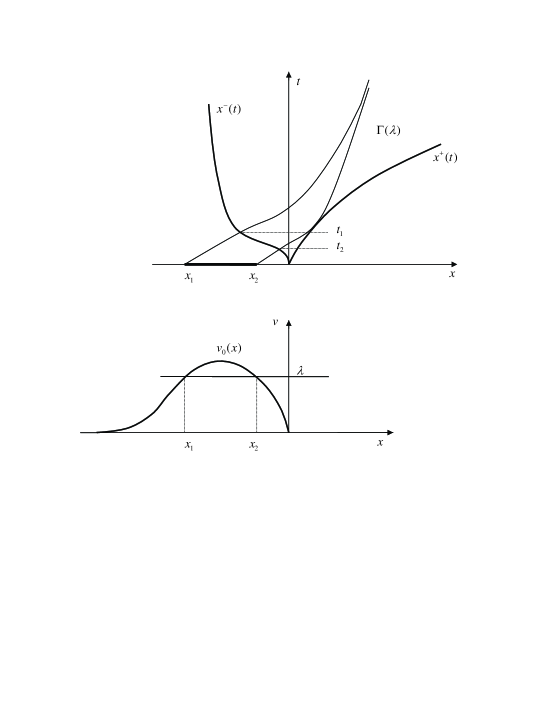
Figure 1: $\lambda$-section of the initial profile (below) and the behaviour of the corresponding confining characteristics for part of the KdV modulation solution (above). $\Gamma(\lambda)$ is the domain of influence of the interval $[x_{1},x_{2}]$

To clarify the meaning of the quantity $F(\lambda)$ in the framework of modulation theory we introduce the notion of a $\lambda$-section of the initial profile, which is simply a segment of the function $v_{0}(x)$ for which $v_{0}(x)\geq\lambda$ (see Fig. 1), and consider the integral

$$F(\lambda,t)=\frac{1}{2\pi}\int_{x_{1}+\lambda t}^{x_{2}+\lambda t}\sqrt{(2/3)(\overline{v}(x,t)-\lambda)}dx$$ (46)

for $t<t_{2}$, where $t_{2}$ is the time at which the characteristic $x=x_{2}+\lambda t$ intersects the trailing edge $x^{-}(t)$ of the undular bore $x^{-}(t_{2})=x_{2}+\lambda t_{2}$ (see Fig. 1). Note that this $t_{2}$ plays for the $\lambda$-section of the (evolving) profile $v(x,t)$ a role similar to the breaking time, as the nonlinear oscillations emerge in the vicinity of the point $(x^{-}(t_{2}),t_{2})$ and the system (22) ceases to be valid. However, unlike at the breaking point, there is no gradient catastrophe at $(x^{-}(t_{2}),t_{2})$.

We now see that for $t<t_{2}$ one has $\partial F/\partial t=0$ and thus $F(\lambda,t)=F(\lambda,0)=F(\lambda)$. Indeed the integrand in (46) is nothing but the exact solution (24) of the modulation system (22). But this system conserves the integral $\int_{-\infty}^{+\infty}k(\overline{v}(x,t))dx$, so that we have

$$\frac{1}{2\pi}\int_{-\infty}^{+\infty}k(\overline{v}(x,t))dx=\frac{1}{2\pi}\int_{x_{1}+\lambda t}^{x_{2}+\lambda t}k(\overline{v}(x,t))dx=\frac{1}{2\pi}\int_{x_{1}}^{x_{2}}k(v_{0}(x))dx=F(\lambda)\,.$$ (47)

It follows from (47) that $F(\lambda)$ is the number of linear modulated waves (i.e. the number of wave crests) “contained” in the $\lambda$-section of the initial profile. All these waves are “released” into the undular bore during the time interval $(t_{2},t_{1})$ (see Fig. 1) and eventually transform into solitons as $t\to\infty$.

Now we establish a correspondence between the $\lambda$-section of the initial profile and a certain part of the solitary wavetrain as $t\to\infty$. This correspondence follows from the detailed consideration of the behaviour of the characteristics for the modulation solution made in Gurevich, Krylov & Mazur [30] where it was shown that all the characteristics of the modulation system issuing from the points of the interval $[x_{1},x_{2}]$ are confined to the area $\Gamma(\lambda)$ of $(x,t)$-plane enclosed by the leading edge $x^{+}(t)$ and the characteristic emerging from $x_{1}$ (see Fig. 1). On the other hand, it was shown that for sufficiently large $t$ the characteristics emerging from the points $x\notin[x_{1},x_{2}]$ lie entirely outside $\Gamma(\lambda)$. Therefore all wave crests generated at the trailing edge between the points $x^{-}_{2}=x_{2}+\lambda t_{2}$ and $x^{-}_{1}=x_{1}+\lambda t_{1}$ remain within the described region $\Gamma(\lambda)$ for all $t$ and eventually transform into the portion of solitons having their amplitudes in the interval $[a(\lambda);a(A)]$. In other words, $\Gamma(\lambda)$ represents the domain of influence of the interval $[x_{1},x_{2}]$ and thus, formula (45) defines the number of solitons in this region as $t\to\infty$. Indeed when $\lambda=0$ it coincides with formula (43) for the total number of solitons.

We still need to find the dependence $a(\lambda)$ to obtain the distribution of solitons as a function of amplitude. In this regard we take advantage of the fact that due to the condition $v(x,0)=0$ for $x>0$, all solitons propagate on a zero background, so substituting $\overline{v}=0$ into $I_{2}$ we obtain $\lambda=3\widetilde{k}^{2}/2$. Now using the connection (30) between the inverse width of a KdV soliton and its amplitude we obtain the relationship $a=2\lambda$. In particular we immediately recover the IST formula $a_{max}=a(A)=2A$ (see (9)). Then differentiating $F(\lambda)$ with respect to $a$ we obtain Karpman’s formula (11) for the soliton amplitude distribution function

$$f(a)=\left|\frac{dF(a/2)}{da}\right|=\frac{1}{4\pi}\frac{1}{\sqrt{6}}\int_{x_{1}}^{x_{2}}\frac{dx}{\sqrt{v_{0}(x)-a/2}}\,.$$ (48)

Summarising, we have managed to reproduce the semi-classical IST results pertaining to soliton dynamics using, technically, only the linear dispersion relation and the characteristic velocity of the KdV equation in the dispersionless limit. Of course, we took advantage of our knowledge of the qualitative behaviour of the characteristics of the modulation equations for the solutions considered here. Next assuming the same qualitative behaviour of modulations as a plausible assumption, we extend the above reasoning to the non-integrable SG model (1) with the aim of obtaining the counterparts of the formulae (43) and (48) for fully nonlinear shallow water dynamics. Our analytic results will then be compared with full numerical solutions of the SG system.

3 Asymptotic description of a solitary wavetrain in the Su-Gardner system

3.1 Conserved quantities in the SG solitary wavetrain

We consider the SG system (1) with the initial depth profile

$$\eta(x,0)=\eta_{0}(x)>1\,:\ \ \eta_{0}(x)\to 1\quad\text{as}\quad|x|\to\infty$$ (49)

and the velocity profile connected with (50) by the simple wave relationship

$$u(x,0)=u_{0}(x)=2(\sqrt{\eta_{0}(x)}-1)\,,$$ (50)

so that $u_{0}(x)\to 0$ as $|x|\to\infty$. Let $\max[\eta_{0}(x)]=1+A$ and let $w$ be the typical width of $\eta_{0}(x)$. Similarly to the KdV case we shall assume that $A^{1/2}w\gg 1$. Also, for convenience, we assume that $\eta_{0}(x)=1$ for $x>0$, which will guarantee that solitary waves propagate on the undisturbed background $\eta=1$.

Figure 2: Solitary wavetrain developing in the SG system from the initial disturbance (55) with $A=1$ and $w=10$. The plot is $\eta(x,t)$ at $t=400$.

The system (1) conserves the four physical quantities

$$J_{1}=\int[\eta-1]dx;\qquad\hbox{mass}$$ (51)

$$J_{2}=\int[u+\frac{1}{6}\eta^{2}u_{xx}]dx;\qquad\hbox{irrotationality}$$ (52)

$$J_{3}=\int[\eta u]dx;\qquad\hbox{momentum}$$ (53)

$$J_{4}=\int[\frac{1}{2}(\eta-1)^{2}+\frac{1}{2}\eta u^{2}+\frac{1}{6}\eta^{3}u_{x}^{2}]dx\qquad\hbox{energy}.$$ (54)

We now consider the SG system with the specific initial conditions

$$\eta_{0}(x)=1+A\ \hbox{sech}^{2}[x/w],\qquad u_{0}(x)=2(\sqrt{\eta_{0}(x)}-1)\,$$ (55)

with the aim of verifying numerically some of our main assumptions about the qualitative features of the asymptotic behaviour as $t\to\infty$. A typical long-time outcome is shown in Fig. 2. Comparison of the values of the four conserved quantities (51)–(54) computed for two initial profiles having the form (55) with $A=0.4$, $w=13$ and $A=2$, $w=10$ with their values calculated for the solitary wavetrain at large $t$ shows that the relative change, due to radiation, is $O(10^{-2})$, which is within the accuracy of modulation theory, valid for $\epsilon=(A^{1/2}w)^{-1}=0.12$ and $0.07$ respectively. Therefore we can assume that with good accuracy a positive large-scale initial disturbance is completely transformed as $t\to\infty$ into a solitary wavetrain and we can neglect the contribution of the radiation component in the modulation analysis.

3.2 Modulation characteristic integrals

We now apply the procedure for the derivation of the amplitude distribution function, developed in Section 2 in the context of the KdV equation, to the SG system. The key objects are the modulation characteristic integrals, having in the KdV case the form (37) and (38). The ordinary differential equations for these integrals for the SG case (the counterparts of the KdV case equations (23) and (35)) were derived in El, Grimshaw & Smyth [10], so here we present only the resulting formulae. It is important to mention that the derivation in El, Grimshaw & Smyth [10] was performed in the context of simple undular bores, so that it incorporated the simple wave relationships between the depth and velocity jumps across the bore. In the present study this condition is automatically satisfied by choosing initial conditions in the form (49) and (50).

The key ingredient of the modulation characteristic integrals is the linear dispersion relation for modulations, which in the SG case has the form

$$a=0:\qquad\omega=\omega_{0}(\bar{\eta},\bar{u},k)=k\left(\bar{u}+\frac{\bar{\eta}^{1/2}}{(1+\bar{\eta}^{2}k^{2}/3)^{1/2}}\right)\,.$$ (56)

Here, as for $\overline{v}$ in (15), $\overline{\eta}$ and $\overline{u}$ denote the values averaged over the period of the travelling wave. Next we incorporate the simple wave relation $\overline{u}(\overline{\eta})=2(\sqrt{\overline{\eta}}-1)$ into (56) to obtain the dispersion relation for a linear dispersive wave propagating on a slowly varying simple wave background

$$\Omega_{0}(\overline{\eta},k)=\omega_{0}(\overline{\eta},\overline{u}(\overline{\eta}),k)=2k(\overline{\eta}^{1/2}-1)+\frac{k\overline{\eta}^{1/2}}{(1+\overline{\eta}^{2}k^{2}/3)^{1/2}}\,.$$ (57)

Next, using reasoning identical to that described in Section 2 (see [10, 26, 28] for additional details pertaining to bidirectional systems), we obtain the characteristic integrals of the modulation system defined by the ordinary differential equations

$$I_{1}:\qquad a=0,\quad\frac{dk}{d\overline{\eta}}=\frac{\partial\Omega_{0}/\partial\overline{\eta}}{V(\overline{\eta})-\partial\Omega_{0}/\partial k}\quad\hbox{on}\quad\frac{dx}{dt}=\frac{\partial\Omega_{0}}{\partial k}\,,$$ (58)

$$I_{2}:\qquad k=0\,,\quad\frac{d\widetilde{k}}{d\overline{\eta}}=\frac{\partial\widetilde{\Omega}_{0}/\partial\overline{\eta}}{V(\overline{\eta})-\partial\widetilde{\Omega}_{0}/\partial\widetilde{k}}\quad\hbox{on}\quad\frac{dx}{dt}=\frac{\widetilde{\Omega}_{0}}{\widetilde{k}}\,.$$ (59)

Here

$$V(\overline{\eta})=\overline{u}(\overline{\eta})+\overline{\eta}^{1/2}=3\overline{\eta}^{1/2}-2$$ (60)

is the characteristic velocity of the right-propagating simple wave of the ideal shallow water equations (i.e. the dispersionless limit of the SG system) and

$$\widetilde{\Omega}_{0}(\overline{\eta},\widetilde{k})=-i\Omega_{0}(\overline{\eta},i\widetilde{k})=2\widetilde{k}(\overline{\eta}^{1/2}-1)-\frac{\widetilde{k}\overline{\eta}^{1/2}}{(1-\overline{\eta}^{2}\widetilde{k}^{2}/3)^{1/2}}\,$$ (61)

is the SG “solitary wave dispersion relation”, an analogue of the KdV formula (29), $\widetilde{k}$ being the soliton wavenumber.

Substituting (57) into (58) and introducing $\alpha=(1+k^{2}\overline{\eta}^{2}/3)^{-1/2}$ as a new variable instead of $k$ we obtain an ordinary differential equation in separated form

$$\frac{d\overline{\eta}}{\overline{\eta}}=\frac{2(1+\alpha+\alpha^{2})}{\alpha(1+\alpha)(\alpha-4)}d\alpha\,\,.$$ (62)

Integrating (62) we obtain

$$\frac{\overline{\eta}}{\lambda_{1}}=\frac{1}{{\alpha}^{1/2}}\left(\frac{4-\alpha}{3}\right)^{21/10}\left(\frac{1+\alpha}{2}\right)^{2/5}\,,$$ (63)

where $\lambda_{1}$ is an arbitrary constant of integration. Similarly, substituting (61) into (59) and then using $\widetilde{\alpha}=(1-{\widetilde{k}}^{2}\overline{\eta}^{2}/3)^{-1/2}$ instead of $\widetilde{k}$ we arrive at the same separated ordinary differential equation (62), but now for for $\widetilde{\alpha}(\overline{\eta})$

$$\frac{d\overline{\eta}}{\overline{\eta}}=\frac{2(1+\widetilde{\alpha}+\widetilde{\alpha}^{2})}{\widetilde{\alpha}(1+\widetilde{\alpha})(\widetilde{\alpha}-4)}d\widetilde{\alpha}$$ (64)

with the integral

$$\frac{\overline{\eta}}{\lambda_{2}}=\frac{1}{{\widetilde{\alpha}}^{1/2}}\left(\frac{4-\widetilde{\alpha}}{3}\right)^{21/10}\left(\frac{1+\widetilde{\alpha}}{2}\right)^{2/5}\,,$$ (65)

$\lambda_{2}$ being another constant of integration.

Now we recall that the constants $\lambda_{1}$ and $\lambda_{2}$ cannot be set independently if the characteristic integrals (63) and (65) are considered in the context of the same modulation solution. One can see from the zero amplitude integral $I_{2}$ (63) that $\overline{\eta}=\lambda_{1}$ implies $\alpha=1$ and, therefore, $k=0$. But $k=0$, in its turn, corresponds to the solitary wave limit, so the equality $\overline{\eta}=\lambda_{1}$ must be consistent with the zero amplitude reduction of the “soliton” integral $I_{2}$ (65). To obtain this reduction we calculate the solitary wave velocity using the conjugate dispersion relation (61)

$$c=\frac{\widetilde{\Omega}_{0}(\overline{\eta},\widetilde{k})}{\widetilde{k}}=2(\overline{\eta}^{1/2}-1)-\overline{\eta}^{1/2}\widetilde{\alpha}\,.$$ (66)

On the other hand, we have from (3), after replacing $\eta_{0}$ with $\overline{\eta}$ and $u_{0}$ with $\overline{u}=2(\overline{\eta}^{1/2}-1)$,

$$c=2(\overline{\eta}^{1/2}-1)+\sqrt{\overline{\eta}+a}\,.$$ (67)

Comparing (66) and (67) we obtain the expression for the solitary wave amplitude in terms of the variable $\widetilde{\alpha}$, an analogue of the KdV formula (30),

$$k=0:\qquad a=\overline{\eta}(\widetilde{\alpha}^{2}-1)\,.$$ (68)

Now one can see that the reduction as $k=0$, $a=0$ implies $\widetilde{\alpha}=1$ which, by (65), immediately yields $\overline{\eta}=\lambda_{2}$. Therefore, similar to the KdV case, we have $\lambda_{1}=\lambda_{2}\equiv\lambda$ and the relationships (63) and (65) become a set of two consistent modulation characteristic integrals parametrised by the same value $\lambda$ (cf. (37) and (38) for the KdV case).

3.3 Total number of solitary waves

As we described in Section 2.2 the total number of solitary waves in the soliton train evolving out of the initial large-scale disturbance (49) and (50) can be found from the modulation formula

$$N\cong\frac{1}{2\pi}\int_{-\infty}^{+\infty}k_{0}(x)dx\,,$$ (69)

where $k_{0}(x)$ is the initial distribution of the wavenumber corresponding to the initial conditions (49) and (50) for the depth $\eta$ and velocity $u$. This distribution is found from the group velocity characteristic integral of the zero amplitude reduction of the modulation equations. In the case of the SG system this is the integral $I_{1}$ given by formula (63), in which one assumes $\lambda_{1}=\lambda=1$. The latter equality follows from the requirement that the integral $I_{1}$ must correctly reproduce the mean value $\overline{\eta}=1$ for the solitary wave background when one sets $k=0$ (i.e. $\alpha=1$) in (63). Next one replaces $\overline{\eta}$ in $I_{1}$ with its distribution $\eta_{0}(x)$ at $t=0$ to obtain an implicit expression for $k_{0}(x)$ in terms of $\eta_{0}(x)$

$$\eta_{0}(x)=\frac{1}{\sqrt{\alpha_{0}}}\left(\frac{4-\alpha_{0}}{3}\right)^{21/10}\left(\frac{1+\alpha_{0}}{2}\right)^{2/5}\,,$$ (70)

where $\alpha_{0}(x)$ is connected with $k_{0}(x)$ via the relationship

$$\alpha_{0}=(1+(k_{0}\eta_{0}(x))^{2}/3)^{-1/2}\,.$$ (71)

Thus expressing $k_{0}$ from (71) and substituting it into (69) we obtain

$$N\cong\frac{1}{2\pi}\int_{-\infty}^{+\infty}\frac{\sqrt{3(1-\alpha_{0}^{2}(x))}}{\eta_{0}(x)\alpha_{0}(x)}dx\,,$$ (72)

which, together with (70), completely defines the total number of solitary waves forming in the initial value problem (1), (49) and (50).

    

Figure 3: Total number of solitary waves forming due to the decay of the initial disturbance (55). The initial parameters are $w=10$ and $A$ varying (left); $A=0.4$ and $w$ varying (right). Solid line is the modulation formula (72); symbols are the numerical solution; the dashed line is the formula (73) corresponding to the KdV approximation (4).

The first term of the expansion of (72) and (70) in $\eta_{0}(x)-1\ll 1$ (i.e.  $1-\alpha_{0}\ll 1$ by (70)) yields

$$N\sim\sqrt{\frac{3}{2}}\frac{1}{\pi}\int_{-\infty}^{+\infty}\sqrt{\eta_{0}(x)-1}dx\,,$$ (73)

corresponding to the KdV result (43), taking into account that the weakly nonlinear reduction of the SG system yields the KdV equation in the form (5), so to obtain (43) one needs firstly to set $\eta_{0}(x)-1=\zeta_{0}(x)$ in (73) and then apply the rescaling as described in Section 1.

To compare our analytical results with full numerical solutions of the SG system we consider the dependence of $N$ on $A^{1/2}w$, which is the parameter suggested by dimensional analysis (see also (12)), for initial data of the form (55). The results are shown in Fig. 3. The comparison shown in the left panel is for the solitary wavetrain developing from the initial profile (55), with the width set to $w=10$ and the amplitude $A$ varying so that $A^{1/2}w$ varies in the interval $[6,13]$, while in the right panel we fix the amplitude to $A=0.4$ and vary the width $w$ so that the quantity $A^{1/2}w$ has the same range $[6,13]$. One can see that in both cases the modulation formula predicts the total number of solitary waves very well. The over-prediction by just one in the second comparison is clearly within the accuracy of the modulation approach, which is $O(A^{1/2}w)^{-1})$.

3.4 Amplitude distribution function

Next, following the procedure of Section 2.3, we can “upgrade” formula (72) by using in (69) the full expression $k_{0}(x,\lambda)$, which is obtained from the modulation characteristic integral $I_{1}$ (63) by retaining the parameter $\lambda$ and replacing the mean depth $\overline{\eta}$ with its initial distribution $\eta_{0}(x)$. The expected result is the SG analogue of the integrated KdV soliton amplitude distribution function (45).

We thus assume that in (71) $\alpha_{0}=\alpha_{0}(x,\lambda)$ and then obtain from (63) an implicit expression

$$\frac{\eta_{0}(x)}{\lambda}=\frac{1}{\sqrt{\alpha_{0}}}\left(\frac{4-\alpha_{0}}{3}\right)^{21/10}\left(\frac{1+\alpha_{0}}{2}\right)^{2/5}\,.$$ (74)

Then the integrated distribution function has the form

$$F(\lambda)\cong\frac{1}{2\pi}\int^{x_{2}}_{x_{1}}k_{0}(x,\lambda)dx\,,$$ (75)

where the function $k_{0}(x,\lambda)$ is expressed in terms of $\alpha_{0}(x,\lambda)$ as

$$k_{0}(x,\lambda)=\frac{\sqrt{3(1-\alpha^{2}(x,\lambda))}}{\eta_{0}(x)\alpha(x,\lambda)}\,$$ (76)

(see(71)) and $x_{1,2}(\lambda)$ are the roots of the equation $k_{0}(x,\lambda)=0$. It immediately follows from (76) and (74) that these roots coincide with the roots of $\eta_{0}(x)=\lambda$. So the range of $\lambda$ is $[1,1+A]$, where $A=\max[\eta_{0}(x)]-1$.

Figure 4: Comparison of the lead solitary wave amplitude $a_{m}$ as a function of the initial amplitude $A$. The initial conditions are (55) with $w=15$. Solid line is the analytical solution (78), the dashed line is the numerical solution.

Next we establish the connection between the parameter $\lambda$ and the lower bound of the amplitude range in the portion of solitary waves corresponding to the “$\lambda$-section” of the initial profile $\eta_{0}(x)$. This is found from the characteristic integral $I_{2}$ (65), in which we set $\lambda_{2}=\lambda$ and $\overline{\eta}=1$ as here the solitary waves are on a unit background (recall that $\eta_{0}(x)=1$ for $x>0$). Then substituting $\widetilde{\alpha}=\sqrt{1+a}$ from (68) we obtain the required relationship

$$\lambda=(1+a)^{1/4}\left(\frac{3}{4-\sqrt{1+a}}\right)^{21/10}\left(\frac{2}{1+\sqrt{1+a}}\right)^{2/5}\,.$$ (77)

      

Figure 5: Number $\mathcal{N}(a)$ of solitary waves with amplitudes in the interval $[a,a_{m}]$ generated from the initial conditions (55) with $A=0.4$, $w=13$ (left) and $A=2$, $w=10$ (right). Solid line is the modulation formula (75); symbols are the numerical solution; dashed line is the integrated Karpman formula (79).

Since $\max\lambda=1+A$, the amplitude of the largest solitary wave $a_{m}$ is found from the equation

$$1+A=(1+a_{m})^{1/4}\left(\frac{3}{4-\sqrt{1+a_{m}}}\right)^{21/10}\left(\frac{2}{1+\sqrt{1+a_{m}}}\right)^{2/5}\,.$$ (78)

Expanding (78) in $a_{m}$ we obtain to leading order $a_{m}=2A$, as expected from weakly nonlinear KdV theory. The relation (78) is shown in Fig. 4 along with the amplitude curve obtained from direct numerical solutions of the SG system (1) with the initial conditions (55) with $w=15$. One can see that the agreement is very good for solitary wave amplitudes up to about $a=1.6$. The departure of the analytical curve from the numerical one for larger amplitudes will be discussed later. One can also observe that the KdV lead soliton amplitude curve $a_{m}=2A$ gives a very good approximation to the numerical SG curve, in fact even better than the modulation SG formula (78). One should, however, bear in mind that formula (78) for the lead solitary wave amplitude should be used in conjunction with expressions (2) and (3) defining the SG solitary wave profile and velocity and, as such, then provides a consistent approximation of the SG solution (and therefore of the full Euler equations solution). At the same time the KdV formula $a_{m}=2A$ should be considered together with the familiar KdV soliton profile and the speed-amplitude dependence (16) which are known not to give very good approximations to the SG solitary wave for large amplitudes.

Figure 6: Amplitude profile of the SG solitary wavetrain at $t=1500$. The parameters of the initial profile are $A=2$ and $w=10$. Solid line is the formula (81); symbols are the numerical solution; dotted line is the KdV soliton train amplitude profile (83)

Next putting (75)–(77) together we obtain the formula for the number of solitary waves with amplitudes in the interval $[a,a_{m}]$ as $\mathcal{N}(a)=F(\lambda(a))$. Indeed $\mathcal{N}(0)=F(1)=N$, where $N$ is the total number (72) of solitary waves in the train. Expanding (75)–(77) in $a$ for $a\ll 1$ we obtain to leading order

$$\mathcal{N}(a)\sim\sqrt{\frac{3}{2}}\frac{1}{\pi}\int_{x_{1}}^{x_{2}}\sqrt{(\eta_{0}(x)-1)-a/2}\ dx,$$ (79)

where $x_{1,2}(a)$ are the roots of the equation $\eta_{0}(x)=1+a/2$. Equation (79) is the integrated Karpman formula for the KdV equation in the form (4) (cf. (45)). Comparisons of the integrated amplitude distribution function $\mathcal{N}(a)$ with the numerically found number of solitons are shown in Fig. 5 for two different initial profiles (one with $A=0.4$, $w=13$ (left panel) and another one with $A=2$, $w=10$ (right panel)). One can see that the agreement in both cases is quite good (again taking into account the accuracy of the modulation approach itself). Moreover, one can see from the comparison in the right panel that the modulation formula appears to work reasonably well far beyond the range of formal applicability of the GP formulation of the problem used here. Indeed, it was shown in El, Grimshaw and Smyth [10] that starting from some critical depth jump $\Delta_{cr}\approx 1.4$ across the SG undular bore, the oscillatory structure of the bore qualitatively changes due to linear degeneration of the characteristic field and formation of a rapidly varying, finite amplitude rear wavefront, as opposed to the usual vanishing amplitude trailing wave packet assumed in the GP formulation. As an estimate we can assume $A/2=\Delta-1$, the value of an “effective jump” taken at the level of half the maximum value of the depth disturbance. Then for solitary waves with amplitudes greater than $a_{cr}\approx 0.8$ one can expect some discrepancy between the modulation predictions and the results of direct numerical simulations, as indeed seen in Fig. 4.

The solitary wave density distribution function $f(a)$ is obtained by differentiating (79)

$$f(a)=\frac{d\mathcal{N}}{da}\,,$$ (80)

so that $f(a)da$ gives the number of solitons with amplitudes in the interval $[a,a+da]$. If we let the number of solitary waves per unit length in the solitary wavetrain be $\kappa$, then it follows from the balance relationship $\kappa dx=f(a)da$ that $\kappa=f(a)da/dx$. Since the speed of an SG solitary wave propagating against a background $\eta=1$ and $u=0$ is $c=\sqrt{1+a}$, the amplitude profile in the solitary wavetrain for $x,t\gg 1$ is found from the general formula $\sqrt{1+a}=x/t+\mathcal{O}(t^{-1})$ as

$$a\cong(x/t)^{2}-1\,.$$ (81)

A comparison of formula (81) for the solitary wavetrain amplitude profile with the numerical profile for $A=2$ and $w=10$ at $t=1500$ is shown in Fig. 6

      

Figure 7: Spatial density of solitary waves $\kappa(x,t)$ in the solitary wavetrain formed out of the initial profile (55) with $A=0.4$, $w=13$ (left, $t=1400$) and $A=2$, $w=10$ (right, $t=1500$). Solid line is the SG formula (82); symbols are the numerical solution; dotted line is the KdV formula(83).

Next, for the number of solitons per unit length we obtain

$$\kappa\cong\frac{2x}{t^{2}}f(({x}/{t})^{2}-1)\,.$$ (82)

We note that the weakly nonlinear counterparts of formulae (81) and (82) corresponding to the KdV equation in the form (4) are

$$a\cong 2({x}/{t}-1)\,,\qquad\kappa\cong\frac{2}{t}f_{KdV}(2(x/t-1))\,,$$ (83)

where $f_{KdV}(a)$ is given by the Karpman formula (11). Comparisons of the curve (82) with the numerically found spatial density of solitary waves in the SG solitary wavetrain for two different initial profiles are shown in Fig. 7. As in the previous comparisons, the agreement is excellent for moderate ($A=0.4$) and reasonably good for very large ($A=2$) amplitudes of the initial disturbance (55).

4 Conclusions

We have developed a general method for obtaining an asymptotic description of solitary wavetrains for initial value problems for weakly dispersive nonlinear systems which may not be integrable via the IST. The method is based on the properties of the characteristics of the associated modulation (Whitham) system describing an intermediate undular bore stage of the evolution. We have demonstrated the effectiveness of the developed approach by firstly recovering the semi-classical IST results for the soliton amplitude distribution function for the KdV equation and then by applying it to the Su-Gardner (SG) system (1), the 1D version of the Green-Naghdi equations, describing fully nonlinear shallow water waves. The SG system is not integrable by the IST, but has enough structure (a periodic travelling wave solution family and four conservation laws) to be amenable to a nonlinear modulation analysis. It also transpires that the SG system represents an important mathematical model for understanding general properties of fully nonlinear fluid flows beyond the strict shallow water limit. For this reason we have studied its solutions for the full range of amplitudes, although in the particular context of shallow water waves the system (1) is unable to reproduce the effects of wave overturning and becomes nonphysical for amplitudes greater than some critical value.

The resulting asymptotic formulae for the solitary wave amplitude distribution function, the total number of solitary waves and the amplitude of the leading solitary wave in the solitary wavetrain formed as the long time outcome of the decay of an initial large scale, one hump depth disturbance have been compared with the results of direct numerical simulations of the Su-Gardner system. Very good agreement between the modulation solution and numerical results have been demonstrated, even for the range of initial amplitudes significantly exceeding that for the applicability of modulation theory due to formation of a rapidly varying wavefront at the trailing edge of the undular bore at an intermediate stage of its evolution (see El, Grimshaw and Smyth [10]).

The results obtained for fully nonlinear shallow water theory have also been compared with their weakly nonlinear counterparts which are well known from the semi-classical IST approach to the KdV equation, where they were obtained as consequences of the famous Bohr-Sommerfeld quantisation rule (see Whitham [14] and Karpman [15]). Overall, one can conclude that KdV theory gives a very good prediction for the lead solitary wave amplitude and the spatial density of solitary waves in the fully nonlinear solitary wavetrain, but consistently over-predicts the number of solitary waves in a given amplitude interval. Indeed this discrepancy grows with the initial amplitude. One can also note that this comparison is consistent with the modulation results for SG undular bores in the step resolution problem studied in El, Grimshaw and Smyth [10], where it was shown that the SG undular bore is noticeably narrower and contains less wavecrests than its KdV counterpart for moderate to large values of the depth jump across the bore. Also, due to the essentially different amplitude-speed relationships for SG and KdV solitary waves (cf. (3) and (16), the former being actually equivalent to that for the full Euler theory [11]), the spatial amplitude profile of the SG solitary wavetrain is parabolic, in contrast to the KdV classical triangle profile (see Whitham [14] and Fig. 6).

Acknowledgements

The authors thank A. Kamchatnov for useful discussions.

References

- [1] A.E. Green and P.M. Naghdi, “A derivation of equations for wave propagation in water of variable depth,” J. Fluid Mech., 78, 237 (1976).
- [2] S.L. Gavrilyuk, “Large amplitude oscillations and their “thermodynamics” for continua with “memory”,” Eur. J. Mech., B/Fluids, 13, 753 (1994).
- [3] P.J. Dellar, “Dispersive shallow water magnetohydrodynamics,” Physics of Plasmas, 10, 581 (2003).
- [4] S.L. Gavrilyuk and V.M. Teshukov, “Generalized vorticity for bubbly liquid and dispersive shallow water equations,” Continuum Mech. Thermodyn., 13, 365 (2001).
- [5] C.H. Borzi, R.A. Kraenkel, M.A. Manna and A. Pereira, “Nonlinear dynamics of short travelling capillary-gravity waves,” Phys. Rev. E, 71, 026307 (2005).
- [6] W. Choi and R. Camassa, “Fully nonlinear internal waves in a two-fluid system,” J. Fluid Mech., 396, 1 (1999).
- [7] L.A. Ostrovsky and J. Grue, “Evolution equations for strongly nonlinear internal waves,” Phys. Fluids, 15, 2934 (2003).
- [8] R. Barros, S. L. Gavrilyuk and V. M. Teshukov, “Dispersive Nonlinear Waves in Two-Layer Flows with Free Surface. I. Model Derivation and General Properties,” Stud. Appl. Math., 119, 191–211 (2007).
- [9] C.H. Su and C.S. Gardner, “Korteweg-de Vries equation and generalisations III. Derivation of the Kortwewg-de Vries equation and Burgers equation,” J. Math. Phys., 10, 536 (1969).
- [10] G. El, R.H.J. Grimshaw and N.F. Smyth, “Unsteady undular bores in fully nonlinear shallow-water theory,” Physics of Fluids, 18, 027104 (2006).
- [11] Lord Rayleigh, “On Waves,” Phil. Mag., 1, 257 (1876).
- [12] R.S. Johnson, “Camassa-Holm, Korteweg-de Vries and related models for water waves,” J. Fluid Mech., 455, 63 (2002).
- [13] V.I. Karpman, “An asymptotic solution of the Korteweg-de Vries equation,” Phys. Lett. A, 25, 708–709 (1967).
- [14] G.B. Whitham, Linear and Nonlinear Waves, (Wiley, New York, 1974).
- [15] V.I. Karpman, Nonlinear Waves in Dispersive Media, (Pergamon, Oxford, 1975).
- [16] A.M. Kamchatnov, R.A. Kraenkel and B.A. Umarov, Phys. Rev. E, 66, 036609 (2002).
- [17] A.M. Kamchatnov, R.A. Kraenkel and B.A. Umarov, “Asymptotic soliton train solutions of Kaup-Boussinesq equations,” Wave Motion, 38, 355–365 (2003).
- [18] P.D. Lax, C.D. Levermore and S. Venakides, “The generation and propagation of oscillations in dispersive initial value problems and their limiting behavior,” in Important developments in soliton theory, ed. by A.S. Fokas and V.E. Zakharov, (Springer Ser. Nonlinear Dynam., Springer, Berlin 1994) p. 205 (1994).
- [19] G.B. Whitham, “Non-linear dispersive waves,” Proc. Roy. Soc. London, 283A, 238 (1965).
- [20] J.C. Luke, “A perturbation method for nonlinear dispersive wave problems,” Proc. Roy. Soc. Lond., A292 (1966).
- [21] S. Yu. Dobrokhotov and V.P. Maslov, “Multiphase asymptotics of nonlinear partial differential equations with a small parameter,” Sov. Sci. Rev.: Math. Phys., 3, 221–280 (1982).
- [22] A.V. Gurevich, A.L. Krylov, N.G. Mazur N.G. and G.A. El, “Evolution of a localized perturbation in Korteweg-de Vries hydrodynamics,” Sov. Phys. Doklady, 37, 198–201 (1992).
- [23] G. El and R.H.J Grimshaw, “Generation of undular bores in the shelves of slowly-varying solitary waves,” Chaos, 12, 1015–1026 (2002).
- [24] H. Flaschka, G. Forest & D.W. McLaughlin, “Multiphase averaging and the inverse spectral solutions of the Korteweg-de Vries equation,” Comm. Pure Appl. Math., 33, 739–784 (1979).
- [25] R. Courant and D. Hilbert, Methods of Mathematical Physics, Vol II, Wiley-Interscience, New York, (1962).
- [26] G.A. El, “Resolution of a shock in hyperbolic systems modified by weak dispersion,” Chaos, 15, 037103 (2005).
- [27] A.V. Gurevich and L.P. Pitaevskii, “Nonstationary structure of a collisionless shock wave,” Sov. Phys. JETP, 38, 291 (1974).
- [28] G.A. El, V.V. Khodorovskii, and A.V. Tyurina, “Undular bore transition in bi-directional conservative wave dynamics,” Physica D, 206, 232 (2005).
- [29] R.H.J. Grimshaw, “Slowly varying solitary waves. I Korteweg-de Vries equation,” Proc. Roy. Soc. Lond., 368A, 359–375 (1979).
- [30] A.V. Gurevich, A.L. Krylov and N.G. Mazur, “Quasismple waves in Korteweg-de Vries hydrodynamics,” Sov. Phys. JETP, 68, 966–974 (1989).
- [31] G.A. El, V.V. Khodorovskii, and A.V. Tyurina, “Determination of boundaries of unsteady oscillatory zone in asymptotic solutions of non-integrable dispersive wave equations,” Phys. Lett. A, 318, 526 (2003).
- [32] G.A. El, R.H.J. Grimshaw and M.V. Pavlov, “Integrable shallow-water equations and undular bores,” Stud. Appl. Math., 106, 157 (2001).
- [33] R.H.J. Grimshaw and N.F. Smyth, “Resonant flow of a stratified fluid over topography,” J. Fluid Mech., 169, 429–464 (1986).
- [34] A.M. Kamchatnov, Nonlinear Periodic Waves and Their Modulations—An Introductory Course, (World Scientific, Singapore, 2000)
- [35] L.D. Landau and E.M. Lifshitz, Fluid Mechanics, (Pergamon, Oxford, 1987).
- [36] N.F. Smyth, “Modulation theory for resonant flow over topography,” Proc. Roy. Soc. Lond., A409, 79–97 (1987).