Applications of Level Curves to Some Problems on Algebraic Surfaces

Abstract

In JGRS , a result to algorithmically compute the topology types of the level curves of an algebraic surface, is given. From this result, here we derive applications based on level curves to determine some topological features of surfaces (reality, compactness, connectivity) and to the problem of plotting.

,

1 Introduction

The study of the level curves of an implicit algebraic surface (i.e. the sections of the surface with real planes parallel to the $xy$-plane) gives a clue on how the surface is like. Take for example the well-known example of the Whitney Umbrella, whose equation is $x^{2}-y^{2}z=0$. It is clear that for $z>0$ the level curves consist of two intersecting lines; for $z=0$, the level curve reduces to one line; and for $z<0$, the level curves consist of just one real isolated point. From this simple analysis one may get a good mental picture of the surface. Moreover, it provides an initial analysis to the topology of the surface, which can be used later to provide topologically-correct plottings. For instance, in the case of the Whitney Umbrella one has that a topologically-correct plotting must show the so-called “handle” of the surface, i.e. the half-line corresponding to $x=0,y=0,z\leq 0$. Moreover, in addition to the shape of the level curves, one also has the $z$-intervals corresponding to each topology type.

The problem of computing the different topology types arising in the family of level curves of a given algebraic surface (together with the $z$-values corresponding to each type) has been addressed, for instance in JGRS and Mourrain-2 , where algorithms to compute these topology types are given. Moreover, in JGRS applications of this approach to the study of offset curves are also given; see also JG-Sendra07 for further research on this topic. Now, in this paper, we apply these results on level curves to determine topological information on the surface, which may be of help for computing reliable plottings from the topological point of view.

In this sense, the first application that we consider is to algorithmically decide whether a given implicit algebraic surface is real. That is, we provide an algorithm to check whether the intersection of the surface with ${\mathbb{R}}^{3}$ is a two-dimensional set (in the Euclidean topology) or not. Furthermore, in the negative case, the algorithm can also be used to analyze whether the real part of the surface is empty (like for example $x^{2}+y^{2}+z^{2}+1=0$), or it consists of finitely many points (the case of $x^{2}+y^{2}+z^{2}=0$, whose real part is the origin) or it is a space curve (the case of $x^{2}+y^{2}=0$). This kind of surfaces whose real part is not 2-dimensional may get error messages when one tries to draw a plotting.

The second application concerns to the compactness of the surface. In this case, since one works with implicit algebraic surfaces, which are closed over the usual Euclidean topology, the algorithm essentially checks whether the surface is bounded w.r.t. the variables $x,y,z$, respectively.

The third application directly concerns to the problem of plotting. In order to draw a plotting of a surface, the user has to introduce as an input a “box” $I=[a_{1},a_{2}]\times[b_{1},b_{2}]\times[c_{1},c_{2}]\subset{\mathbb{R}}^{3}$, so the output shows the part of the surface lying inside the box. Now, if the user is interested in computing a plotting where the main topological features of the surface are shown (i.e. which makes clear how the surface is like), some previous information must be known in order to properly choose $I$. Using the information on the topology of the level curves of the surface w.r.t. the variables $x,y,z$, we provide an algorithm to compute a box of this kind.

The fourth application is a symbolic-numeric algorithm to compute the connected components of a surface by using level curves. Here, the algorithm determines how the level curves are connected to each other, and as a consequence also provides the number of connected components of the surface. Since the algorithm in fact computes how to join sections of the surface, we think that it might be used for plotting purposes. This question might be explored in a future work.

The structure of the paper is the following. The first section contains some preliminary notions and related results on level curves. The second section is devoted to the problem of checking whether a given implicit algebraic surface is real, or not. The third section analyzes compactness. The problem of computing a suitable box for plotting a surface (so the output shows the more relevant topological features of the surface) is addressed in the fourth section. The fifth section concerns to connectivity.

2 Preliminaries on Level Curves

In this section we provide some preliminary notions and results concerning to level curves, that are taken from JGRS . Thus, we refer the interested reader to JGRS for further information. Moreover, here we also fix the notation to be used along the paper, together with some hypotheses to be requested on the surface $S$.

In the sequel, we consider an algebraic surface $S$ defined by an square-free polynomial $F\in{\mathbb{R}}[x,y,z]$ with no univariate factor only depending on the variable $z$, i.e. $S$ has no component which is a plane parallel to the $xy$-plane. In this situation, the level curves of $S$ are the (plane) curves which are obtained by intersecting $S$ with planes normal to the $z$-axis. Furthermore, given $b\in{\mathbb{R}}$ we will denote the level curve corresponding to the plane $z-b=0$ by $S_{b}$.

Note that one might similarly define the level curves corresponding to the $x$-axis and the $y$-axis, respectively. Thus, when necessary we will speak of $\xi$-level curves, where $\xi\in\{x,y,z\}$. Note that the topology type of a $\xi$-level curve can be described by computing a graph homeomorphic to it, which is a well-studied problem (see for example Lalo , Hong and many others). Essentially, the vertices of this graph are the real critical points of the curve (i.e. the real singular points and the real points where the tangent is vertical), and the edges correspond to the branches of the curve joining two vertices.

From Hardt’s Semi-Algebraic Triviality Theorem (see Basu ) it can be derived that the number of topology types of the level curves of $S$, is always finite. In case that $S$ is compact and non-singular the problem of determining these topology types can be solved by using Morse Theory (seeBasu , Milnor ). In the more general case of singular surfaces, two approaches can be considered. The first one comes from Differential Topology and uses elements of Whitney Stratification Theory (see Goresky ). This approach has been used in Mourrain-2 . The second one comes from Computer Algebra and uses as an essential tool the notion of delineability (see MacCallum ). This second approach has been developed in JGRS . In the rest of the section, we recall some notions and results in JGRS related to the computation, by means of JGRS , of the topology types of the level curves of $S$.

Definition 1

We say that $a\in{\mathbb{R}}$ is a Critical Level Value if the topology of the level curves of $S$ changes at $z=a$, i.e. $\forall\,\,$ $\epsilon>0$ there exists $a_{\epsilon}\in(a-\epsilon,a+\epsilon)$ such that the level curves corresponding to $a$ and $a_{\epsilon}$, have different topology types. Moreover, we say that ${\mathcal{A}}\subset{\mathbb{R}}$ is a Critical Level Set of $S$, if ${\mathcal{A}}$ is finite and it contains all the critical level values of $S$.

Note that since the number of topology types of the level curves of $S$ is always finite, the number of critical level values is also finite and therefore a critical level set always exists. Moreover, once a critical level set ${\mathcal{A}}$ has been computed, the topology types of the level curves can be obtained. Indeed, writing ${\mathcal{A}}=\{\alpha_{1},\ldots,\alpha_{r}\}$, we can decompose the $z$-axis as

$$(-\infty,\alpha_{1})\cup\{\alpha_{1}\}\cup(\alpha_{1},\alpha_{2})\cup\cdots\cup(\alpha_{r-1},\alpha_{r})\cup\{\alpha_{r}\}\cup(\alpha_{r},\infty).$$

Thus, taking a $z$-value for each open interval of the partition, and applying the existing algorithms for computing the topology type of a plane algebraic curve (see Lalo , Hong ), one determines the topology type for all the $z$-values corresponding to the interval. The remaining finitely many level curves, corresponding to $F(x,y,\alpha_{i})$, $i=1,\ldots,r$, are also analyzed with the same strategy.

Therefore, the problem of determining the topology types of the level curves of $S$ reduces to the computation of a critical level set. Let us recall the results in JGRS which allow to do this. For this purpose, throughout this paper, besides of the hypotheses required above (i.e. $S$ is implicitly defined by an square-free polynomial $F\in{\mathbb{R}}[x,y,z]$ having no univariate factor only depending on $z$), we also assume that the leading coefficient of $F$ w.r.t. $y$ does not depend on the variable $x$. Note that this requirement can always be fulfilled by applying if necessary a rotation around the $z$-axis, which does not modify the topology of the level curves of $S$.

Now, we consider the following notation: $D_{w}(G)$ denotes the discriminant of a polynomial $G$ w.r.t. the variable $w$, i.e. $D_{w}(G)={\rm Res}_{w}(G,\frac{\partial G}{\partial w})$, $\sqrt{G}$ denotes the square-free part of a polynomial $G$, and:

$$\begin{array}[]{l}M(x,z):=\left\{\begin{array}[]{cll}0&&\mbox{if }{\rm deg}_{y}(F)=0\\ \sqrt{D_{y}(F)}&&\mbox{otherwise}\end{array}\right.\\ R(z):=\left\{\begin{array}[]{cll}0&&\mbox{if }{\rm deg}_{x}(M)=0\\ D_{x}(M(x,z))&&\mbox{otherwise}\end{array}\right.\end{array}$$

Then, the following result holds (see JGRS ):

Theorem 2

Let $S$ satisfy the above hypotheses. Then, it holds that:

• If $R(z)$ is not identically zero, then the set of real roots of $R(z)$ is a critical level set.

• If $R(z)$ and $M$ are identically zero, then the set of real roots of $D_{x}(F)$ is a critical level set.

• If $R(z)$ is identically zero but $M$ is not identically $0$, then the set of real roots of $M(z)$ is a critical level set.

Remark 1

If $R(z)$ is a non-zero constant, then there is just one topology type for all the level curves. Similarly for the case when $M(z)$ is a non-zero constant.

3 First Application: Reality of Algebraic Surfaces

In this section we deal with the problem of deciding whether an algebraic surface is real of not; i.e. whether $S\cap{\mathbb{R}}^{3}$ has dimension two with the usual Euclidean topology. For this purpose, we will show that the problem of checking the reality of $S$ can be reduced to checking whether finitely many level curves of $S$ are real, so the problem in ${\mathbb{R}}^{3}$ can be reduced to a problem in ${\mathbb{R}}^{2}$. Observe that in order to check whether an algebraic curve is real, one can use well-known algorithms, like for example SW99 . The following theorem, which can be found in Lang , is essential. Here, we consider the usual definition of regular point of a surface $F(x,y,z)=0$, i.e. a point $P$ of the surface is regular if some first partial derivative of $F$ $P$ does not vanish at $P$.

Theorem 3

$S$ is a real surface if and only if it has at least one real regular point.

Proof. See Theorem XI.3.6 in Lang .

From this theorem, one may derive another result, concerning to the level curves of $S$, which can be used to algorithmically check whether $S$ is real. In order to see this, we need the following previous result. We denote the partial derivatives of $F$ w.r.t. the variables $x,y,z$, respectively, by $F_{x}$, $F_{y}$, $F_{z}$.

Proposition 4

Let $F\in{\mathbb{R}}[x,y,z]$, with ${\rm deg}_{y}(F)>0$, be the defining polynomial of the surface $S$, and let ${\mathcal{A}}$ be the critical level set of $S$ computed by means of Theorem 2. If $a\in{\mathbb{R}}$ verifies some of the following conditions:

• $a$ is a root of the leading coefficient of $F$ w.r.t. $y$,

• $a$ is a root of the leading coefficient of $M(x,z)$ w.r.t. $x$,

• the polynomial $F(x,y,a)$ has multiple factors,

then $a\in{\mathcal{A}}$.

Proof. In order to prove the result, we distinguish the cases when the polynomial $R$, defined in Section 2, is identically $0$, or not. Let us see first the case when $R\neq 0$. Here, we observe that if $a$ is a root of the leading coefficient of $F$ w.r.t. $y$, then by using the Sylvester form of the resultant ${\rm Res}_{y}(F,F_{y})$, one has that $z-a$ is a factor of $D_{y}(F)={\rm Res}_{y}(F,F_{y})$ and therefore of $M$. Thus, it is also a factor of the leading coefficient of $M$ w.r.t. $x$, and consequently, (i) implies (ii). Now, let us see that the condition (ii) implies that $R(a)=0$, and therefore $a\in{\mathcal{A}}$. Indeed, using again the Sylvester form of the resultant ${\rm Res}_{x}(M,M_{x})=D_{x}(M)=R(z)$, one deduces that if $z-a$ is a factor of the leading coefficient of $M$ w.r.t. $x$, then it is also a factor of $R(z)$. Thus, $R(a)=0$ and $a\in{\mathcal{A}}$. Finally, let us see that if $a$ verifies (iii) but not (i), then $R(a)=0$. Let $H(x,z)=D_{y}(F)$; then $M(x,z)=\sqrt{H(x,z)}$. Since $a$ does not verify (i), the discriminant of $F$ w.r.t. $y$ behaves properly under specializations when $z=a$, i.e. $D_{y}(F_{a})=H(x,a)$ (see Wi96 ). However, since $F_{a}$ has multiple factors, we get that $D_{y}(F_{a})=0$, so $H(x,a)=0$. Therefore, $z-a$ is a factor of $D_{y}(F)$, and consequently (ii) occurs. Hence, in this case, the result is proved. Now, let us see the case when $R=0$. Since ${\rm deg}_{y}(F)>0$, then by Theorem 2 it holds that $M\neq 0$ but $M\in{\mathbb{R}}[z]$. Hence, by Theorem 2, ${\mathcal{A}}$ is the set of real roots of $M$, so clearly if $a$ satisfies (ii), then $a\in{\mathcal{A}}$. Thus, let us see (i). For this purpose, let $A(z)$ be the leading coefficient of $F$ w.r.t. $y$, and let $a$ be a real root of $A$. If ${\rm deg}_{y}(F)>1$, then reasoning like before we get that $z-a$ is a factor of $M$, and hence $a\in{\mathcal{A}}$. If ${\rm deg}_{y}(F)=1$, then $\frac{\partial F}{\partial y}=A(z)$, and ${\rm Res}_{y}(F,\frac{\partial F}{\partial y})=A(z)$. Hence, in this case it also holds that $z-a$ is a factor of ${\rm Res}_{y}(F,\frac{\partial F}{\partial y})$, and consequently of $M$. Therefore, we also get that $a\in{\mathcal{A}}$. In order to prove (iii), we proceed as in the case $R\neq 0$.

Now, we can prove the following result concerning to the level curves of $S$.

Theorem 5

Let ${\mathcal{A}}$ be a critical set of the surface $S$ determined by applying Theorem 2. Then, $S$ is real if and only if there exists at least one real level curve $S_{a}$ of $S$, with $a\in{\mathbb{R}}$ and $a\notin{\mathcal{A}}$.

Proof: If $S$ is real, then, by Theorem 3, there exists a regular real point $P\in S$. Thus, the implication $(\Rightarrow)$ follows from Implicit Function Theorem. Let us consider the implication $(\Leftarrow)$. For this purpose, we separately analyze the cases when $F\in{\mathbb{R}}[x,z]$, and when $F$ depends on the variable $y$. We start with the case $F\in{\mathbb{R}}[x,z]$. In this situation, let ${\mathcal{C}}_{xz}$ be the plane algebraic curve defined by $F$ in the $xz$-plane. Thus, $S$ is real iff ${\mathcal{C}}_{xz}$ is real. So, in order to prove that $S$ is real, it suffices to prove that ${\mathcal{C}}_{xz}$ is. Let us see that this holds. Now, by hypothesis there exists $a\in{\mathbb{R}}$ such that $a\notin{\mathcal{A}}$, and verifying that the corresponding level curve $S_{a}$ is real. Since $F$ does not depend on $y$, the level curves of $S$ are lines normal to the $xz$-plane. Therefore, since $S_{a}$ is a real curve, one has that the intersection point of $S_{a}$ with the $xz$-plane, which we denote as $P_{a}$, is also real. By Theorem 2, ${\mathcal{A}}$ is the set of real roots of the discriminant $D_{x}(F)$. Thus, $a$ is not a root of $D_{x}(F)$. Therefore, $P_{a}$ is not a singular point of ${\mathcal{C}}_{xz}$ and consequently ${\mathcal{C}}_{xz}$ is a real curve. Thus, $(\Leftarrow)$ holds for the case when $F=F(x,z)$. Finally, let us see that $(\Leftarrow)$ also holds when $F$ depends on the variable $y$, i.e. when ${\rm deg}_{y}(F)>0$. In order to see this, let $S_{a}$ be a level curve of $S$, real, and corresponding to the intersection of $S$ with the real plane $z=a$, where $a\notin{\mathcal{A}}$. Since $a\notin{\mathcal{A}}$, by Proposition 4 the polynomial $F_{a}(x,y)=F(x,y,a)$ is square-free. Thus, since $S_{a}$ is real and $F_{a}(x,y)$ is square-free, we have that $S_{a}$ has at least one real non-singular point $(x_{a},y_{a})\in S_{a}$. Then, $(x_{a},y_{a},a)$ is a real non-singular point of the surface $S$ (note that $\nabla(F_{a})=(F_{x}(x,y,a),F_{y}(x,y,a))$), so by Theorem 3 the surface $S$ is real.

This theorem can be used to derive an algorithm for checking the reality of an algebraic surface. For this purpose, note that the condition in Theorem 5, i.e. the existence of a real level curve of $S$ corresponding to a non-critical level value, can be tested by checking the reality of the level curves corresponding to intermediate $z$-values in between two consecutive critical level values. More precisely, one has the following algorithm:

Algorithm: (Reality of an algebraic surface $S$) Given an algebraic surface $S$ implicitly defined by a real polynomial $F(x,y,z)$, square-free, with no factor only depending on the variable $z$, and such that ${\rm lcoeff}_{y}(F)$ does not depend on the variable $x$, the algorithm decides whether $S$ is real.

• Compute a critical set of $S$, ${\mathcal{A}}=\{a_{1},\ldots,a_{r}\}$ by means of Theorem 2. Let $a_{0}=-\infty$, $a_{r+1}=\infty$.

• Check whether there exists $i\in\{0,\ldots,r\}$ such that the plane algebraic curve defined by $F(x,y,\xi_{i})$, where $\xi_{i}$ is taken in the interval $(a_{i},a_{i+1})$, is real. If it is, then return $\ll S$ is real$\gg$ else return $\ll S$ is not real$\gg$.

Remark 2

Note also that in case that the surface is not real there would be three alternatives: (i) the real part of the surface reduces to a space curve; (ii) it consists of finitely many points; (iii) it is empty. Moreover, one can algorithmically decide which is the case by inspecting the level curves. More precisely, in case (iii) all the level curves are empty; in case (ii), there are just finitely many non-empty level curves, all of them corresponding to $z$-critical level values, and consisting of finitely many real points. Finally, case (i) is identified when (ii) and (iii) do not happen, and all the level curves corresponding to non-critical $z$-values are either empty or consisting in finitely many real points.

Example 1

Let $S$ be the algebraic surface defined by

$$F(x,y,z)=(x^{2}-1)^{2}+(y^{2}-1)^{2}+(z^{2}-1)^{2}-3/2.$$

Note that $S$ satisfies the imposed hypotheses. Let us see whether $S$ is real. For this purpose, we apply Theorem 2 to obtain the following $z$-critical level set of $S$:

$$\begin{array}[]{c}{\mathcal{A}}_{z}=\{-1.491557867,-1.306562965,-0.5411961001,\\ 0.5411961001,1.306562965,1.491557867\}\end{array}$$

Now, we check if there exists some level curve, corresponding to a $z$-value not in ${\mathcal{A}}_{z}$, which is real. For $z<-1.491557867$ we get that the level curves are empty over ${\mathbb{R}}^{2}$, but for $z=-7/5$, which is intermediate between $-1.491557867$ and $-1.306562965$, we get the $z$-slice

$$\begin{array}[]{c}\{(x^{2}-1)^{2}+(y^{2}-1)^{2}-723/1250=0,z=-7/5\}\end{array}$$

which is real. Therefore, we conclude that $S$ is real (see Figure 1).

Example 2

Consider the surface $S$ defined by

$$F(x,y,z)=x^{4}+2x^{2}y^{2}-2x^{2}+y^{4}-2y^{2}+1+z^{2}.$$

Note that $S$ satisfies the imposed hypotheses. In this case, a $z$-critical set of $S$ is ${\mathcal{A}}_{z}=\{0\}$, i.e. the $z$-slices of $S$ have at most three different topology types. However, the $z$-slices for $z=-1$ and $z=1$ are empty curves over ${\mathbb{R}}$, so from Theorem 2 we deduce that for $z>0$ and $z<0$ the surface is empty over the reals. Therefore, $S$ is not real. In fact, the only real points of the surface are the points of the $z$-slice corresponding to $z=0$, which is the circle

$$\begin{array}[]{c}\{(x^{2}+y^{2}-1)^{2}=0,z=0\}\end{array}$$

4 Second application: Compactness

Here we show how to use level curves to algorithmically decide whether $S$ is compact. Now, since $S$ is implicitly defined by a polynomial $F\in{\mathbb{R}}[x,y,z]$, then it is obviously closed. Thus, in order to check whether it is compact, it suffices to check whether it is bounded, which is equivalent to decide whether it is bounded w.r.t. the $x$, $y$ and $z$ variables, respectively.

Let us see how to check whether $S$ is bounded w.r.t. the variable $z$. For this purpose, let ${\mathcal{A}}=\{a_{1},\ldots,a_{r}\}$ be a critical level set of $S$, where $a_{1}<\cdots<a_{r}$. Then, $S$ is bounded w.r.t. the variable $z$ iff for $z>a_{r}$ and $z<a_{1}$, the level curves of $S$ are empty over ${\mathbb{R}}^{2}$. Moreover, since by Theorem 2 the topology type of the level curves of $S$ stays invariant for $z>a_{r}$, and also for $z<a_{1}$, in order to check whether the condition holds it suffices to take $z_{0}<a_{1}$ and $z_{r+1}>a_{r}$, and then to analyze whether the level curves $S_{z_{0}},S_{z_{r+1}}$ are empty or not over ${\mathbb{R}}^{2}$. Note that for this purpose one may adapt the strategy for deciding whether a given algebraic curve is real.

Similarly for the $x$ and $y$ variables. However, observe that in order to compute $\xi$-critical sets, with $\xi\in\{x,y,z\}$, by means of Theorem 2, one needs that the hypotheses of Theorem 2 hold not only for the variable $z$, but also for $x$, $y$, respectively. To ensure that this happens, one may always apply if necessary a linear transformation so that the polynomial $F\in{\mathbb{R}}[x,y,z]$ defining $S$ has no univariate factor, and verifies that ${\rm lcoeff}_{x}(F)$, ${\rm lcoeff}_{y}(F)$ and ${\rm lcoeff}_{z}(F)$ are all constant. Observe that this kind of transformations preserves the topological properties of the surface.

Thus, one may derive the following algorithm:

Algorithm: (Compactness of an algebraic surface $S$) Given an algebraic surface $S$ implicitly defined by a real polynomial $F(x,y,z)$, square-free, with no univariate factor, and such that ${\rm lcoeff}_{x}(F),{\rm lcoeff}_{y}(F),{\rm lcoeff}_{z}(F)$ are constant, the algorithm decides whether $S$ is compact.

• Compute an upper bound $k_{z}$ of the absolute value of the elements of a critical set of $S$.

• Check if the plane algebraic curves defined by $F(x,y,-k_{z}-1)$ and $F(x,y,k_{z}+1)$ are both empty over ${\mathbb{R}}^{2}$. If this does not happen, then return $\ll S$ is not compact$\gg$.

• Proceed in an analogous way for the variables $x$ and $y$. If all the tested plane curves are empty over ${\mathbb{R}}^{2}$, return $\ll S$ is compact$\gg$, else return $\ll S$ is not compact$\gg$.

Remark 3

In this case one does not need to compute the real roots of the polynomial provided by Theorem 2, but just upper and lower bounds on them. This can be done by applying existing algorithms (see for example Mignotte ).

Example 3

Let $S$ be the surface in Example 1, which fulfills all the requirements of the algorithm before, and let us see whether it is compact. For this purpose, we have to check whether it is bounded. This is equivalent to checking whether the $z$-slices below the least $z$-critical level value and above the greatest $z$-critical level value are both empty over ${\mathbb{R}}^{2}$; similarly for $y$ and $x$. In this sense, for $z=-2$ and $z=2$ one gets

$$\begin{array}[]{c}\{(x^{2}-1)^{2}+(y^{2}-1)^{2}+15/2=0,z=-2\}\\ \{(x^{2}-1)^{2}+(y^{2}-1)^{2}+15/2=0,z=2\}\end{array}$$

which are obviously empty over ${\mathbb{R}}^{2}$, so the condition holds for $z$. By symmetry it also holds for $y$ and $x$. Therefore, we deduce that $S$ is bounded, and therefore it is compact (see Figure 1).

5 Third application: Plotting Boxes

Here we address the problem of computing an interval $I=[-a,a]\times[-b,b]\times[-c,c]\subset{\mathbb{R}}^{3}$, so that the plotting of $S$ in $I$ shows the main relevant topological features of $S$. For this purpose, the information on the $\xi$-level curves of $S$, $\xi\in\{x,y,z\}$, is used.

More precisely, we consider the following definition, which provides a criterion to compute $I$.

Definition 6

We say that the interval $[-m_{x},m_{x}]\times[-m_{y},m_{y}]\times[-m_{z},m_{z}]\subset{\mathbb{R}}^{3}$ is suitable for plotting $S$ if, for $\xi\in\{x,y,z\}$, $-m_{\xi},m_{\xi}$ are not $\xi$-critical level values of $S$ and $[-m_{\xi},m_{\xi}]$ contains all the $\xi$-critical level values of $S$.

Thus, if $I$ is “suitable for plotting” $S$, one can be sure that out of $I$ there is no change in the topology type of the $\xi$-level curves of $S$. Note that the computation of a suitable $I$ requires to compute critical level sets for the variables $x,y,z$, respectively, so one requests the same hypotheses as in Section 4. Observe also that Remark 3 also holds for this case. Thus, the following algorithm is derived:

Algorithm: (Suitable interval for plotting an algebraic surface $S$) Given an algebraic surface $S$ implicitly defined by a real polynomial $F(x,y,z)$, square-free, with no univariate factor, and such that ${\rm lcoeff}_{x}(F)$, ${\rm lcoeff}_{y}(F)$, ${\rm lcoeff}_{z}(F)$ are constant, the algorithm determines a suitable interval $I\subset{\mathbb{R}}^{3}$ for plotting $S$.

• For $\xi\in\{x,y,z\}$ compute an upper bound $k_{\xi}$ of the absolute values of the elements of a $\xi$-critical set.

• Return the interval $I=[-k_{x}-1,k_{x}+1]\times[-k_{y}-1,k_{y}+1]\times[-k_{z}-1,k_{z}+1]$.

Example 4

Consider again the surface in Example 1. Here, we have that

$$\begin{array}[]{c}{\mathcal{A}}_{z}=\{-1.491557867,-1.306562965,-0.5411961001,\\ 0.5411961001,1.306562965,1.491557867\}\end{array}$$

is a $z$-critical level set of $S$. Furthermore, by symmetry,

$${\mathcal{A}}_{z}={\mathcal{A}}_{x}={\mathcal{A}}_{y}$$

Thus, the interval

$$I=[-1.5,1.5]\times[-1.5,1.5]\times[-1.5,1.5]$$

is suitable for plotting $S$. The picture of the part of $S$ lying in $I$ is shown in Figure 1.

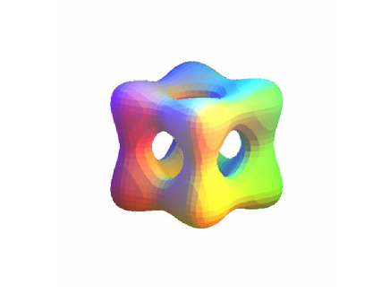
Figure 1: $F(x,y,z)=(x^{2}-1)^{2}+(y^{2}-1)^{2}+(z^{2}-1)^{2}-3/2$

6 Fourth application: Connectivity

There exist purely symbolic algorithms, based for instance on the notion of roadmap, to compute the connected components of $S$ (see Basu for further details. Here we propose an alternative approach to solve this question by means of a symbolic-numeric algorithm based on level curves. The empirical performance of this new method is quite satisfactory. The main idea of the algorithm is to determine how the connected components of a level curve corresponding to a non-critical $z$-value join to the connected components of the level curves corresponding to the critical level values immediately below and above, respectively. For this purpose, we take points on each connected component of the non-critical $z$-value, and then we generate a space curve (as the solution of a system of differential equations) which connects it with some connected component of the critical $z$-level curve immediately below/above (see Figure 2). Thus, once we know how to join the connected components of the level curves corresponding to non-critical and critical $z$-values, the number of connected components of $S$ can be obtained as the number of “connected chains” (whose elements are connected components of level curves) computed in the process.

In order to solve this problem, we require some more conditions on the surface $S$ to be analyzed. More precisely, the following hypotheses must be satisfied:

• $S$ is defined by an square-free polynomial $F$, with no factor just depending on the variables $y,z$. If this holds, then $\gcd(F,F_{x})=1$, so the variety ${\mathcal{C}}$ defined by $F=F_{x}=0$ is a space algebraic curve; recall that $F_{x}$ denotes the partial derivative of $F$ w.r.t. $x$.

• There does not exist any plane $z-a=0$ containing infinitely many points of the curve ${\mathcal{C}}$ introduced in (i), i.e. not containing infinitely many points of $S$ where $F_{x}$ vanishes.

• $S$ is not asymptotic to any plane of equation $z-b=0$, where $b$ is a critical level value.

Observe that in case that $S$ does not fulfill some of these conditions, almost all linear transformations lead to a new surface where the three requirements hold. Note that linear transformations preserve the topological features of the surface.

Now, in the sequel let ${\mathcal{A}}=\{a_{1},\ldots,a_{r}\}$, where $a_{1}<\cdots<a_{r}$, be a $z$-critical level set of $S$; furthermore, we set $a_{0}=-\infty$, $a_{r+1}=+\infty$. Moreover, let $b_{0}<\cdots<b_{r}$ verify $a_{i}<b_{i}<a_{i+1}$ for all $i\in\{0,\ldots,r\}$. With this notation, our problem is to decide, for each $a_{i},b_{i},a_{i+1}$, how to connect the connected components of the level curves $S_{b_{i}},S_{a_{i}}$, and $S_{b_{i}},S_{a_{i+1}}$, respectively. Observe that computing the topology graph of a level curve (which is planar) one obtains the connected components of it (see for instance Lalo ). Also, note that it may happen that the level curves for values in some of the intervals $(a_{i},b_{i})$ are empty over the reals, in which case there is no need of connecting $S_{b_{i}},S_{a_{i}}$, and $S_{b_{i}},S_{a_{i+1}}$. In addition, observe that, since $S$ verifies condition (iii), every connected component of some level curve of $S$ corresponding to a non-critical $z$-value, joins to some connected component of the level curve corresponding to the $z$-critical level value immediately below (resp. above). In fact, this is the reason why we request condition (iii).

For this purpose, the strategy is to use a symbolic-numeric algorithm which essentially works as follows:

Algorithm: (Connected components of an algebraic surface $S$) Given an algebraic surface $S$ implicitly defined by a real polynomial $F(x,y,z)$ verifying the conditions (i), (ii), (iii), the algorithm determines the number of connected components of $S$ and a description of them in terms of level curves.

• Compute the topology graph of $S_{b_{i}}$ (if $S_{b_{i}}\cap{\mathbb{R}}^{3}=\emptyset$ take another $i$), and the singular points of $S_{a_{i}}$; the information on the singular points of $S_{a_{i}}$ will be used at step (2), in some cases (see Remark 4), and also at step (3)).

• Take a real point $P$ in each connected component of $S_{b_{i}}$.

• Use a path continuation method to connect $P$ with some point $Q$ in $S_{a_{i}}$, to be computed by the algorithm; in order to do this, we travel from $P$ to $Q$ by following a space curve, contained in the surface, which is computed as the solution of a system of differential equations.

• Identify the connected component of $S_{a_{i}}$ where the final point $Q$ belongs to. For this purpose, we compute the topology graph of $S_{a_{i}}$ introducing the point $Q$ as a vertex of the graph.

• Join by an edge the starting connected component of $S_{b_{i}}$ and the finally reached connected component of $S_{a_{i}}$.

• Proceed in an analogous way to connect $P$ with some point $Q^{\star}$ in $S_{a_{i+1}}$.

• After carrying out the computation for all the connected components of all the $S_{b_{i}}$, one gets several connected chains, each one consisting of some connected components of the $S_{b_{i}}$, $S_{a_{i}}$ joined by edges. The number of connected chains, is the number of connected components of the surface.

Observe that in the execution of step (0), points on each connected component of $S_{b_{i}}$ are computed (see e.g. Lalo or Hong ), so step (1) can be executed afterwards. Now, let us describe with more detail step (2). We consider the solution to the following system of differential equations:

$$\left\{\begin{array}[]{l}x^{\prime}=-F_{y}+\displaystyle{\frac{F_{z}}{F_{x}}}\\ y^{\prime}=F_{x}\\ z^{\prime}=-1\\ x(0)=x_{i};y(0)=y_{i};z(0)=b_{i}\end{array}\right.$$

where $P:=(x_{i},y_{i},b_{i})\in S_{b_{i}}$. In case that this differential system has a symbolic solution $(x(t),y(t),z(t))$, one may see that it corresponds to a space curve contained in $S$. Moreover, since $z^{\prime}(t)=-1$ and $S$ fulfills condition (iii), then this space curve reaches $z=a_{i}$. Furthermore, since one may decompose the part of $S$ with $z\in(a_{i},b_{i})$ into non-intersecting pieces, each one corresponding to a different connected component of $S_{b_{i}}$ (see JGRS for a careful proof of this fact), the choice of the initial point for a particular connected component of $S_{b_{i}}$ does not affect the connected component finally reached. In other words, the connected component reached at $z=a_{i}$ is always the same for all the points of a same connected component of $S_{b_{i}}$ (see also Figure 2).

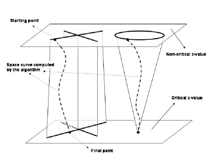
Figure 2: Idea of the connectivity algorithm

However, in general the differential system above may not have a symbolic solution, so numerical methods must be applied. In our case, we used the package of maple for numerically integrating differential equations. Here, one may see that as the numerical method goes on, the error considerably grows, so the point of $z=a_{i}$ finally reached cannot be recognized as belonging to any connected component of $S_{a_{i}}$. For this purpose, at each step the solution provided by numerical integration must be corrected. In order to do this, each solution $\tilde{P}_{i,k}=(\tilde{x}_{i,k},\tilde{y}_{i,k},\tilde{z}_{i,k})$ is corrected to $\bar{P}_{i,k}=(\bar{x}_{i,k},\bar{y}_{i,k},\tilde{z}_{i,k})$ by computing a point of the level curve $S_{\tilde{z}_{i,k}}$ close to the solution $(\tilde{x}_{i,k},\tilde{y}_{i,k},\tilde{z}_{i,k})$ (observe that the $z$-coordinate is the same in $\tilde{P}_{i,k}$ and in $\bar{P}_{i,k}$). For this purpose, we take the line passing through $\tilde{P}_{i,k}$ in the direction of $\vec{v}=(F_{x}(\tilde{P}_{i,k}),F_{y}(\tilde{P}_{i,k}))$, and we compute the intersection points of this line with $S_{\tilde{z}_{i,k}}$. This new point is used to go on with the numerical integration process. Although we have not analyzed the convergence of the method, the empirical results we get in this way are satisfactory. In this sense, the following remark must be taken into account.

Remark 4

If $K$ is a singular point of $S_{a_{i}}$ (notice that these points are computed in the initial step of the algorithm), then we assume that it is reached whenever the distance between $\bar{P}_{i,k}$ and $K$ is smaller than a sufficiently small $\epsilon$ previously fixed. Thus, in this case the computation stops and we assume that the starting point of $S_{b_{i}}$ is connected with $K$, i.e. that $Q=K$.

In addition, there are two more situations which must be examined carefully:

• If, before reaching the level plane $z=a_{i}$, the numerical integration process hits a point where $F_{x}$ vanishes, then the method fails. This situation can be prevented by detecting whether $|F_{x}(\tilde{x}_{i,k},\tilde{y}_{i,k},\tilde{z}_{i,k})|<\epsilon$; if this happens, we choose a different point of $S_{\tilde{z}_{i,k}}$ to go on with the numerical process.

• It may happen that $S$ contains a 1-dimensional subset ${\mathcal{L}}$ of singular points, where ${\mathcal{L}}$ is “isolated” in the following sense: given any point $P\in{\mathcal{L}}$, there exists a Euclidean neighborhood $E_{p}$ of $P$ such that every point of $S\cap E_{p}\cap{\mathbb{R}}^{3}$ is also a point of ${\mathcal{L}}$. For example, the handle of the Whitney Umbrella $x^{2}-y^{2}z=0$, which is obtained for negative values of $z$, provides an example of this situation. Unless ${\mathcal{L}}$ is parallel to the $xy$-plane, this phenomenon can be detected by identifying the presence of isolated points in non-critical level curves.

  Hence, assume that $S_{b_{i}}$ has some isolated point $B$, therefore belonging to some ${\mathcal{L}}$. The points of ${\mathcal{L}}$ are singular points of $S$, so $F_{x}$ vanishes at $B$ and therefore the system of differential equations before cannot be used to compute the point $A$ in $S_{a_{i}}$ which must be connected with $B$. Now, in this case we use the projections of the curve ${\mathcal{L}}$ onto two coordinates planes to compute how the points of ${\mathcal{L}}$ in $z=b_{i}$ and $z=a_{i}$, respectively, are connected, in analogy with the method described in JG-Sendra to compute the topology of space algebraic curves. More precisely, we consider a coordinate plane so ${\mathcal{L}}$ is not normal to it. We project ${\mathcal{L}}$ onto this plane, we determine the projection $\pi(B)$ of the point $B$, and then we determine the projection $\pi(A)$ of the point $A$ by either applying a path continuation method (over the projection), or by computing the part of the graph associated with the projection between $z=b_{i}$ and $z=a_{i}$. Carrying out this process on two coordinate planes, the point $A$ is obtained.

Finally, in order to connect $z=b_{i}$ and $z=a_{i+1}$, we apply an analogous process to the differential equation system:

$$\left\{\begin{array}[]{l}x^{\prime}=-F_{y}-\displaystyle{\frac{F_{z}}{F_{x}}}\\ y^{\prime}=F_{x}\\ z^{\prime}=1\\ x(0)=x_{i};y(0)=y_{i};z(0)=b_{i}\end{array}\right.$$

Note here that the third equation is different from the system before ($z^{\prime}=1$ instead of $z^{\prime}=-1$), since in this case one has to move “up” from $z=b_{i}$ to $z=a_{i+1}$. One may see that also the first equation has changed. However, the space curve that one obtains by integrating these equations lies also in the surface $S$.

Example 5

Consider the algebraic surface $S$ defined by $F(x,y,z)=x^{2}+y^{2}+z^{2}+2xyz-1$. A $z$-critical level set of $S$ is ${\mathcal{A}}_{z}=\{-1,1\}$. Because of the symmetry of the surface, we have that ${\mathcal{A}}_{x}={\mathcal{A}}_{y}={\mathcal{A}}_{z}$, so for example $[-2,2]\times[-2,2]\times[-2,2]$ is suitable for plotting $S$. A plotting of $S$ in this interval can be seen in Figure 3; this figure was computed with maple.

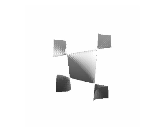
Figure 3: The cubic $x^{2}+y^{2}+z^{2}+2xyz-1=0$

Observe that, from Figure 3, it is not completely clear whether the surface is connected or not. However, using the algorithm we check that $S$ is connected. Indeed, Figure 4 shows the different topology types corresponding to the $z$-level curves for the cases $z<-1,z=-1,-1<z<1,z=1,z>1$, respectively. Moreover, also in Figure 4, each connected component of each $z$-level curve has been joined with the corresponding connected component of the $z$-critical level curve immediately above/below, according to the algorithm in this section. The connections between connected components of level curves are represented by dotted lines. Here, one may see that there is just one connected “chain”, formed by the connected components of the level curves which are joined one another. Hence, $S$ has just one connected component, and therefore it is connected.

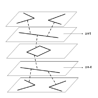
Figure 4: Connections between the level curves of $x^{2}+y^{2}+z^{2}+2xyz-1=0$

Example 6

Consider the quartic $(x^{2}-1)^{2}+(y^{2}-1)^{2}+(z^{2}-1)^{2}-3/4=0$. In this case, a $z$-critical level set of $S$ is

$${\mathcal{A}}_{z}=\{-1/2-\sqrt{3}/2,1/2-\sqrt{3}/2,-1/2+\sqrt{3}/2,1/2+\sqrt{3}/2\}$$

The different topology types for the $z$-level curves are shown in Figure 5; moreover, one may check that for $z>1/2+\sqrt{3}/2$ and $z<-1/2-\sqrt{3}/2$, the level curves are empty over ${\mathbb{R}}^{2}$. Furthermore, also in this picture we have represented (in dotted lines) how the connected components of these level curves are joined with each other. This information has been computed by using the algorithm in this section.

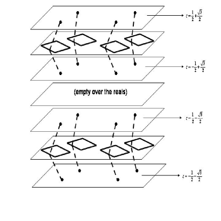
Figure 5: Connections between the level curves of $(x^{2}-1)^{2}+(y^{2}-1)^{2}+(z^{2}-1)^{2}-3/4=0$

Since in Figure 5 one may see 8 different connected chains of components of level curves, one has that $S$ has 8 connected components. A plotting of this quartic can be seen in Figure 6.

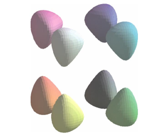
Figure 6: The quartic $(x^{2}-1)^{2}+(y^{2}-1)^{2}+(z^{2}-1)^{2}-3/4=0$

References

- (1) Alcazar J.G., Schicho J., Sendra R. (2007) A Delineability-based Method for Computing Critical Sets of Algebraic Surfaces, Journal of Symbolic Computation vol. 42, pp. 678-691.
- (2) Alcazar J.G., Sendra R. (2005) Computation of the Topology of Real Algebraic Space Curves, Journal of Symbolic Computation 39, pp. 719-744.
- (3) Alcazar J.G., Sendra R. (2007) Local Shape of Offsets to Algebraic Curves, Journal of Symbolic Computation vol. 42, pp. 338-351.
- (4) Basu S., Pollack R., Roy M.F. (2003) Algorithms in Real Algebraic Geometry , Springer Verlag.
- (5) Gonzalez-Vega L., Necula I. (2002). Efficient topology determination of implicitly defined algebraic plane curves, Computer aided geometric design, vol. 19 pp. 719-743.
- (6) Goresky M., MacPherson R. (1988). Stratified Morse Theory, Springer-Verlag.
- (7) Hong H. (1996). An effective method for analyzing the topology of plane real algebraic curves, Math. Comput. Simulation 42 pp. 571-582
- (8) Lang S. (1971). Algebra, Addison-Wesley.
- (9) MacCallum S. (1998). An Improved Projection Operation for Cylindrical Algebraic Decomposition. In Quantifier Elimination and Cylindrical Algebraic Decomposition (Eds. B.F. Caviness, J.R. Johnson), Spinger Verlag, pp.242–268.
- (10) Mignotte, M. (1992). Mathematics for Computer Algebra, Springer-Verlag.
- (11) Milnor, J. (1963). Morse Theory. Princeton University Press, Princeton N.J.
- (12) Mourrain B., Tecourt J. (2005). Isotopic Meshing of a Real Algebraic Surface, Rapport de recherche n 5508, Unite de Recherche INRIA Sophia Antipolis.
- (13) Sendra J., Sendra J. R. (2000). Algebraic Analysis of Offsets to Hypersurfaces. Mathematische Zeitschrift vol. 234, pp. 697–719.
- (14) Sendra J. R., Winkler F. (1999). Algorithms for Rational Real Algebraic Curves. Fundamenta Informaticae vol. 39, no. 1–2, pp. 211–228.
- (15) Winkler F. (1996), Polynomial Algorithms in Computer Algebra. Springer Verlag, ACM Press.