Complex Networks: Time–Dependent Connections and Silent Nodes

Abstract

We studied, both analytically and numerically, complex excitable networks, in which connections are time dependent and some of the nodes remain silent at each time step. More specifically, (a) there is a heterogenous distribution of connection weights and, depending on the current degree of order, some connections are reinforced/weakened with strength $\Phi$ on short–time scales, and (b) only a fraction $\rho$ of nodes are simultaneously active. The resulting dynamics has attractors which, for a range of $\Phi$ values and $\rho$ exceeding a threshold, become unstable, the instability depending critically on the value of $\rho.$ We observe that (i) the activity describes a trajectory in which the close neighborhood of some of the attractors is constantly visited, (ii) the number of attractors visited increases with $\rho,$ and (iii) the trajectory may change from regular to chaotic and vice versa as $\rho$ is, even slightly modified. Furthermore, (iv) time series show a power–law spectra under conditions in which the attractors’ space is most efficiently explored. We argue on the possible qualitative relevance of this phenomenology to networks in several natural contexts.

I Introduction and motivation

The concept of a network —defined as a sufficiently large set of nodes connected in pairs by edges— is potentially useful to help our understanding of the cooperative phenomena which are behind complex behavior in science and technology. Therefore, there has been a great interest for networks in physics during the last decade or so nets1 ; nets2 ; nets3 . Most of these studies have focused on the case in which the edge between any two nodes is either present or not. This relatively simple situation allows one to investigate, in particular, wiring topology which, for example, has lead to the discovery of scale–free and small–world networks in natural and man–made systems. However, real networks exhibit a number of relevant qualities besides interesting topological structure nets3 ; complex1 ; complex2 ; complex2a ; complex3 ; complex4 . In this paper, we are concerned with two features which could be essential to a network demeanor:

(a) Weighted and time–dependent connections. Very generally, intensities and/or capacities vary notably from one edge to the other in actual networks. For instance, a main feature of trophic webs is the complexity of pattern flows along the food chains, the agents in social and communication (e.g., cell phone) networks exchange assets or information according to various rules and depending on their partners, transport connections differ in capacity and actual number of transits and passengers, and effective ionic interactions constantly vary in condensed matter due to reactions as well as to diffusion and local rearrangements of ions and impurities. It is to be stressed that the connection weights in these cases often vary with time. There are variations of weights on a long–time scale. Their main purpose seems to be determining the nature and degree of heterogeneity the network needs for its intended function, say, computation, transport, cooperation, etc. In addition, although perhaps less investigated yet, weights may change on a short–time scale to improve actual functioning. To our knowledge, the best documented cases so far of such fast fluctuations do not belong to physics but to computational and neural networks. As a matter of fact, the human brain is the paradigm of a weighted network brainweight ; 9bis , and it is also clear–cut that high–level functions in the brain rely on fast synaptic changes during operation abb . Consequently, as we have a main interest here on short–time weight variations, we shall in the following often use the language and refer to observations on neural and, eventually, computational networks. In any case, our setting is rather general and we believe that the main behavior described in this paper should apply to networks in different contexts (see, for instance, Refs. complex2 ; complex3 ).

(b) Partial activation of nodes. In addition to the above —and perhaps also a further source of fast fluctuations—, one may argue that there is no need for a network to maintain all the nodes fully informed of the activity of all the others at all times. Relaxing such situation would both simplify the case and turn operation more economical. Moreover, there are some indications that certain nodes are more active than others, and that only a fraction of nodes is actually engaged at each time in some cooperative tasks. For example, this is the characteristic behavior of excitable media in which elements, after responding to perturbation, are refractory to further excitation exci ; julyan . This is interesting because such behavior could sometimes reveal to the observer as (relatively) fast time variations of connections as described above. The possibility of having reticent nodes is also a recent concern in computer science in relation with parallelism computer0 ; computer , in mathematical–physics phys , and in neuroscience, where it has been associated with working memories micro ; workmem ; wage , variability of neuron thresholds threshold and silent neurons silent ; silent2 . On the other hand, there is evidence of partial synchronization in many different situations sincro . In principle, this is a different phenomenon but one may argue that some of the observed partial synchronization processes, in which some elements do not attend to the others’ mode, could be associated with the existence of silent and/or excitable units, the case of interest here. In any case, studying the effect of updating only a fraction of nodes will certainly shed light on the possible consequences of having partial synchronization in the network.

The investigation of (a) in physics has only recently been initiated. As an example we mention the observed aging of nodes, e.g., in the networks of scientific publications where original papers stop receiving links after a finite time because review papers are then cited instead 22bis ; see also, for instance, Refs.complex1 ; complex2 ; complex2a ; complex3 ; complex4 . However, studying the consequences of fast connection changes in biologically inspired models has already a two–decades history —see cortesNC and references therein. For example, it has recently been shown that the susceptibility of a network to outside influence increases dramatically for excitable nodes mauro and, more specifically, under a competition of processes which tend to increase and decrease, respectively, the efficiency of synaptic connections at short times facilitation . To the best of our knowledge, investigation of feature (b) is rarer herzPRE ; phys ; computer ; LinksNodes , in spite of the fact that there is some —as mentioned above— specific motivation for it in several fields. Trying to understand the combined effect of these two features, (a) and (b), is a main objective here. We show that varying the fraction of nodes that are simultaneously active induces a variety of qualitatively different behaviors when the system is in a state of great susceptibility, but not in more general conditions. The susceptibility needed to observe the most interesting behavior is shown to occur under appropriate tuning of the connection weights with the network activity. It thus ensues that the effects of (a) and (b) are correlated with each other —which confirms a suspicion mentioned in the description of (b) above. Even more, it seems that the concurrence of (a) and (b) could be needed in some occasions in nature. As a first application, we describe here how a model exhibits unstable dynamics, which leads to itinerancy and chaotic behavior in a way that mimics both general expectations and some recent biological observations.

II Definition of a simple dynamic network model

A full description of the network configuration requires both the set of node states or activities, $s$$\equiv\left\{s_{i}\right\},$ and the set of connection weights, $\mathbf{w\equiv}\left\{w_{ij}\in\mathbb{R}\right\},$ where, $i,j=1,\ldots,N.$ From these we define a local field on each node due to the weighted action of the others, namely, $h_{i}\left(\mathbf{s},\mathbf{w}\right)\equiv\sum_{j\neq i}w_{ij}s_{j}.$ At each time unit, one updates the activity of $n$ nodes, with $1\leqslant n\leqslant N.$ This induces evolution in discrete time, $t,$ of the configuration probability distribution according to the master equation:

$$P_{t+1}(\mathbf{s})=\sum_{\mathbf{s}^{{}^{\prime}}}\text{{T}}\left(\mathbf{s}^{\prime}\mathbf{\rightarrow s}\right)P_{t}(\mathbf{s}^{\prime}),$$ (1)

where the transition probability may be written as

$$\text{{T}}\left(\mathbf{s\rightarrow s}^{\prime}\right)=\sum_{\mathbf{x}}p_{n}(\mathbf{x})\prod_{\left\{i|x_{i}=1\right\}}\tau_{n}\left(s_{i}\rightarrow s_{i}^{\prime}\right)\prod_{\left\{i|x_{i}=0\right\}}\delta_{s_{i},s_{i}^{\prime}}.$$ (2)

Here, $\mathbf{x}$ is an operational set of binary indexes —fixed to $1$ at $n$ sites chosen at each time according to distribution $p_{n}\left(\mathbf{x}\right),$ and fixed to zero at the other $N-n$ sites. The choice (2) simply states that one (only) updates simultaneously the selected $n$ nodes. The corresponding elementary rate is

$$\tau_{n}\left(s_{i}\rightarrow s_{i}^{\prime}\right)=\sigma\left(s_{i}\rightarrow s_{i}^{\prime}\right)\left[1+\left(\delta_{s_{i}^{\prime},-s_{i}}-1\right)\delta_{n,1}\right],$$ (3)

where $\sigma=\sigma\left(\mathbf{s},\beta\right)$ is a function to be determined, with $\beta$ an inverse temperature parameter.

The above describes parallel updating, as in cellular automata, for $n=N$ or, macroscopically, $\rho\equiv n/N\rightarrow 1.$ However, the model describes sequential updating, as in kinetic magnetic models, for $n=1$ or $\rho\rightarrow 0.$ We are interested in changes with $\rho\in\left(0,1\right).$ In addition to allow for a sensible generalization of familiar cellular automata, this bears some practical interest, as indicated in the introduction. For example, assuming a neural network, $\rho$ may stand for the fraction of neurons that are stimulated each cycle. There is no input on the other $1-\rho,$ so that information from the previous state is maintained. This induces persistent activity which has been argued to be a basis for working memory micro ; workmem ; wage . Varying $\rho$ may also be relevant to simulate the observed variability of the neurons’ threshold threshold and the possible existence of silent neurons silent or dark neuro–matter silent2 , for instance. These are just examples of the fact that varying $\rho$ has a great general interest to better understanding excitable media.

The equations above may be simulated in a computer for different choices of $p_{n}$ and transition details. In order to obtain analytical results, however, we need to simplify the model somewhat. That is, we shall refer to the case in which the node activities are binary, $s_{i}=\pm 1,$ the $n$ nodes to be updated are chosen at random, so that one has $p_{n}\left(\mathbf{x}\right)=\tbinom{N}{n}^{-1}\delta\left(\sum_{i}x_{i}-n\right),$ and $\sigma$ in (3) is an arbitrary function of (only) $\beta s_{i}h_{i}$ which satisfies detailed balance. In spite of the latter, detailed balance is not fulfilled by the superposition T for $n>1,$ so that resulting steady states are generally out of equilibrium, which is known to be realistic marroB . On the other hand, for simplicity, in order to be able to obtain some analytical results, we shall assume that the fields are such that $h_{i}\left(\mathbf{s},\mathbf{w}\right)=h\left[\mathbf{\pi}\left(\mathbf{s}\right),\mathbf{\xi}_{i}\right].$ Here, $\mathbf{\xi}_{i}\equiv\left\{\xi_{i}^{\mu}=\pm 1;\mu=1,\ldots,M\right\}$ stands for $M$ given realizations of the set of activities, or patterns, and $\mathbf{\pi}\equiv\left\{\pi^{\mu}\left(\mathbf{s}\right)\right\},$ where

$$\pi^{\mu}\left(\mathbf{s}\right)=N^{-1}\sum_{i}\xi_{i}^{\mu}s_{i},$$ (4)

measures the overlap between the current state and pattern $\mu.$ For $N\rightarrow\infty$ and finite $M,$ i.e., in the limit $\alpha\equiv M/N\rightarrow 0,$ the time equation

$$\pi_{t+1}^{\mu}\left(\mathbf{s}\right)=\rho N^{-1}\sum\nolimits_{i}\xi_{i}^{\mu}\tanh\left\{\beta h_{i}\left[\mathbf{\pi}_{t}\left(\mathbf{s}\right),\mathbf{\xi}_{i}\right]\right\}+\left(1-\rho\right)\pi_{t}^{\mu}\left(\mathbf{s}\right)$$ (5)

follows for any $\mu.$ Actual applications concern finite values for both $M$ and $N,$ so that the limit $\alpha\rightarrow 0$ is not very intesreting in practice. This and other restrictions are not essential to the model, however; in fact, our simulations below concern more general situations, as pointed out when necessary.

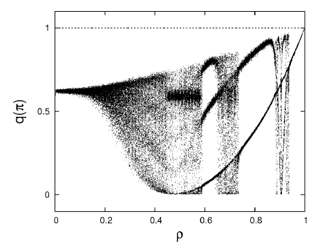
Figure 1: Evidence of chaos. Bifurcation diagram showing the stationary order parameter $q\left(\mathbf{\pi}\right),$ as defined in the main text, versus the synchronization parameter $\rho$ for $M=20$ random patterns, $N=3600$ nodes, $\beta=20$ and $\Phi=-1/2.$ This behavior is characteristic of any $\Phi\neq 1,$ and it follows indistinctly from the analytical solution and from Monte Carlo simulations.

The model allows for different relations between the fields $h_{i}$ and the other network properties. The simplest case at hand for specific relations of such kind is Hopfield’s hopf1 which follows here for $\rho\rightarrow 0$ and weights fixed according to the Hebb prescription, i.e., $w_{ij}=N^{-1}\sum_{\mu}\xi_{i}^{\mu}\xi_{j}^{\mu}.$ The symmetry $w_{ij}=w_{ji}$ then assures $P_{t\rightarrow\infty}\left(\mathbf{s}\right)\propto\exp\left(\beta\sum_{i}h_{i}s_{i}\right).$ This corresponds to thermodynamic equilibrium and —using the neural–network argot— this is a case that exhibits associative memory. This means that, for high enough $\beta,$ the patterns $\left\{\mathbf{\xi}_{i}\right\}$ are attractors of dynamics hopf2 , as if they would have been stored in the connections and recalled in the course of the system relaxation with time. Equilibrium is generally impeded for $\rho>0$ grin , and the asymptotic state then strongly depends on dynamic details marroB ; odorRMP . We checked that, in agreement with some indications herzPRE , the Hopfield–Hebb network also exhibits associative memory for $\rho>0.$ However, no new physics emerges as $\rho$ is varied in this case, and it is likely this occurs rather generally concerning dynamics for simple weighted networks.

Figure 2: Lyapunov surface. The Lyapunov exponent as a function of $\beta$ for $\Phi=0.01$ (top), and as a function of $\Phi$ for $\beta=25$ (bottom), as obtained from the saddle–point map (5). The black regions and curves correspond to a positive Lyapunov exponent, so that dynamics is then irrregular. The white regions correspond to a negative Lyapunov exponent associated with regular behavior. Note a small black, chaotic region for $\rho\lesssim 1$ and low $\beta$ in the upper graph.

Our model may exhibit a complex dependence on $\rho$ assuming activity dependent weights. This is expected to occur in many cases, e.g., for excitable media exci ; julyan . However, as far as we know, the only situation with time–dependent connections which is well documented in the literature concerns the brain. In this case, transmission of information and computations have repeatedly been reported to be correlated with activity–induced fast fluctuations of synapses, i.e., our $w_{ij}$’s noise ; abb . For example, it has been observed that the efficacy of synaptic transmission can undergo short–time increasing (sometimes called facilitation) facil ; facil2 ; Wang or decreasing (depression) depre000 ; 9 ; abb0 , and that these effects depend on the activity of the presynaptic neuron. Furthermore, it has already been demonstrated that such processes may importantly affect a network performance cortesNC ; facilitation ; depre1 ; bibit ; Romani . Likewise, it seems sensible to assume that similar short–time variations may occur in other networks —e.g., reaction–diffusion systems and the cardiac tissue julyan — associated with some efficacy lost after heavy work or with excitations, for instance.

Motivated by all these facts, and also trying to maintain a well–defined reference frame, we shall assume that the connection weights are

$$w_{ij}=\varepsilon_{ij}\overline{w}_{ij}=\varepsilon_{j}\overline{w}_{ij},$$ (6)

where the second equality is introduced for simplicity. Here, $\overline{w}_{ij}$ stands for some reference value and $\varepsilon_{j}$ for a random variable. That is, we are assuming some “noise” on top of a previous preparation of the connections designed so that the network can perform some specific function. The background just described also suggests us to assume that the random variable in (6) is fluctuating very rapidly so that, on the time scale for the activity changes, it behaves as stationary with distribution given, for example, by

$$p^{\text{st}}\left(\mathbf{s},\varepsilon_{j}\right)=q\delta\left(\varepsilon_{j}-\Phi\right)+\left(1-q\right)\delta\left(\varepsilon_{j}-1\right).$$ (7)

We shall further assume that $q$ depends on the degree of order in the system at time $t,$ namely, that $q=q\left(\mathbf{\pi}_{t}\right).$ For the sake of concreteness, our choices here will be that $q\left(\mathbf{\pi}\right)=\left(1+\alpha\right)^{-1}\sum_{\mu}\pi^{\mu}\left(\mathbf{s}\right)^{2}$ and that $\overline{w}_{ij}$ is given by the Hebb prescription. The result is that each node is acted on by an effective field

$$h_{i}^{\text{eff}}\left(\mathbf{s},\mathbf{w}\right)=\sum_{j\neq i}w_{ij}^{\text{eff}}s_{j}$$ (8)

with $w_{ij}^{\text{eff}}=\left[1-\left(1-\Phi\right)q\left(\mathbf{\pi}\right)\right]\overline{w}_{ij}.$ This amounts, in summary, to assume short–term variations which change the intensity or capacity of connections by an amount, either positive or negative, $\Phi$ on the average. More specifically, one has a decreasing effect for any $\Phi<1$, and enhancement for $\Phi>1,$ as far as $\Phi>0,$ while $\Phi<0$ induces a change of sign. For the indicated choices of fields and reference weights, our framework reduces to the familiar Hopfield–Hebb case for $\Phi=1.$ Note that it should not be difficult to implement the model for choices other than (6) and (7).

III Description of main results

Assuming (8), it readily ensues from (5) for $M=1$ that $\pi_{\infty}=F\left(\pi_{\infty};\rho,\Phi\right)$ and that local stability requires that $\left|\partial F/\partial\pi\right|<1,$ where

$$F\left(\pi;\rho,\Phi\right)\equiv\rho\tanh\left\{\beta\pi\left[1-\left(1-\Phi\right)\pi^{2}\right]\right\}+\left(1-\rho\right)\pi.$$ (9)

Therefore, fixed points are independent of $\rho$ for any $\Phi,$ but stability demands that $\rho<\rho_{c}$ with $\rho_{c}=2\left\{3\beta\pi_{\infty}^{2}\left[\left({\frac{4}{3}-}\Phi\right)-\left(1-\Phi\right)\pi_{\infty}^{2}\right]-\beta+1\right\}^{-1}.$ The resulting situation for any $\Phi\neq 1$ is illustrated in Fig. 1, where one observes regular behavior, bifurcations and chaotic windows. This picture cannot occur for fixed weights, e.g., in the Hopfield case. In order to deepen on the possibility of chaos, we computed the Lyapunov surface from the analytical solution for $M=1.$ Two sections of this surface are shown in Fig. 2. This clearly reveals the existence of chaos above some degree of synchronization, namely, for $\rho\geq\rho_{\ast}\left(\beta,\Phi\right)>\rho_{c}\left(\beta,\Phi\right)$ where the latter marks the onset of period doubling before irregular behavior. For example, the top graph shows that, for a small positive value of $\Phi,$ which corresponds to some slight depression of connections which occurs more likely the higher the current system order is, there is a region for large $\beta$ (relatively small temperature, say $T\approx 0.02$ in our arbitrary units) and $1>\rho\gtrsim 0.8$ for which dynamics may eventually become chaotic. In the same graph one may notice a tiny chaotic window for $\rho\approx 1$ and $\beta\approx 7;$ this is the case identified previously by us chaos . The bottom graph, on the other hand, illustrates that chaos is typically an exception for positive values of $\Phi;$ it may only occur then for a rather large fraction of synchronized nodes (large $\rho)$ near $\Phi\lesssim 0.$ On the contrary, for negative $\Phi,$ i.e., when the order tends to induce changes of sign of the connection intensities, it is more likely that the system will behave chaotically. It is also to be remarked that, inside the first, more exterior curve in each graph, there is a complex pattern of transitions from regular to irregular behavior as one changes, even very slightly the values of $\rho,$ $\Phi$ and $\beta.$ As one may imagine, this situation for very small $M$ gets even more involved as $M$ increases. Finally, it is noticeable the fact that chaotic switching among different patterns was recently demonstrated to occur also in the thermodynamic limit LT . The next question is whether such complex behavior may have some constructive role in natural and man–made networks.

Figure 3: Typical Monte Carlo runs. This shows the overlap as a function of time (in units of $n$ MC trials), during the stationary regime after equilibration, for $N=1600$ nodes, $\beta=50,$ $\Phi=0.004$ and, from bottom to top, $\rho=0,$ 0.60, 0.87, 0.93 and 1.00, respectively. In this case, the onset of period doubling before irregular behavior is at $\rho=\rho_{c}\simeq 0.5.$ This is for $M=3$ correlated patterns (identified here with different colours). That is, we generated three patterns completely at random, and then replaced 20% of the digits in the second and third patterns with the same number of digits, and flipped digits, respectively, taken from the first pattern.

Different types of behavior the system may exhibit are illustrated by the stationary Monte Carlo runs in Fig. 3. This involves three partially correlated patterns, as explained in the figure caption, and illustrates, from bottom to top:

1. For $\rho<\rho_{\ast},$ convergence towards one of the attractors, namely, fixed points corresponding to the patterns provided. This is revealed by the fact that one of the overlaps (the red one in this case) is constantly rather large, close to 1, while the others two are closer to zero (they differ from zero due to the built correlations between patterns).

2. Irregular behavior with positive Lyapunov exponent for a larger value of $\rho.$ Notice that changes with time indicate that dynamics is now unstable and the system activity is visiting the different attractors, including the negative of some of them or antipatterns.

3. A different type of irregular behavior in which, in addition to visiting different attractors on a large time scale, there are much more rapid irregular transitions between one pattern and its antipattern.

4. Regular oscillation between one attractor and its negative.

5. Rapid and ordered periodic oscillations between one pattern and its antipattern when all the nodes are active.

The cases 2 and 3 are examples of instability–induced switching phenomena, namely, the system describes heteroclinic paths among the attractors, and remains different time intervals in the neighborhood of each of them, as it was previously observed in a related case chaos .

Figure 4: Monte Carlo runs that one may interpret as states of attention in the network, which illustrates the possible role of chaos. This shows phase–space trajectories of the mean firing rate for $N=1600,$ $\beta=167,$ $\Phi=-{\frac{1}{2}},$ and, from left to right, $\rho=$ 0.384, 0.39 and 0.4. Here, $\rho_{c}=0.38,$ and the system stores three patterns, $\xi^{\mu},$ $\mu=1,2$ and 3, as described in the main text. (These graphs involve a standard false–neighbor method embed with embedding dimension $d_{e}=5$ and time delay $\tau=5.)$

An interesting fact concerning the nature of the phase space trajectory as $\rho$ is varied is illustrated in Fig. 4. This shows time evolution of the mean firing rate defined as

$$m=\frac{1}{2N}\sum_{i=1}^{N}\left(1+s_{i}\right).$$ (10)

Three patterns (and their corresponding antipatterns) are involved here which consist of a string of 1s, a string with the first 50% positions set to 1 and the rest to $-1,$ and a string with only the first 20% positions set to 1, respectively. In the course of this Monte Carlo experiment, we observed that the activity remains wandering around one of the patterns for any $\rho<\rho_{\ast}$. The choice of pattern depends on the initial condition. For larger values of $\rho$ within a chaotic window, as for the three cases shown in Fig. 4, the system tends to visit the other patterns as well. In particular, the left–most case in the figure ($\rho=0.384)$ shows visits to the three patterns, and a trajectory which is structured, namely, there are many jumps between the pairs of more correlated patterns, and only a few between the most distant ones. Moreover, the number of jumps between the less correlated patterns tends to increase as $\rho$ is further increased within the chaotic window. The figure shows that, for $\rho=0.39$ and 0.40, even the antipatterns are visited; note that we have that $\mathbf{\xi}^{2}=-\mathbf{\xi}^{2}$. Increasing $\rho$ further, e.g., for $\rho=0.6$ in this specific experiment, the network surpasses equiprobability of patterns and, eventually, abandons the chaotic regime to fall into a limit cycle, where it periodically oscillates between a pattern and its antipattern.

Figure 5: Time series for the overlap $\pi$ in the case $\rho=0.632,$ $M=1,$ $\beta=\infty$ (zero temperature), $N=3600,$ and $\Phi=$ –0.048 (top) and –0.065 (bottom) showing chaotic transitions between the associated pattern and its antipattern. This series correspond to entropies $S\simeq$ 0.37 and 0.9, respectively.

In order to deepen further on the nature of the chaotic switching, we have computed the normalized power spectra $p\left(\omega\right)$ of the time series for the mean firing rate $m.$ If one computes the associated entropy bio , namely, $S=-\sum_{\omega}p_{\omega}\log$.$p_{\omega},$ it ensues a sharp minimum at $S\simeq 0.37$ for $\Phi=-0.048.$

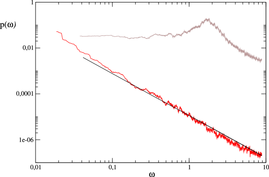
Figure 6: The power spectra corresponding to the two series in figure 5, i.e., for $\Phi=-0.065$ and $-0.048,$ respectively, for the upper and lower sets of data. The stright line here has negative slope 1.9.

The series corresponding to this minimum and, for comparison purposses, a different one for a much larger entropy are presented in figure 5. The power spectra for these two series is presented in figure 6. This reveals a qualitative change of behavior, namely, that (only) the series describing a more efficient chaotic mechanism exhibit a power law distribution. We are presently analyzing in more detail this interesting phenomenon. However, we can already illustrate further the situation as in figure 7.

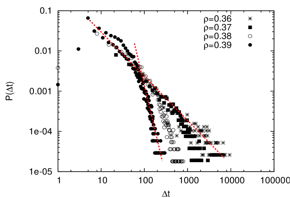
Figure 7: Distribution of the time intervals the network activity stays near each pattern during the computer experiment described in figura 4.

This shows the distribution for the time intervals the network activity spends wandering in the neighborhood of a particular attractor.

IV Discussion

We have described in this paper details concerning a model network in which connections are heterogeneously weighted and time–dependent, namely, correlated to the global activity. As documented above, these two conditions occur in many natural networks. Furthermore, only a fraction $\rho$ of nodes are active at each time, so that the rest maintain the previous state. This occurs in excitable media, for instance.

A main conclusion is that, although the synchronization parameter $\rho$ is generally irrelevant, varying $\rho$ may greatly modify the system behavior under certain conditions. The necessary condition is a kind of susceptibility or sensitivity to external stimuli which greatly favours dynamic instabilities. It may be achieved in our example by appropriate tuning of two parameters, $\Phi$ and $\beta.$ The latter is an inverse temperature which controls the stochasticity of the process. The former induces either enhancement ($\Phi>1)$ or lowering ($\Phi<1)$ for positive $\Phi,$ or even change of sign for negative $\Phi$, of the intensities of connections. This process is a very fast one —as compared with the nodes changes—, and it occurs more likely the larger the current degree of order is. The interesting behavior described in this paper washes out if the connection weights are fixed, even heterogeneously as, for instance, in a Hopfield–Hebb network, which corresponds here to $\Phi=1.$

Within the most interesting range for its parameters, our model exhibits heteroclinic trajectories which imply, in particular, a kind of dynamic association. That is, the network activity either goes to one attractor for $\rho<\rho_{\ast},$ or else, for larger $\rho,$ is capable of an intriguing programme of visits to possible attractors. The dynamic path followed during these visits may abruptly become chaotic, which seems the most relevant regime. Besides synchronization of a minimum of nodes, this requires careful tuning of $\rho,$ $\beta$ and $\Phi.$ That is, as suggested by Fig. 2, there is a complex parameter space which makes it difficult to predict the ensuing behavior for slight changes of parameter values. Note in this respect that figure 2 is for $M=3$ patterns only, and that the corresponding picture greatly complicates as $M$ is increased.

The most interesting behavior of the network consists of switching among attractors. We observe regular switching in some occasions for $\rho<\rho_{\ast},$ but chaos makes such process much more efficient. Therefore, our model confirms expectations caos1 ; caos2 ; attent3 that the instability inherent to chaos facilitates moving to any pattern at any time, and that chaos and chaotic itinerancy may be the strategy of nature to solve some difficult problems caos10 ; caos11 . Consistent with this, we have illustrated above a specific mechanism which allows for an efficient search of the attractors’ space. More specifically, we observe a highly–structured chaotic itinerancy process in which, as illustrated in Fig. 4, modifying $\rho$ within a chaotic window —which requires also tuning $\beta$ and $\Phi$— one may control the subset of visited attractors. That is, increasing $\rho$ within the relevant regime makes the system to visit more distant (less correlated) attractors. In this way the system may perform, for instance, family discrimination and classification by tuning $\rho$ algo . On the other hand, the complexity of the parameter space for $\rho>\rho_{\ast}$ suggest that one could devise a method to control chaos in these cases. It is also suggested that one should pay attention to these facts when determining efficient computational strategies in artificial machines. Similar switching phenomena, in which the activity describes a heteroclinic path among saddle states, has already been incorporated in models which thus simulate experiments on animal olfactory systems Rabi ; mazor ; huerta ; huerta2 ; attent3 ; olfato . Comparable oscillatory activity has been reported to occur in cultured neural networks wage and ecology models and food webs hof ; van ; van2 . This also seems to explain transitions between atmospheric patterns crom ; stew , and it is believed it could account for other natural phenomena as well attent3 .

Finally, an important feature of the model chaotic itinerancy is illustrated in figures 7 and 6. This reveals the existence of power–law distributions within the regimes in which the network exhibits its most interesting behavior. This is the case for the power spectra of time series and for the time spent in the neighborhood of each attractor for appropriate values of $\rho.$ This fact suggests that a critical condition which has been called for to explain some of the brain exceptional behavior crit1 ; crit2 ; crit3 ; crit4 ; chialvo could perhaps consists of a highly susceptible, unstable and chaotic condition similar to the one we have described for the model. The ocurrence of power–law behavior here is consistent with the approaching to zero of associated Lyapunov exponents, sometimes referred to as edge of chaos.

We acknowledge very useful discussions with S. de Franciscis, and financial support from FEDER–MEC project FIS2005-00791, JA project P06–FQM–01505, and EPSRC–COLAMN project EP/CO 10841/1.

References

- (1) A.L. Barabási, Rev. Mod. Phys. 74, 47 (2002)
- (2) M.E.J. Newman, SIAM Reviews 45, 167 (2003)
- (3) S. Boccaletti, V. Latora, Y. Moreno, M. Chavez, and D.U. Hwang, Phys. Rep. 424, 175 (2006)
- (4) M.E.J. Newman, Phys. Rev. E 70, 056131 (2004)
- (5) A. Barrat, M. Barthélemy, and A. Vespignani, Phys. Rev. E 70, 066149 (2004); ibid , J. Stat. Mech. P05003 (2005)
- (6) T. Antal and P.L. Krapivsky, Phys. rev. E 71, 026103 (2005)
- (7) M.A. Serrano, M. Boguñá, and R. Pastor–Satorras, Phys. Rev. E 74, 055101R (2006)
- (8) C. Zhou, A.E. Motter, and J. Kurths, Phys. Rev. Lett. 96, 034101 (2006)
- (9) R. Salvador, J. Suckling, M.R. Coleman, J.D. Pickard, D. Menon, and E. Bullmore, Cereb. Cortex 15,1332 (2005)
- (10) V.M. Eguíluz, D.R. Chialvo, G.A. Cecchi, M. Baliki, and A.V. Apkarian, Phys. Rev. Lett. 94, 018102 (2005)
- (11) L.F. Abbott and W.G. Regehr, Nature 431, 796 (2004)
- (12) E. Meron, Phys. Rep. 218, 1 (1992)
- (13) J.H.E. Cartwright, Phys. Rev. E 62, 1149 (2000)
- (14) G. Korniss, M.A. Novotny, H. Guclu, Z. Toroczkai, and P.A. Rikvold, Science 299, 677 (2003)
- (15) P. Tosic and G. Agha, in Proceedings of the First European Conference on Complex Systems ECCS’05, European Complex Systems Society, Paris, November 14-18 2005.
- (16) M.R. Evans, J. Phys. A: Math. Gen. 30, 5669 (1997)
- (17) A.V. Egorov, B.N. Hamam, E. Fransen, M.E. Hasselmo and A.A. Alonso, Nature 420, 173 (2000)
- (18) F.E. LeBeau, A. El Manira, and S. Griller, Trends Neurosci. 28, 552 (2005)
- (19) D.A. Wagenaar, Z. Nadasdy, and S.M. Potter, Phys. Rev. E 73, 051907 (2006)
- (20) R. Azouz and C.M. Gray, Proc. Natl. Acad. Sci. USA 97, 8110 (2000)
- (21) B.A. Olshausen and D.J. Field, Curr. Opin. Neurobiol. 14, 481 (2004)
- (22) S. Shoham, D.H. O’Connor, and R. Segev, J. Compar. Physiol. A 192, 777 (2006)
- (23) A. Pikovsky, M. Rosenblum, and J. Kurths, “Synchronization: A Universal Concept in Nonlinear Science”, Cambridge University Press, Cambridge 2001.
- (24) K. Klemm and V.M. Eguíluz, Phys. Rev. E 65, 036123 (2002)
- (25) J.M. Cortes, J.J. Torres, J. Marro, P.L. Garrido, and H.J. Kappen , Neural Comp. 18, 614 (2006)
- (26) O. Kinouchi and M. Copelli, Nat. Phys. 2, 348 (2006)
- (27) J.J. Torres, J. M. Cortes, J. Marro, and H.J. Kappen, Neurocomputing 70, 2022 (2007); ibid, Neural Comp. 19, 2739 (2007)
- (28) A.V.M. Herz and C.M. Marcus, Phys. Rev. E 47, 2155 (1993)
- (29) K. Park, Y. Lai, and N. Ye, Phys. Rev. E 70, 026109 (2004)
- (30) J. Marro and R. Dickman, “Nonequilibrium Phase Transitions in Lattice Models”, Cambridge Univ. Press, Cambridge 1999.
- (31) J.J. Hopfield, PNAS 79, 2554 (1982)
- (32) D.J. Amit, “Modeling Brain Function: Attractor Neural Networks”, Cambridge Univ. Press, Cambridge 1989.
- (33) G. Grinstein, C. Jayaprakash, and Y. He, Phys. Rev. Lett. 55, 2527 (1985)
- (34) G. Ódor, Rev. Mod. Phys. 76, 663 (2004)
- (35) D. Ferster, Science 273, 1812 (1996)
- (36) B. Katz and R. Miledi, J Physiol. 195, 481 (1968)
- (37) A. Reyes, R. Luján, A. Rozov, N. Burnashev, P. Somogyi, and B. Sakmann, Nat. Neurosci. 1, 279 (1998)
- (38) Y. Wang, H. Markram, P.H. Goodman, T.K. Berger, J. Ma, and P.S. Goldman-Rakic, Nat. Neurosci. 9, 534 (2006)
- (39) A.M. Thomson and J. Deuchars, Trend. Neurosci. 17, 119 (1994)
- (40) A.M. Thomson, J. Physiol. (London) 502, 131 (1997)
- (41) L.F. Abbott, J.A. Varela, K. Sen, and S.B. Nelson, Science 275, 220 (1997)
- (42) D. Bibitchkov, J. M. Herrmann, and T. Geisel, Network: Comp. Neural Syst. 13, 115 (2002)
- (43) L. Pantic, J.J. Torres, H.J. Kappen, and S.C.A.M. Gielen, Neural Comp. 14, 2903 (2002)
- (44) S. Romani, D.J. Amit, and G. Mongillo, J. Comp. Neurosci. 20, 201 (2006)
- (45) J. Marro, J.J. Torres, and J.M. Cortés, Neural Net. 20, 230 (2007)
- (46) J.J. Torres, J. Marro, and S. de Franciscis, preprint for Int. J. Bifur. Chaos (2008)
- (47) J.P. Eckmann and D. Ruelle, Rev. Mod. Phys. 57, 617 (1985)
- (48) J.M. Cortés, J.J. Torres, and J. Marro, Biosystems 87, 186 (2007)
- (49) H. Korn and P. Faure, C. R. Biologies 326, 787 (2003)
- (50) L. Glass, in “Handbook of Brain Theory and Neural Networks”, M.A. Arbib Ed., pp. 205, MIT Press, 2003.
- (51) P. Ashwin and M. Timme, Nature 436, 36 (2005)
- (52) L.F. Abbott and S.B. Nelson, Nature Neuroscience Supplement 3, 1178 (2000)
- (53) W.F. Freeman, Neurodynamics, Springer, London 2000.
- (54) J.M. Cortés et al., “Algorithms for identification and categorization”, AIP Conf. Proceed. 779, 178 (2005)
- (55) M. Rabinovich, A. Volkovskii, P. Lecanda, R. Huerta, H. Abarbanel, and G. Laurent, Phys. Rev. Lett. 87, 68102 (2001)
- (56) O. Mazor and G. Laurent, Neuron 48, 661 (2005)
- (57) R. Huerta, T. Nowotny, M. Garcia-Sanchez, H.D.I. Abarbanel, and M. I. Rabinovich, Neural Comput. 16, 1601 (2004)
- (58) R. Huerta and M. Rabinovich, Phys. Rev. Lett. 93, 238104 (2004)
- (59) J.J. Torres, J. Marro, J.M. Cortes, and B. Wemmenhove, submitted to Neural Net.
- (60) J. Hofbauer and K. Sigmund, J. Math. Biol. 27, 537 (1989)
- (61) J. Vandermeer, The Am. Naruralist 163, 857 (2004)
- (62) J. Vandermeer, H. Liere, and B. Lin, Theor. Popul. Biol., in press (2007)
- (63) D.T. Crommelin, J. Atm. Sci. 60, 229 (2003)
- (64) I. Steward, Nature 422, 571 (2003)
- (65) C.W. Eurich, J.M. Herrmann, and U.A. Ernst, Phys. Rev. E 66, 066137 (2002)
- (66) J.M. Beggs and D. Plenz, J. Neurosci. 23, 11167 (2003)
- (67) S. Bornholdt and T. Röhl, Phys. Rev. E 67, 066118 (2003)
- (68) C. Haldeman and J.M. Beggs, Phys. Rev. Lett. 94, 058101 (2005)
- (69) D.R. Chialvo, Nature Phys. 2, 301 (2006)